Multi-UAV Conflict Resolution with Graph Convolutional Reinforcement Learning

Abstract

Safety is the primary concern when it comes to air traffic. In-flight safety between Unmanned Aircraft Vehicles (UAVs) is ensured through pairwise separation minima, utilizing conflict detection and resolution methods. Existing methods mainly deal with pairwise conflicts, however, due to an expected increase in traffic density, encounters with more than two UAVs are likely to happen. In this paper, we model multi-UAV conflict resolution as a multiagent reinforcement learning problem. We implement an algorithm based on graph neural networks where cooperative agents can communicate to jointly generate resolution maneuvers. The model is evaluated in scenarios with 3 and 4 present agents. Results show that agents are able to successfully solve the multi-UAV conflicts through a cooperative strategy.

1. Introduction

Commercial and civil unmanned aircraft systems (UAS) applications are projected to have significant growth in the global market. According to SESAR, the European drone market will exceed 10 billion annually by 2035, and over 15 billion annually by 2050 [1]. Furthermore, considering the characteristics of the missions and application fields, it is expected that most market value will be in operations of small UAS (sUAS) and at the very-low-level airspace (VLL). Such a growing trend will be accompanied by an increase in traffic density and new challenges related to safety, reliability, and efficiency. Therefore, the development and implementation of conflict management systems are considered preconditions of integrating UAS in the civil airspace. Most notably, the National Aeronautics and Space Administration (NASA) in the USA aims to create a UAS Traffic Management (UTM) system that will make it possible for many UAS to fly at low altitudes along with other airspace users [2]. Europe is leading efforts to develop an equivalent UTM concept, referred to as U-space. It will provide a set of services (and micro-services) that would accommodate current and future traffic (mainly but not limited to) at VLL airspace [3]. Similar approaches are followed also in China and Japan [4]. Considering airspace under UTM services, UAS must be capable of avoiding static conflicts such as buildings, terrain, and no-fly zones and dynamic conflicts such as manned or unmanned aircraft. Here, a pairwise conflict is defined as a violation of the en-route separation minima between two UAVs [5]. To ensure operations free of conflict, UTM provides Conflict Detection and Resolution services, which comprise three layers of safety depending on the time-horizon (i.e., look-ahead time) [6]: Strategic and Tactical Conflict Mitigation and Collision Avoidance (CA) [5,6]. In this work, we will focus on tactical CR applicable for small UAS missions. This function is typically treated in two ways: self-separation and Collision Avoidance [6,7]. The former is a maneuver executed seconds before the loss of separation minima, characterized by a slight deviation from the initial flight plan, and aims to prevent CA activation. The latter provides a last-resort safety layer characterized by imminent and sharp escape maneuvers. Both functions above are encompassed within what is widely recognized as Detect and Avoid capability [8,9]. Aligning with the up-to-date state-of-the-art, a loss of separation minima is referred to as Loss of Well Clear (LoWC). While there is no standard definition of Well Clear (WC), two related functions are associated with this state: Remain Well Clear (RWC), and Collision Avoidance (CA) [10]. In terms of tactical CD&R, RWC is equivalent to the self-separation function. Defining and computing RWC thresholds are an open research works, but they are mainly viewed as protection volume around UAS [11,12,13]. This volume can be specified by spatial thresholds, temporal thresholds, or both at the same time. We follow the hockey-puck model [14,15] characterized by distance-based thresholds. In addition, the near-mid-air-collision (NMAC) represents the last safety volume. As the name suggests, a distance smaller than NMAC represents a very severe loss of well clear that could result in a collision in the worst case. This distance is usually defined based on the dimensions of the UAS and its navigation performance [16].

There are many existing works that propose conflict resolution algorithms (see Section 2 for a more detailed overview). However, the majority of these works focus mainly on pairwise conflicts. Nevertheless, with the expected increase in traffic density [1] multi-UAV conflicts (i.e., involving more than 2 UAVs) are expected to occur. In this paper, multi-UAV conflict resolution is modeled as a multiagent reinforcement learning problem (MARL). More specifically, we utilize graph convolutional reinforcement learning [17], where air traffic is modeled as a graph. The present UAV are the set of nodes, and single pairwise conflicts form the set of edges in the graph. The model used in this paper provides a communication mechanism between connected nodes in the graph. Such a mechanism facilitates learning and allows for the agents (in this work, an agent is an abstraction of a UAV. An agent must learn how to achieve a policy that solves conflicts through training in several multi-UAV conflict scenarios. The generated maneuvers are then forwarded to the UAVs in the actual scenario) to develop cooperative strategies. Multi-UAV conflicts are formally defined as compound conflicts, where multiple pairwise conflicts have tight spatial and temporal boundaries. In this work, we pose two research questions:

• RQ1 Can multi-UAV conflicts be solved by modeling conflict resolution as a MARL problem?
• RQ2 Do the agents learn any strategies in the conflict resolution process?

In this work, we first train a model in scenarios with three UAVs. After that, the same model is retrained to solve compound conflicts with four UAVs. This technique allows us to reuse the previously learned policies and refine them to a new set of scenarios, while efficiently training the new agent from scratch. Results show that agents are successfully able to solve compound conflicts in both cases.

The rest of the paper is organized as follows: some existing works are discussed in Section 2. Section 3 describes the theoretical background necessary for this paper. In Section 4, the experimental setup is presented. Results are presented and discussed in Section 5, while in Section 6, we draw conclusions and propose steps for further research.

2. Related Work

There are many essential contributions in the area of conflict resolution methods in aviation. These methods are widely classified into the geometric, force field methods, optimized trajectory, and Markov Decision Process (MDP) approaches (probabilistic) [18]. For detailed and comprehensive information on CD&R practices, we suggest Kuchar and Yang’s review study [19] and this review paper [20] for more up-to-date content. We will focus only on the MDP method and provide a summary discussion below, as our work aligns with this group of methods. Aircraft and especially UAS operations are characterized by uncertain environments and stochastic events such as weather, multiple intruders, and Communication, Navigation, and Surveillance (CNS) failures; therefore, decision-making methods that adapt under such conditions are necessary. MDP and more recent Partial Observable MDP (POMDP) are methods that can have significant performance in such domains. Different techniques are used to solve MDP and/or POMDP problems, and most notable are reinforcement learning (RL) and deep reinforcement learning (DRL) methods. In Ref. [21], the authors present an efficient MDP-based algorithm that provides self-separation functions for UAS in free airspace. A similar approach is followed here [22], where the authors give a scalable multiagent computational guidance for separation assurance in Urban Air Mobility. In addition, they use RL techniques to solve the MDP problems. In a previous work [23], a conflict resolution system is applied to mitigate conflicts between UAS. Ribeiro et al. [24] consider a single-agent approach to conflict resolution through RL for unmanned aerial vehicles (UAVs). Furthermore, recent works saw the engagement of DRL methods, which behave better in multiagent environments and consider uncertainties. In this paper [25], the authors model pairwise conflict resolutions as a multiagent reinforcement learning (MARL) problem. They use Multiagent Deep Deterministic Policy Gradient (MADDPG) [26] to train two agents, representing each aircraft in a conflict pair, capable of efficiently solving conflicts in the presence of surrounding traffic by considering heading and speed changes. In Ref. [27], the authors use the Deep Deterministic Policy Gradient (DDPG) technique to mitigate conflicts in high density scenarios and uncertainties. Brittain et al. [28] used a deep multiagent reinforcement learning framework to ensure autonomous separation between aircraft. Dalmau et al. [29] used Message Passing Neural Networks (MPNN) to model air traffic control as a multiagent reinforcement learning system where agents must ensure conflict free flight through a sector.

While these papers consider a multiaircraft (manned or unmanned) setting, they do not particularly consider small UAS performance capabilities (i.e., high yaw rate). Also, a common assumption is that the flight trajectories should be within a predefined airspace sector. In a UTM environment airspace is not necessarily segregated into sectors. Additionally, small UAS characteristics can directly effect how the action space is modelled. Moreover, approaches with a multi-UAV setting do not consider the effects of cooperation on the resolution manoeuvres. In this work, we propose a multi-UAV conflict resolution method suitable for sUAS operations and attempt to achieve cooperation between the agents.

These methods (RL and DRL) are considered very important for the development of the Aircraft Collision Avoidance System (ACAS-X), which will be extended into ACAS-Xu, ACAS-sXu, and so on, to accommodate all airspace users [30].

3. Theoretical Background

In this section, we will briefly describe the main theoretical background necessary for our work. However, it is not feasible to properly cover all necessary details. Therefore, we refer the readers to some works that give a comprehensive explanation of the concepts used in our work [31,32,33].

3.1. Reinforcement Learning

Reinforcement Learning (RL) is a paradigm of machine learning which deals with sequential decision making [31]. A given RL problem is formalized by a Markov Decision Process (MDP), which is a discrete time stochastic control process [34] that consists of a 4-tuple $(S,A,T,R)$, where:

• S is the state space,
• A is the action space,
• $T:S\times A\times S\to [0,1]$ is the transition function which is a set of conditional probabilities between states,
• $R:S\times A\times S\to \mathbb{R}$ is the reward function

In RL, an agent makes decisions in an environment to maximize a certain notion of cumulative reward G, defined as follows:

$$G_t=R_{t+1}+\gamma R_{t+2}+{\gamma }^2{R}_{t+3}+...=\sum _{k=0}^{\infty }{\gamma }^k{R}_{t+k+1}$$

(1)

where $\gamma$ is a discount factor between 0 and 1. Its task is to inform the agent how relevant immediate rewards are in relation to rewards further in the future. The higher $\gamma$ is the more the agent will care about future consequences.

The agent improves incrementally by modifying its behavior according to previous experience. The agent does not strictly require complete information or knowledge of the environment; it only needs to interact with it and gather information [35].

The RL agents starts at an initial state $s_0\in S$ and at each time step t must take an action $a_t\in T$. Then, the agent gets a reward $r_t\in R$ from the environment. The states then transitions to $s_{t+1}\in S$, which is dictated by the taken action and the dynamics of the environment. Finally, the agent stops interacting with the environment when it reaches a defined goal state.

The agent’s behavior is encoded into a policy $\pi$, which can be deterministic $\pi :S\to A$, or stochastic $\pi :S\times A\to [0,1]$.

There are two ways that are used to predict the total future discounted reward: the value function $V^{\pi }$ and the action-value function $Q^{\pi }$, defined as follows:

$$V^{\pi }\left(s\right)={\mathbb{E}}_{\pi }\left(R_t\right|s_t=s)$$

(2)

$$Q^{\pi }(s,a)={\mathbb{E}}_{\pi }\left(R_t\right|s_t=s,a_t=a)$$

(3)

The value function represents the future expected reward in the current state if the policy $\pi$ is followed, while action-value function represents expected rewards for state-action pairs following policy $\pi$. Ultimately, the goal of all RL algorithms is to solve either of these functions.

Q-learning is one most prominent algorithms for solving RL problems. There, an agent must learn to estimate the optimal action-value function in the form of a table with as many state-action pair entries as possible [29]. However, in cases where the state space or action space (or both) are continuous, there are infinitely many state-action pairs, which makes it unfeasible to store the values in table. In those cases, a function is used to approximate the Q function. Such a function with parameters $\mu$, is optimized through an objective function based on the Bellman equation [34].

In the case of Deep Q-Networks (DQN) [36], the Q function approximators are neural networks. However, several issue arise when applying deep learning directly on a RL problem. First, in RL rewards can be sparse or delayed, which hinders neural networks, as they rely on directly gained feedback. Additionally, the data that are obtained from an RL problem are highly correlated and lastly, the data distribution changes as the policy does, making it nonstationary, which further impairs the learning capabilities of neural networks. To overcome these issues, several modifications must be. Experience replay is used to mitigate the issue of sample autocorrelation [36]. In this technique, the agent’s experience is stored at each time step in a replay buffer. the memory is sampled randomly and is used to update the networks. When the replay buffer becomes full, the simplest solution is to discard the oldest samples. The nonstationarity of the data makes the training unstable, which can lead to undesired phenomena such as catastrophic forgetting, where the agent suddenly “forgets” how to solve the task after apparently having learned a suitable policy. Such an issue can be mitigated using target networks, which is an identical network to the one used to learn the Q function, that is held constant to serve as a stable target for learning for a fixed number of time steps.

3.2. Multiagent Reinforcement Learning

Multiagent Reinforcement Learning (MARL) is an extension of classical RL where there are more than one agents in the environment. This is formalized through partially observable Markov games [37], which are decision processes for $\mathbb{N}$ agents.

Similarly to MDPs, Markov games have a set of actions. However, in this case, the environment is not fully observable by the agents. Therefore, the Markov game has a set of observations $O_1,...,O_N$ for each agent. Similarly to single agent RL, in the MARL setting agents take actions according to their policy and obtain rewards. The goal of the agents is to maximize personal and total expected reward.

3.3. Graph Convolutional Reinforcement Learning

While deep learning proved effective in capturing patterns of Euclidean data, there are a number of applications where data are represented as graphs [38]. The complexity of graph data has imposed significant challenges on existing deep learning algorithms. A graph can be irregular and dynamic, as it can have a variable number of nodes and the connections between nodes can change over time. Furthermore, existing deep learning algorithms largely assume the data to be independent, which does not hold for graph data.

Recently, there was an increasing number of works that extend deep learning approaches to graph data, called Graph Neural Networks (GNNs). Variants include: Graph Attention Networks (GATs) [39], Graph Convolutional Networks (GCNs) [40] and Message Passing Neural Networks (MPNNs) [41]. We refer the reader to [38], for a comprehensive review of GNNs.

In the case of MARL, communication is often cited as a key ability for cooperative agents [17,29]. In such a setting, agents exchange information before taking an action.

In this work, we will use Graph Convolutional Reinforcement Learning [17] (dubbed DGN by its authors), which is a GNN algorithm for cooperative agents.

In DGN, the multiagent environment is modeled as a graph $\mathcal{G}=(\mathcal{V},\mathcal{E})$, where $\mathcal{V}$ is the set of nodes and $\mathcal{E}$ is the set of edges. Each agent is a node and the local observation of the agent are the features of the node. Each node i has a set of neighbors ${\mathbb{B}}_i$, where $(i,j)\in \mathcal{E}$, $\forall j\in {\mathbb{B}}_i$. The set of neighbors is defined according to some criteria, depending on the environment and changes over time. In DGN, neighbor nodes can communicate with each other. Such a choice leads to the agents only considering local information when making their decisions. Another option would be to consider all agents in the environment, however, this comes with higher computational complexity.

DGN has three modules: an observation encoder, convolutional layer and Q network. The observation of an agent i at time step t, $o_{i^t}$ is encoded into a feature vector $h_{i^t}$ by a Multi Layer Perceptron (MLP). The convolutional layer combines the feature vectors in the local region and generates a latent feature vector $h_{i^t}^{\prime }$. The receptive field of the agents increase by stacking more convolutional layers on top of each other. An important property of the convolutional layer is that it should be invariant from the order of the input feature vectors. Furthermore, such a layer must be effective in learning how to abstract the relation between agents as to combine the input features.

DGN uses multihead dot-product attention [42], which is an implementation of attention which runs the attention mechanism several times in parallel, to compute interactions between agents (we refer the reader to [17,42] for a detailed overview of the attention mechanism). Let us denote with ${\mathbb{B}}_{+i}$ the set of neighbors ${\mathbb{B}}_i$ and agent i. The input features of the agent i are projected into query Q, key K and value V representation by every attention head. For an attention head m the relation for $i,j\in {\mathbb{B}}_{+i}$ is as follows:

$${\alpha }_{ij}^m=\frac{exp(\tau ·W_Q^m{h}_i·{\left(W_K^m{h}_j\right)}^T)}{{\sum }_{a\in {\mathbb{B}}_{+i}}exp(\tau ·W_Q^m{h}_i·{\left(W_K^m{h}_a\right)}^T)\left)\right)}$$

(4)

where $\tau$ is a scaling factor and $W_Q^m$ and $W_K^m$ are the weight matrices of the query and key for attention head m. The representations of the input features are weighted by the relation and summed together, which is done for each head m. The outputs of all attention heads for an agent i are concatenated and then fed into a MLP $\sigma$ as follows:

$$h_i^{\prime }=\sigma (concatenate(\sum _{a\in {\mathbb{B}}_{+i}}{\alpha }_{ij}^m{W}_V^m{h}_a,\forall m\in M))$$

(5)

The graph representing the agents and the interactions between them is formalized through and adjacency matrix C, where the ith row contains a 1 for each agent in ${\mathbb{B}}_i$ and 0 for any agents not in the neighborhood of i. The feature vectors are merged into a feature matrix F with size $N\times L$ where N is the number of agents and L is the length of the feature vector. The feature vectors in the local region of agent i are obtained by $C_i\times F$.

The Q network in DGN is a common network as described in II.B. However, in DGN, the outputs of the graph convolution layer are concatenated and fed into the network. At each time step, the tuple $(O,A,O^{\prime },R,C)$ is stored in the replay buffer, where O and $O^{\prime }$ are the current and next observations, A is the set of actions, R isthe set of rewards and C is the adjacency matrix. During training, a random minibatch of size S is sampled from the buffer and the loss is minimized as follows:

$$\mathcal{L}\left(\theta \right)=\frac{1}{S}\sum _S\frac{1}{N}\sum _{i=1}^N{(y_i-Q(O_{i,C,a_i};\theta ))}^2$$

(6)

where $y_i$ indicates the return. Another factor that can impact the training of the Q network is the dynamic nature of the graph, which can change from one time step to the other. To mitigate this, the adjacency matrix $\left(C\right)$ is kept unchanged in two successive time steps when computing the Q values in training. Finally, the target network with parameters ${\theta }^{\prime }$ is updated from the Q network with parameters $\theta$ as follows:

$${\theta }^{\prime }=\beta \theta +(1-\beta ){\theta }^{\prime }$$

(7)

where $\beta$ indicates the importance of the new parameters in the target network.

4. Experimental Setup

4.1. Compound Conflicts

In this work, we consider multi-UAV conflicts. However, multiple pairwise conflicts can have varying spatial and temporal boundaries, i.e., their overlap in space and time. Koca et al. [43], introduce the concept of a compound ecosystem, with an ecosystem being the set of aircraft affected by the occurrence of a conflict. They propose that multiple ecosystems can be considered together if they have at least one common member and the conflicts overlap in time more than 10% of their duration. For this work, we relax the requirements by not considering surrounding traffic, therefore proposing the concept of a compound conflict. As such, multiple pairwise conflicts can be considered collectively if and only if they share a common aircraft. We keep the temporal requirement the same as in [43].

4.2. Traffic as a Graph

In this work, the multiagent environment is represented as a graph. Therefore, we must define how the graph is created for a given traffic scenario. To have a correct definition of a graph $\mathcal{G}=(\mathcal{V},\mathcal{E})$, the set of nodes and edges is required.

In DGN, the nodes are the agents present in the environment. We keep the same approach by considering the UAVs as nodes in a given traffic scenario. An edge is created between two UAVs if and only if a conflict between them was detected. This choice is motivated by the fact that in DGN, agents communicate with their neighbors first and foremost. Therefore, we make this choice to facilitate cooperation between UAVs that are in conflict.

4.3. Training Environment

To model compound conflict resolution as a MARL problem, the underlying Markov decision process must be formalized. Thus, we have to determine the state space, action space, and reward function. As we are considering cooperative agents, the ultimate goal is to maximize the joined reward. Therefore, all agents have the same reward structure.

4.3.1. State Space

The representation of the states of the environment is one of the most critical factors that can impact the learning capability and performance of the agents. Typically, the state is formalized through a vector of a certain dimensionality, which should provide enough information to facilitate learning. Nevertheless, representations with higher dimensionality will suffer from a higher computational effort to train an effective model.

Therefore, in this work we take the state representation proposed by Isufaj et al. [25], where the state is formalized through the agents’ position and speed information. More specifically the state $s_i$ of an agent is the vector $s_i=[lat,lon,hdg,spd]$, i.e., latitude, longitude, heading, and speed. These values are normalized into the range $[0,1]$ to make it easier for the model to be trained.

4.3.2. Action Space

In this work, we only consider solutions through heading changes, thus speed and altitude changes are ignored. As such, agents can choose to take on of three actions at each decision time step: turn left, turn right, do nothing, where each track change corresponds to a heading change of 15${}^{\circ }$ in either direction. Agents must make a decision every 2 s.

4.3.3. Reward Function

Once the agents take an action according to their policy, they will receive a reward from the environment $r_{i,t}$ for the current time step, which indicates the quality of the action. Thus, a carefully constructed reward function is crucial in achieving desirable performance [25].

In our case, the reward consists of three terms. First, the number of conflicts term punishes agents according to the number of conflicts. The more conflicts the agent is in, the more it will have the incentive to solve the conflicts. Furthermore, the deviation term penalizes the agents for solutions that drift the agent from its original track. In this work, if an agent has deviated more than 90${}^{\circ }$ from the original route, it is penalized heavily. In cases where it has not, it is penalized as a fraction of the current deviation to the maximal deviation.This fraction is proportional to the maximal deviation. Such a term indirectly also incentivizes the agents to solve the conflicts as soon as possible, as the quicker the conflicts are solved, the less of a negative reward the agent will get. Lastly, through the severity term, the agents are encouraged to solve the most severe conflicts first. This term considers more severe conflicts, i.e., smaller distance at CPA, as more important to solve first. Formally, the reward function is as follows:

$$\begin{array}{c}\hfill r_{i,t}=w_1\sum _{\mathcal{E}\left(i\right)}-1+w_2\left\{\begin{array}{cc}-\frac{|\mu -{\mu }^{\prime }|}{90}\hfill & \mathrm{if}|\mu -{\mu }^{\prime }|<90\hfill \\ -10\hfill & \mathrm{otherwise}\hfill \end{array}\right.\\ \hfill +(-w_3(1-exp(1-\frac{1}{{(\frac{d_{cpa}}{d_{thresh}})}^{1/2}})))\end{array}$$

(8)

where $w_1,w_2,w_3$ are positive weights that indicate the importance of each term, $\mathcal{\epsilon }\left(i\right)$ indicates all the agents that have an edge with i, $\mu$ and ${\mu }^{\prime }$ are the original and current heading and $d_{cpa}$ and $d_{thresh}$ are the distance at CPA self-separation distance. The formulation of the severity term is used to exponentially penalize conflicts with higher severities. It ranges from 0 to 1. In this paper, $w_1,w_2,w_3$ are kept equal, however in future work these can be extended to be learnable parameters. The total reward for a given time step t is:

$$R_t=\sum _i^N{r}_{i,t}$$

(9)

where N is the total number of agents.

4.4. Simulation Environment

Simulations were run on the Air Traffic Simulator BlueSky [44]. The simulator was chosen primarily because it is an open-source tool, allowing for more transparency in developing and evaluating the proposed model. Furthermore, BlueSky has an Airborne Separation Assurance System (ASAS), supporting different CD&R methods. This allows for different resolution algorithms to be evaluated under the same conditions and scenarios.

4.5. Data Generation

Algorithm 1 describes the procedure to generate the training scenarios. In this work, we consider compound conflicts with 3 and 4 UAVs. To create the multi-UAV conflict, first, a reference aircraft is initialized, with a heading sampled from a uniform distribution from 0${}^{\circ }$ to 360${}^{\circ }$. Then, this aircraft is added to the set of created aircraft. To generate the rest of the conflicting UAVs, we sample from the set of the created ones. Then, a conflict angle is chosen from the list [0${}^{\circ }$, 45${}^{\circ }$, 90${}^{\circ }$, 90${}^{\circ }$, 135${}^{\circ }$, 180${}^{\circ }$, −135${}^{\circ }$, −45${}^{\circ }$]. Next, to add some variance to the intrusion headings, a variance in the range [−10${}^{\circ }$, 10${}^{\circ }$] is added to each case. After that, the severity of the conflict is decided by sampling from a uniform distribution between 0.1 and 1. Finally, we set the time the new aircraft enters in conflict with the randomly chosen aircraft to 15 s. The CRECONF function is taken from the BlueSky simulator, and it provides the location and speed of a new conflicting aircraft. However, as compound conflicts have temporal boundaries, no accidental conflicts are added in one look-ahead time, which is set to 8 s. This is checked by the CONFLICT function, also taken from BlueSky. To define the metrics for self-separation, we follow a similar approach as in [45,46]. This threshold depends on the UAV maneuverability and its maximum airspeed. Whereas the innermost layer will be modeled according to the Near Mid Air Collision concept, as a circle with radius: $R_{NMAC}$ = 2 × Maximum Wing Span + Total System Error (TSE). The self-separation can be calculated by (10).

Algorithm 1 Data Generation Algorithm

procedure GENERATE($target,sp{d}_{min},sp{d}_{max},t_{loss},t_{la}$)     $created\leftarrow \varnothing$     $hdg{s}_{conflict}\leftarrow [0,45,90,135,180,-45,-135,-90]$     $var\leftarrow$10     $la{t}_{ref}\leftarrow 41.4$     $lo{n}_{ref}\leftarrow 2.15$     $sp{d}_{ref}\leftarrow$UNIFORM$(spee{d}_{min},spee{d}_{max})$     $hd{g}_{ref}\leftarrow$UNIFORM$(1,360)$     $a{c}_{ref}\leftarrow$AIRCRAFT$(la{t}_{ref},lo{n}_{ref},sp{d}_{ref},hd{g}_{ref})$     $created\leftarrow$$created$ ∪ $a{c}_{ref}$     while SIZE($created$) < $target$ do         $accepted\leftarrow$False         while $accepted$ is False do            $hdg\leftarrow$SAMPLE($hdg{s}_{conflict}$)+UNIFORM(-$var$, $var$)            $severity\leftarrow$UNIFORM(0.1,1)            $cpa\leftarrow threshold-(threshold\times severity)$            $chosen\leftarrow$SAMPLE($created$)            $a{c}_{proposed}\leftarrow$CRECONF($hdg,cpa,tloss,chosen$)            $i{n}_{conf}\leftarrow$CONFLICT($created,a{c}_{proposed},t_{la})$            if $i{n}_{conf}$ is False then                $accepted\leftarrow$True                $created$ ∪ $a{c}_{proposed}$            end if         end while     end while     return $created$ end procedure

$$R_t=R_{NMAC}+V_m\times t_m+\frac{V_m}{{\omega }_m}$$

(10)

where $V_m$ and ${\omega }_m$ are maximum airspeed and maximum yaw rate, respectively, while $t_m$ is the time needed for the UAV to make an avoidance maneuver. The self-separation threshold was set to 240 m, taking into account $R_{NMAC}$ = 4 m, maximum airspeed 15 m/s, and a maximum yaw rate of 90${}^{\circ }$/s As we are attempting to solve conflicts at the tactical level, a duration of 1 min per scenario was deemed suitable. The time metrics (i.e., tactical CD&R maneuver and look-ahead time) mentioned above are synthesized from the state of the art of CD&R in small UAS [12,47,48].

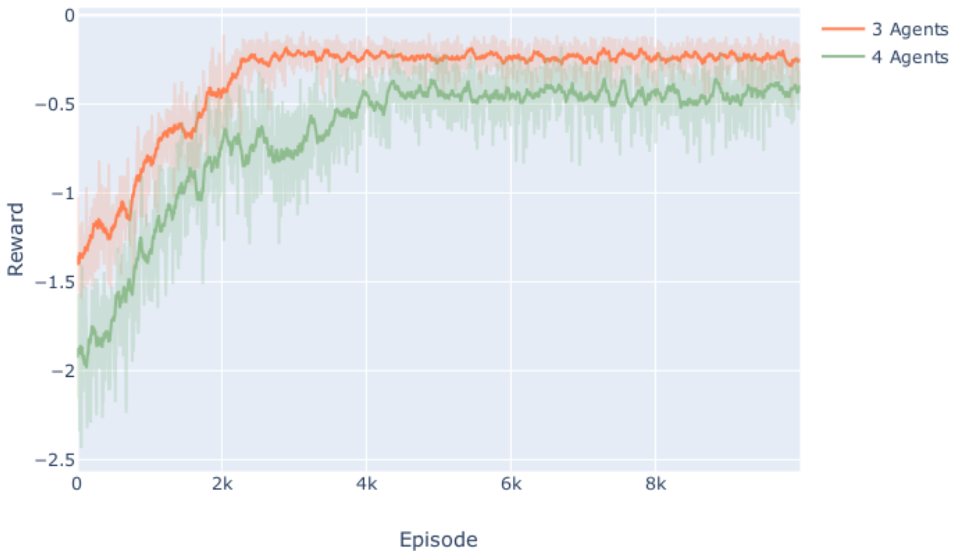
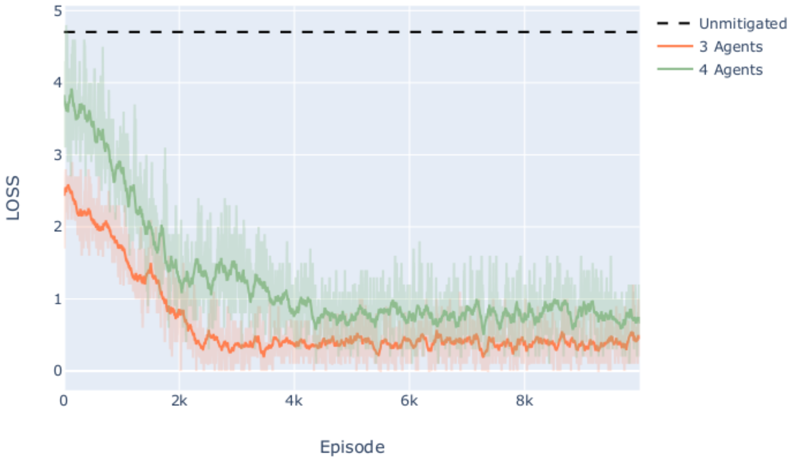
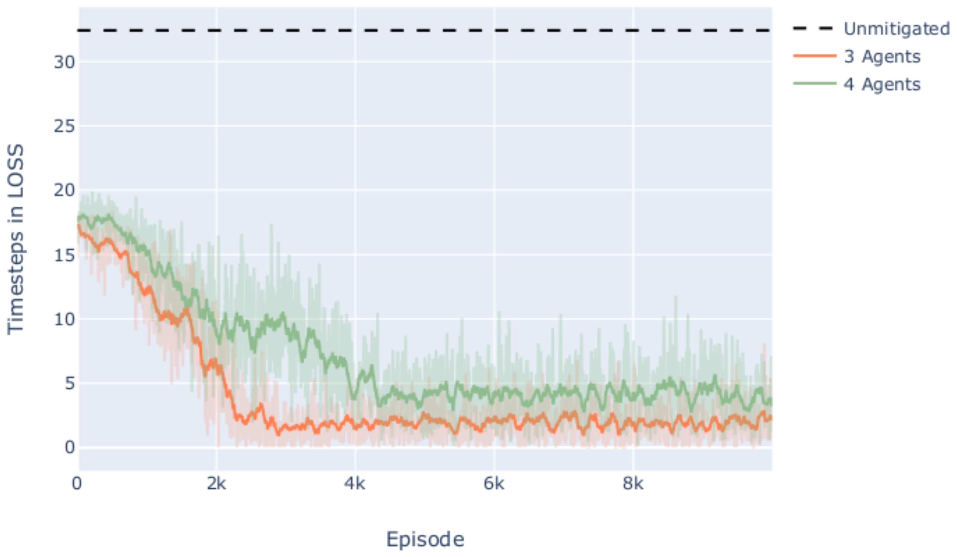
5. Simulation Results

5.1. Conflict Resolution Performance

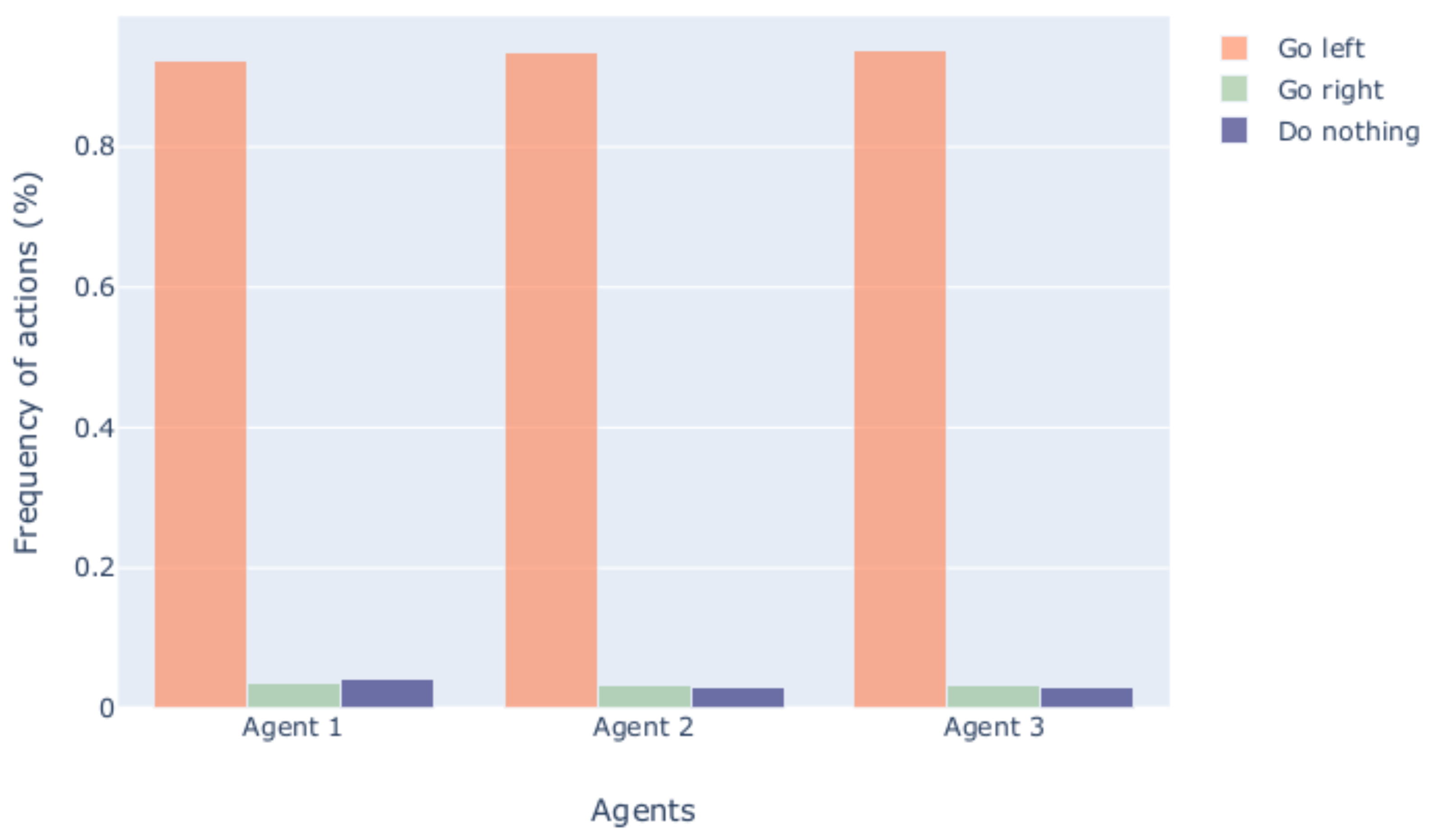
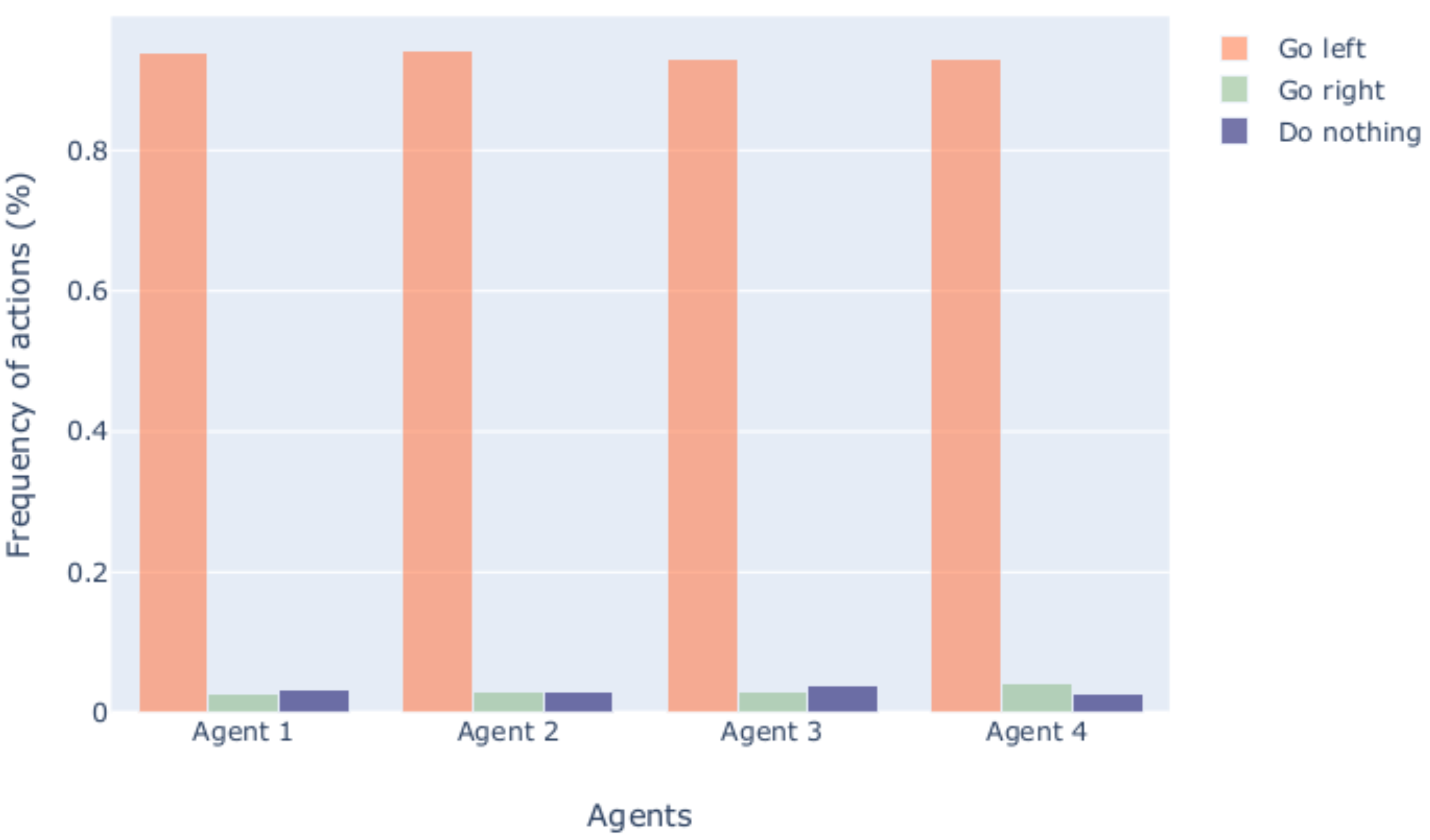
The model (the code can be found at https://github.com/risufaj/bluesky, accessed on 13 November 2021) was trained for 10,000 episodes with scenarios of compound conflicts with 3 UAVs. Then, it was trained for a further 10,000 episodes with scenarios of compound conflicts with 4 UAVs. In this way, we utilize the learned policies of the previous agents to fine-tune them in the four-agent case and train the new agent from scratch. The models were trained on the Google Cloud Platform (https://cloud.google.com, accessed on 13 November 2021) using an NVIDIA Tesla K80 GPU. The training lasted around 10 h.

Figure 1 shows the evolution of the cumulative reward for both cases. As the agents are cooperative, we are interested in the overall reward that is gained per episode and do not concern ourselves with the individual rewards. In this work, we utilize negative rewards, so the maximum the agents can get is 0. In the case of the 4 agents the reward seems a bit lower, however this comes a result of there being one more agent present, which takes actions to solve the conflicts thus inflicting itself some negative rewards for going away from track.

According to the figure, the model converges on both occasions. This means that the agents are successfully able to improve their policies with gained experience. However, in the case with 3 present agents, the convergence happens around 2000 episodes, while around 4000 episodes are required for the 4 agent case. In the latter case, there are more possible scenarios that can be generated, therefore increasing the variance of situations that the agents are presented with. Furthermore, in the beginning of training the already present agents employ their learned policies, while the new agent is exploring the possible actions, which reduces the overall reward the agents get.

In Figure 2 the number of losses of separation (LOSS) is shown. The number of LOSS of the average unmitigated case (for both 3 and 4 agents) is shown with the dashed line. The reward performance translates directly to successfully avoiding LOSS. In the case with 3 present agents, after convergence the average LOSS per episode is less than 1. This indicates that the agents are able to successfully solve conflicts before violating the self-separation distance. In the case of the 4 agents compound conflict, the average is around 1 LOSS per episode. However, through our results, we note that the model manages to always avoid near misses in both cases, as the NMAC distance is never breached.

We can observe a similar evolution in Figure 1, with the retrained model performing slightly worse. In general, the case with four agents had more pairwise conflicts present, which makes the problem more difficult.

Table 1. Number of episodes compound conflicts solved.

3 Agents	4 Agents
5650	4461

shows in how many episodes the compound conflict was solved, meaning no LOSS has occurred. The difference is similar to the number of extra epochs the 4 agents model needed to converge. As such, once the model converges it can generally manage to solve the compound conflict, thus fulfilling its task successfully. This result shows that the agents are able to solve conflicts through communicating with their neighbors.

In addition to solving conflicts, it is desirable for agents not to spend too much in a LOSS, as this can increase the risk of collisions. Such information is shown in Figure 3. The results shown there further confirm that the agents are able to improve their performance. In a similar trend, the case of the 3 agents compound conflict seems simpler to solve successfully, as the agents spend less than 5 s in a LOSS, with 5650 episodes not experiencing a LOSS (therefore no time steps in LOSS) Through the results presented in this section, RQ1 can be answered. In both problem settings, agents can improve and eventually solve the majority of conflicts. Furthermore, even in cases where there are still conflicts present at the end of an episode, we observe that there are no NMACs present. Nevertheless, an approach where hard-coded maneuvers (i.e., Collision Avoidance) as a second layer of safety can be included.

5.2. Agent Behavior

The results shown so far indicate that the agents manage to successfully learn how to solve the task. The model converges fast and maintains its knowledge of the system, thus avoiding the common forgetting issues.

However, it is important to understand what strategies they learned. This information is shown in Figure 4 and Figure 5. For the sake of simplicity, we only show the frequency of actions for the last 200 episodes.

We note that in both settings, the agents take the go left action in the majority of cases. While the direction of the action might not be as important, the learned strategy suggests that agents take the same action. This results in agents increasing the distance between them, as taking the same action head-on or crossing scenarios results in them going in different directions. However, in overtaking scenarios such a strategy does not immediately solve the conflict. Nevertheless, through the reward agents must learn that the conflict with the smallest CPA distance is the most urgent. As such, it can happen that agents prefer to delay the solution in an overtaking scenario, by taking several small changes in the same direction. While this is not immediately desirable, attempting to make a heading change to the opposite direction could create a more severe conflict with the head-on or crossing agents.

In this work, we do not put any restrictions to the agents and do not inject expert knowledge in them, thus they start learning from a blank state. The results show that the agents are able to learn a strategy that successfully solves the compound conflicts in scenarios with 3 and 4 agents. These results answer RQ2.

6. Conclusions and Future Work

In this paper, we tackle multi-UAV conflict resolution by modeling it as a MARL problem with cooperative agents. Air traffic is represented as a graph with aircraft as nodes. An edge is created between every two aircraft in a pairwise conflict. We use graph convolutional reinforcement learning, which provides a communication mechanism between connected agents. This means that conflicting aircraft are allowed to communicate with each other and develop cooperative strategies. To formally define a multi-UAV conflict, we propose the concept of compound conflicts, which are conflicts that have tight spatial and temporal boundaries.

We first train a model that learns how to solve compound conflicts with 3 agents. After that, the same model is retrained to to solve compound conflicts with 4 agents. As a result, we are able to refine the policies learned in the previous setting, while added agent learns a desirable policy.

Results show that the agents are able to improve their policies and thus solve the task. For both settings, we observe an improvement both in number of LOSS present and duration of LOSS with the majority of scenarios after convergence having no LOSS (i.e., the compound conflict is solved). Furthermore, the agents are able to discover a strategy that increases the overall distance between them. As such, they effectively learn to solve the most severe conflicts first and then solve the remaining conflicts while making sure that no new conflicts are created.

However, there are several aspects that must be further researched. For instance, in this work we use a maximum of 4 agents in the scenario. In reality, the number of agents in a compound conflict can not be always decided beforehand, thus a solution that adapts to $\mathcal{N}$ agents must be sought. Furthermore, the reward function could be further elaborated to include terms that deal with the quality of solutions, such as optimizing for battery usage or number of actions taken. Finally, the action space can be extended to include solutions by speed or altitude changes.

References

1. SESAR JU. European Drones Outlook Study; Single European Sky ATM Research; SESAR JU: Brussels, Belgium, 2016; p. 93. [Google Scholar]
2. Barrado, C.; Boyero, M.; Brucculeri, L.; Ferrara, G.; Hately, A.; Hullah, P.; Martin-Marrero, D.; Pastor, E.; Rushton, A.P.; Volkert, A. U-space concept of operations: A key enabler for opening airspace to emerging low-altitude operations. Aerospace 2020, 7, 24. [Google Scholar] [CrossRef] [Green Version]
3. Prevot, T.; Rios, J.; Kopardekar, P.; Robinson, J.E., III; Johnson, M.; Jung, J. UAS Traffic Management (UTM) Concept of Operations to Safely Enable Low Altitude Flight Operations. In Proceedings of the 16th AIAA Aviation Technology, Integration, and Operations Conference, Washington, DC, USA, 13–17 June 2016; pp. 1–16. [Google Scholar] [CrossRef]
4. Zhang, J. UOMS in China. In Proceedings of the EU-China APP Drone Workshop, Shenzhen, China, 6–8 June 2018; pp. 6–8. [Google Scholar]
5. UTM—A Common Framework with Core Principles for Global Harmonization. Available online: https://www.icao.int/safety/UA/Documents/UTM%20Framework%20Edition%203.pdf (accessed on 11 October 2021).
6. NASA Conflict Management Model. Available online: https://www.nasa.gov/sites/default/files/atoms/files/2020-johnson-nasa-faa.pdf (accessed on 11 October 2021).
7. Radanovic, M.; Omeri, M.; Piera, M.A. Test analysis of a scalable UAV conflict management framework. Proc. Inst. Mech. Eng. Part G J. Aerosp. Eng. 2019, 233, 6076–6088. [Google Scholar] [CrossRef]
8. Consiglio, M.; Muñoz, C.; Hagen, G.; Narkawicz, A.; Balachandran, S. ICAROUS: Integrated configurable algorithms for reliable operations of unmanned systems. In Proceedings of the 2016 IEEE/AIAA 35th Digital Avionics Systems Conference (DASC), Sacramento, CA, USA, 25–29 September 2016; pp. 1–5. [Google Scholar] [CrossRef] [Green Version]
9. Johnson, S.C.; Petzen, A.N.; Tokotch, D.S. Johnson_DetectAndAvoid Aviation 2017 Handout. 2017. Available online: https://nari.arc.nasa.gov/sites/default/files/Johnson_DetectAndAvoid%20Aviation%202017%20Handout.pdf (accessed on 11 October 2021).
10. Manfredi, G.; Jestin, Y. Are You Clear About ” Well Clear ”? In Proceedings of the 2018 International Conference on Unmanned Aircraft Systems (ICUAS), Dallas, TX, USA, 12–15 June 2018; pp. 599–605. [Google Scholar]
11. Cook, B.; Arnett, T.; Cohen, K. A Fuzzy Logic Approach for Separation Assurance and Collision Avoidance for Unmanned Aerial Systems. In Modern Fuzzy Control Systems and Its Applications; InTech: Rijeka, Croatia, 2017; pp. 1–32. [Google Scholar] [CrossRef] [Green Version]
12. Consiglio, M.; Duffy, B.; Balachandran, S.; Glaab, L.; Muñoz, C. Sense and avoid characterization of the independent configurable architecture for reliable operations of unmanned systems. In Proceedings of the 13th USA/Europe Air Traffic Management Research and Development Seminar 2019, Vienna, Austria, 17–21 June 2019. [Google Scholar]
13. Muñoz, C.A.; Dutle, A.; Narkawicz, A.; Upchurch, J. Unmanned aircraft systems in the national airspace system: A formal methods perspective. ACM SIGLOG News 2016, 3, 67–76. [Google Scholar] [CrossRef] [Green Version]
14. Weinert, A.; Campbell, S.; Vela, A.; Schuldt, D.; Kurucar, J. Well-clear recommendation for small unmanned aircraft systems based on unmitigated collision risk. J. Air Transp. 2018, 26, 113–122. [Google Scholar] [CrossRef] [Green Version]
15. McLain, T.W.; Duffield, M.O. A Well Clear Recommendation for Small UAS in High-Density, ADS-B-Enabled Airspace. In Proceedings of the AIAA Information Systems-AIAA Infotech @ Aerospace, Grapevine, TX, USA, 9–13 January 2017. [Google Scholar]
16. Modi, H.C.; Ishihara, A.K.; Jung, J.; Nikaido, B.E.; D’souza, S.N.; Hasseeb, H.; Johnson, M. Applying Required Navigation Performance Concept for Traffic Management of Small Unmanned Aircraft Systems. In Proceedings of the 30th Congress of the International Council of the Aeronautical Sciences, Daejeon, Korea, 25–30 September 2016. [Google Scholar]
17. Jiang, J.; Dun, C.; Huang, T.; Lu, Z. Graph convolutional reinforcement learning. arXiv 2018, arXiv:1810.09202. [Google Scholar]
18. Skowron, M.; Chmielowiec, W.; Glowacka, K.; Krupa, M.; Srebro, A. Sense and avoid for small unmanned aircraft systems: Research on methods and best practices. Proc. Inst. Mech. Eng. Part G J. Aerosp. Eng. 2019, 233, 6044–6062. [Google Scholar] [CrossRef]
19. Kuchar, J.K.; Yang, L.C. A review of conflict detection and resolution modeling methods. IEEE Trans. Intell. Transp. Syst. 2000, 1, 179–189. [Google Scholar] [CrossRef] [Green Version]
20. Ribeiro, M.; Ellerbroek, J.; Hoekstra, J. Review of conflict resolution methods for manned and unmanned aviation. Aerospace 2020, 7, 79. [Google Scholar] [CrossRef]
21. Bertram, J.; Wei, P. Distributed computational guidance for high-density urban air mobility with cooperative and non-cooperative collision avoidance. In Proceedings of the AIAA Scitech 2020 Forum, Orlando, FL, USA, 6–10 January 2020; p. 1371. [Google Scholar]
22. Yang, X.; Wei, P. Scalable multiagent computational guidance with separation assurance for autonomous urban air mobility. J. Guid. Control Dyn. 2020, 43, 1473–1486. [Google Scholar] [CrossRef]
23. Hu, J.; Yang, X.; Wang, W.; Wei, P.; Ying, L.; Liu, Y. UAS Conflict Resolution in Continuous Action Space Using Deep Reinforcement Learning. In Proceedings of the AIAA Aviation 2020 Forum, Virtual Event, 15–19 June 2020; p. 2909. [Google Scholar]
24. Ribeiro, M.; Ellerbroek, J.; Hoekstra, J. Determining Optimal Conflict Avoidance Manoeuvres At High Densities With Reinforcement Learning. In Proceedings of the 10th SESAR Innovation Days, Virtual Event, 7–10 December 2020. [Google Scholar]
25. Isufaj, R.; Aranega Sebastia, D.; Piera, M.A. Towards Conflict Resolution with Deep Multi-Agent Reinforcement Learning. In Proceedings of the 14th USA/Europe Air Traffic Management Research and Development Seminar (ATM2021), New Orleans, LA, USA, 20–24 September 2021. [Google Scholar]
26. Lowe, R.; Wu, Y.; Tamar, A.; Harb, J.; Abbeel, P.; Mordatch, I. Multi-agent actor-critic for mixed cooperative-competitive environments. arXiv 2017, arXiv:1706.02275. [Google Scholar]
27. Pham, D.T.; Tran, N.P.; Alam, S.; Duong, V.; Delahaye, D. A machine learning approach for conflict resolution in dense traffic scenarios with uncertainties. In Proceedings of the ATM Seminar 2019, 13th USA/Europe ATM R&D Seminar, Vienna, Austria, 7–21 June 2019. [Google Scholar]
28. Brittain, M.; Yang, X.; Wei, P. A deep multiagent reinforcement learning approach to autonomous separation assurance. arXiv 2020, arXiv:2003.08353. [Google Scholar]
29. Dalmau, R.; Allard, E. Air Traffic Control Using Message Passing Neural Networks and Multi-Agent Reinforcement Learning. In Proceedings of the 10th SESAR Innovation Days, Virtual Event, 7–10 December 2020. [Google Scholar]
30. Manfredi, G.; Jestin, Y. An introduction to ACAS Xu and the challenges ahead. In Proceedings of the 2016 IEEE/AIAA 35th Digital Avionics Systems Conference (DASC), Sacramento, CA, USA, 25–29 September 2016; pp. 1–9. [Google Scholar]
31. Sutton, R.S.; Barto, A.G. Introduction to Reinforcement Learning; MIT Press: Cambridge, MA, USA, 1998; Volume 135. [Google Scholar]
32. Lee, J.B.; Rossi, R.A.; Kim, S.; Ahmed, N.K.; Koh, E. Attention models in graphs: A survey. ACM Trans. Knowl. Discov. Data (TKDD) 2019, 13, 1–25. [Google Scholar] [CrossRef] [Green Version]
33. Hernandez-Leal, P.; Kartal, B.; Taylor, M.E. A survey and critique of multiagent deep reinforcement learning. Auton. Agents Multi-Agent Syst. 2019, 33, 750–797. [Google Scholar] [CrossRef] [Green Version]
34. Bellman, R. Dynamic programming and stochastic control processes. Inf. Control 1958, 1, 228–239. [Google Scholar] [CrossRef] [Green Version]
35. François-Lavet, V.; Henderson, P.; Islam, R.; Bellemare, M.G.; Pineau, J. An introduction to deep reinforcement learning. arXiv 2018, arXiv:1811.12560. [Google Scholar]
36. Mnih, V.; Kavukcuoglu, K.; Silver, D.; Graves, A.; Antonoglou, I.; Wierstra, D.; Riedmiller, M. Playing atari with deep reinforcement learning. arXiv 2013, arXiv:1312.5602. [Google Scholar]
37. Littman, M.L. Markov games as a framework for multiagent reinforcement learning. In Machine Learning Proceedings 1994, Proceedings of the Eleventh International Conference, Rutgers University, New Brunswick, NJ, USA, 10–13 July 1994; Elsevier: Amsterdam, The Netherlands, 1994; pp. 157–163. [Google Scholar]
38. Wu, Z.; Pan, S.; Chen, F.; Long, G.; Zhang, C.; Philip, S.Y. A comprehensive survey on graph neural networks. IEEE Trans. Neural Netw. Learn. Syst. 2020, 32, 4–24. [Google Scholar] [CrossRef] [Green Version]
39. Veličković, P.; Cucurull, G.; Casanova, A.; Romero, A.; Lio, P.; Bengio, Y. Graph attention networks. arXiv 2017, arXiv:1710.10903. [Google Scholar]
40. Kipf, T.N.; Welling, M. Semi-supervised classification with graph convolutional networks. arXiv 2016, arXiv:1609.02907. [Google Scholar]
41. Gilmer, J.; Schoenholz, S.S.; Riley, P.F.; Vinyals, O.; Dahl, G.E. Neural message passing for quantum chemistry. In Proceedings of the International Conference on Machine Learning, PMLR, Sydney, Australia, 6–11 August 2017; pp. 1263–1272. [Google Scholar]
42. Zambaldi, V.; Raposo, D.; Santoro, A.; Bapst, V.; Li, Y.; Babuschkin, I.; Tuyls, K.; Reichert, D.; Lillicrap, T.; Lockhart, E.; et al. Relational deep reinforcement learning. arXiv 2018, arXiv:1806.01830. [Google Scholar]
43. Koca, T.; Isufaj, R.; Piera, M.A. Strategies to Mitigate Tight Spatial Bounds Between Conflicts in Dense Traffic Situations. In Proceedings of the 9th SESAR Innovation Days, Athens, Greece, 2–5 December 2019. [Google Scholar]
44. Hoekstra, J.M.; Ellerbroek, J. Bluesky ATC simulator project: An open data and open source approach. In Proceedings of the 7th International Conference on Research in Air Transportation, FAA/Eurocontrol USA/Europe, Philadelphia, PA, USA, 20–24 June 2016; Volume 131, p. 132. [Google Scholar]
45. Shi, K.; Cai, K.; Liu, Z.; Yu, L. A Distributed Conflict Detection and Resolution Method for Unmanned Aircraft Systems Operation in Integrated Airspace. In Proceedings of the 2020 AIAA/IEEE 39th Digital Avionics Systems Conference (DASC), San Antonio, TX, USA, 11–15 October 2020; pp. 1–9. [Google Scholar] [CrossRef]
46. Mullins, M.; Holman, M.W.; Foerster, K.; Kaabouch, N.; Semke, W. Dynamic Separation Thresholds for a Small Airborne Sense and Avoid System. In Proceedings of the AIAA Infotech@Aerospace (I@A) Conference, Boston, MA, USA, 19–22 August 2013. [Google Scholar]
47. Ho, F.; Geraldes, R.; Alves Gonçalves, A.; Cavazza, M.; Prendinger, H. Improved Conflict Detection and Resolution for Service UAVs in Shared Airspace. IEEE Trans. Veh. Technol. 2018, 68, 1231–1242. [Google Scholar] [CrossRef]
48. Johnson, S.C.; Petzen, A.N.; Tokotch, D.S. Exploration of Detect-and-Avoid and Well-Clear Requirements for Small UAS Maneuvering in an Urban Environment. In Proceedings of the 17th AIAA Aviation Technology, Integration, and Operations Conference, Denver, CO, USA, 5–9 June 2017. [Google Scholar]
Figure 1. Evolution of cumulative reward per episode.
Applsci 12 00610 g001
Figure 2. Number of losses of separation in comparison with average unmitigated case.
Applsci 12 00610 g002
Figure 3. Number of time steps spent in LOSS.
Applsci 12 00610 g003
Figure 4. Frequency of actions for last 200 episodes of compound conflict with 3 agents.
Applsci 12 00610 g004
Figure 5. Frequency of actions for last 200 episodes of compound conflict with 4 agents.
Applsci 12 00610 g005