Design and Optimization of a Neuro-Fuzzy System for the Control of an Electromechanical Plant

Abstract

One characteristic of neuro-fuzzy systems is the possibility of incorporating preliminary information in their structure as well as being able to establish an initial configuration to carry out the training. In this regard, the strategy to establish the configuration of the fuzzy system is a relevant aspect. This document displays the design and implementation of a neuro-fuzzy controller based on Boolean relations to regulate the angular position in an electromechanical plant, composed by a motor coupled to inertia with friction (a widely studied plant that serves to show the control system design process). The structure of fuzzy systems based on Boolean relations considers the operation of sensors and actuators present in the control system. In this way, the initial configuration of fuzzy controller can be determined. In order to perform the optimization of the neuro-fuzzy controller, the continuous plant model is converted to discrete time to be included in the closed-loop controller training equations. For the design process, first the optimization of a Proportional Integral (PI) linear controller is carried out. Thus, linear controller parameters are employed to establish the structure and initial configuration of the neuro-fuzzy controller. The optimization process also includes weighting factors for error and control action in such a way that allows having different system responses. Considering the structure of the control system, the optimization algorithm (training algorithm) employed is dynamic back propagation. The results via simulations show that optimization is achieved in the linear and neuro-fuzzy controllers using different weighting values for the error signal and control action. It is also observed that the proposed control strategy allows disturbance rejection.

1. Introduction

In control systems, fuzzy logic offers broad applicability given its flexibility to implement control strategies through a set of rules using membership functions [1,2,3]. It is possible to use training algorithms with neural networks when representing the fuzzy system as a neural network that grants higher accuracy in the fuzzy system performance. When representing a fuzzy system as a neural network, a neuro-fuzzy system is obtained [4,5].

An interesting application of fuzzy logic is the aided design process. In this regard, a remarkable application is observed for compliant mechanism design used in soft robotics, space, and bioengineering due to the advantages of free friction, monolithic structure, and minimal assembly. Considering this area, a hybrid methodology is presented in [6] for solving the multi-objective optimization design. Authors propose a hybridization through a combination of a finite element method, statistical technique, desirability function approach, fuzzy logic system, Adaptive Neuro-Fuzzy Inference System (ANFIS), and Lightning Attachment Procedure Optimization (LAPO). A bistable compliant mechanism is designed, where desirability values of two performance metrics are calculated and transferred into the fuzzy logic system to obtain the output in a single objective function. A related work is presented in [7], proposing a method using statistics, numerical simulation, computational intelligence, and metaheuristics. A two-degree of freedom compliant mechanism is designed, where numerical datasets are collected by simulations. The sensitivity of design parameters is studied by analysis of variance and Taguchi technique. The results of sensitivity are employed to separate populations for lightning attachment procedure optimization. The values of two output mechanism performances are the inputs of the fuzzy logic model, and the output of this system is a single objective function, that is optimized using LAPO algorithm. Other advanced work is presented in [8], presenting an optimization framework to provide a systematic design method for a flexure gripper. The optimization strategy includes the topology, modeling, and size optimization phases. The gripper topology is determined via the solids isotropic material with penalization method considering stress constraint and force distribution. The modeling of the performances is implemented via an Enhanced Adaptive Neuro-Fuzzy Inference System (EANFIS). The optimization is performed to search for the best model parameters. Finally, a hybrid procedure of the Taguchi method is described in [9], using fuzzy logic, response surface method, and Moth-flame optimization algorithm to solve the design optimization of a flexure hinge to enhance three quality characteristics. Fuzzy modeling is proposed to interpolate the three objective functions into a unified objective function. An integrated regression equation is determined via response surface method and flexure hinge is optimized using Moth-flame optimization algorithm.

Regarding fuzzy control applications for electromechanical systems, there are relevant developments in electric engines control and robotics. With regard to fuzzy logic for motor control, reference [10] carries out a review of multi-motor control, which are multiple input and multiple output systems. The main purpose of the multiple motor control variators consists of achieving a coordinated operation in all motors. The literature reviewed shows that fuzzy systems are widely employed in multi-motor control. Meanwhile, in [11] a fuzzy controller is proposed using a motion capture system to operate the speed and orientation of a wheelchair considering the model of a Direct Current (DC) motor for the design process. Further, a fuzzy logic controller is used in [12], for an image-based navigation system of an autonomous underwater vehicle with a DC motor.

According to [13], due to high robustness and simple maintenance, Induction Motors (IM) are commonly used in household appliances and industries. Currently, advanced techniques are applied to traditional controls such as the Field-Oriented Control (FOC) and Direct Torque Control (DTC). Authors in [13] evaluate traditional FOC and DTC compared to two additional fuzzy and predictive controllers.

Concerning robotic applications using fuzzy logic, reference [14] employs a fuzzy control Proportional Integral (PI) in a robotic driving system for hybrid electric vehicles in a way that allows a reliable evaluation of energy efficiency. This depicts the relevance of the efficiency of fuel in hybrid vehicles. Thus, reliable measurements are required in order to have an accurate analysis of fuel efficiency; whereby, the authors propose a robotic system to perform driving tests to reduce the deviation when such tests are carried out by humans. Moreover, reference [15] proposes a Knowledge-Based Neural Fuzzy Controller (KNFC) for navigation control in mobile robots. Knowledge-Based Cultural Multi-Strategy Differential Evolution (KCMDE) is employed here to adjust the parameters of the KNFC. This is applied in mobile robots PIONEER 3-DX for automatic navigation systems and obstacle avoidance, employing the existing angle between the obstacle and the robot to determine if the robot enters in specific reference points to modify its behavior and thus skip dead ends. A related work is presented in [16] using a neuro-fuzzy system in path planning for a service robot in complex environments with the presence of humans as in a retirement home. As inputs for path planning, the system uses a 3D depth camera and multiple sonar sensors.

Meanwhile, reference [17] proposes a simple and practical decoupled control structure for a parallel robot positioning control using the Cable-Driven Parallel Robot (CDPR). This structure is employed with a non-linear Proportional Integral Derivative (PID) and classic PID controllers. In addition, the control system structure is proposed through an analysis of cables involved in End-Effector (EE) robot’s movement when operating independently for each axis; later, an adjustment of rules for fuzzy PID controllers was carried out and the Ziegler–Nichols method was applied to PID classic controllers.

Regarding recent research of neuro-fuzzy control systems, in [18] is developed a Terminal Sliding-Mode Control (TSMC) using a Fuzzy Double Hidden Layer Recurrent Neural Network (FDHLRNN). According to authors, the neuro-fuzzy system proposed is a combination of a radial basis neural network and a fuzzy neural network. To reduce the switching gain (associated with the TSMC), the FDHLRNN is employed to approximate the nonlinear sliding-mode equivalent control term. In order to observe the dynamic response and robustness, the control scheme is tested using a second-order nonlinear system. An additional work is observed in [19], where is designed a TSMC using FDHLRNN for a single-phase Active Power Filter (APF). Authors propose the TSMC to allow the tracking error converges to zero (in a finite time). The system is used in harmonic suppression first to approximate the equivalent control and second to suppress unknown disturbances. The equations to update the adaptive parameters of the FDHLRNN are obtained using a Liapunov function in order to ensure asymptotic stability. Finally, in [20] is displayed an approximation-based adaptive fractional sliding mode control. For approximating the system uncertainties and disturbance we used a Double Loop Recurrent Fuzzy Neural Network (DLRFNN). In this development, a fractional order term is incorporated into the sliding surface having the benefits of sliding mode control and fractional calculus. The DLRFNN uses the advantages of fuzzy systems to handle uncertain information and the neural networks to learn using data measured from the process.

In this work, the designed neuro-fuzzy controller uses the structure of a compact fuzzy system based on Boolean relations as presented in [21], which can be used for the identification and control of dynamic systems. Neuro-fuzzy systems based on Boolean relations are founded in a system design considering possible Boolean regions in the universe discourse, then being extended using fuzzy sets for implementation [22]. Various design considerations are presented in this scenario as well as the manipulation of system equations applying Boole and Kleene algebras. In this way, fuzzy systems with compact structures can be established and used for identification and control of dynamic systems [21]. As an example, the application of this type of system is shown in [23] to control an Automatic Voltage Regulator (AVR). In control applications, the Dynamic Back Propagation (DBP) training algorithm is used in cases when the plant’s feedback signals and the controller are required for the neuro-fuzzy control system.

This document details the design and tuning of a neuro-fuzzy control system applied to an electromechanical plant. The neuro-fuzzy system design is made regarding the architecture of a linear controller. Subsequently, the training is performed similar to a neural network employing the dynamic back propagation algorithm [24,25,26].

The design can be applied in robotics since it is necessary to control the movements of the parts of a robot which are generally activated with DC motors. Another application can be a solar tracker usually employed to improve the use of solar energy. In previous works, the considered plant is similar to that employed to control a solar tracker mainly operated by a DC motor [27,28,29]. Regarding this plant, reference [30] carries out the optimization of a linear controller in discrete time.

Article Approach and Document Organization

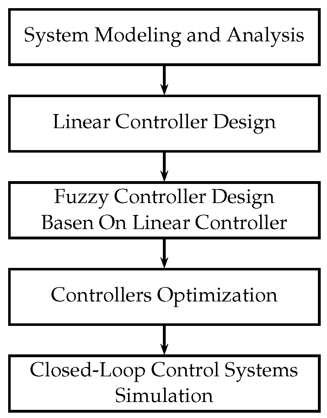
The objective of this document is to show the design and optimization process of a fuzzy controller (based on Boolean relations), making the equivalence with a linear controller, for which a well-known plant (widely studied) is used to show the design process and optimization. Considering this work, the design process can be extended to more complex plants. Moreover, this document considers the design of a linear controller as reference since it allows determining the structure of the fuzzy controller as well as its initial configuration, which also allows the optimization using the dynamic back propagation algorithm where the equations in closed-loop are deduced to train the linear and fuzzy controllers. The values from the linear controller are used to determine the initial configuration to optimize the fuzzy controller. A well-known plant composed of a coupled motor with a gear box and inertia with friction is employed to exhibit the design process and training of the controller. From the above, Figure 1 displays the methodology employed. First, the system modeling and analysis is performed, then the linear controller design used as the basis for designing the fuzzy controller (as mentioned above) is conducted. Later, the optimization of the controllers is carried out and finally the simulation of the closed-loop control system is performed.

The document is organized as follows: Section 2 describes the plant model considering a simplified structure and the representation in discrete time. Then, in Section 3 the description is shown of the linear and fuzzy controllers employed. Section 4 displays the general process for controller parameter training. Section 5 describes the equations for linear controller parameter training and Section 6 the equations for fuzzy controller optimization. Then, Section 7 presents the results of the controller training process. Finally, Section 8 shows the discussion and conclusions are presented in Section 9.

2. Electromechanical Plant

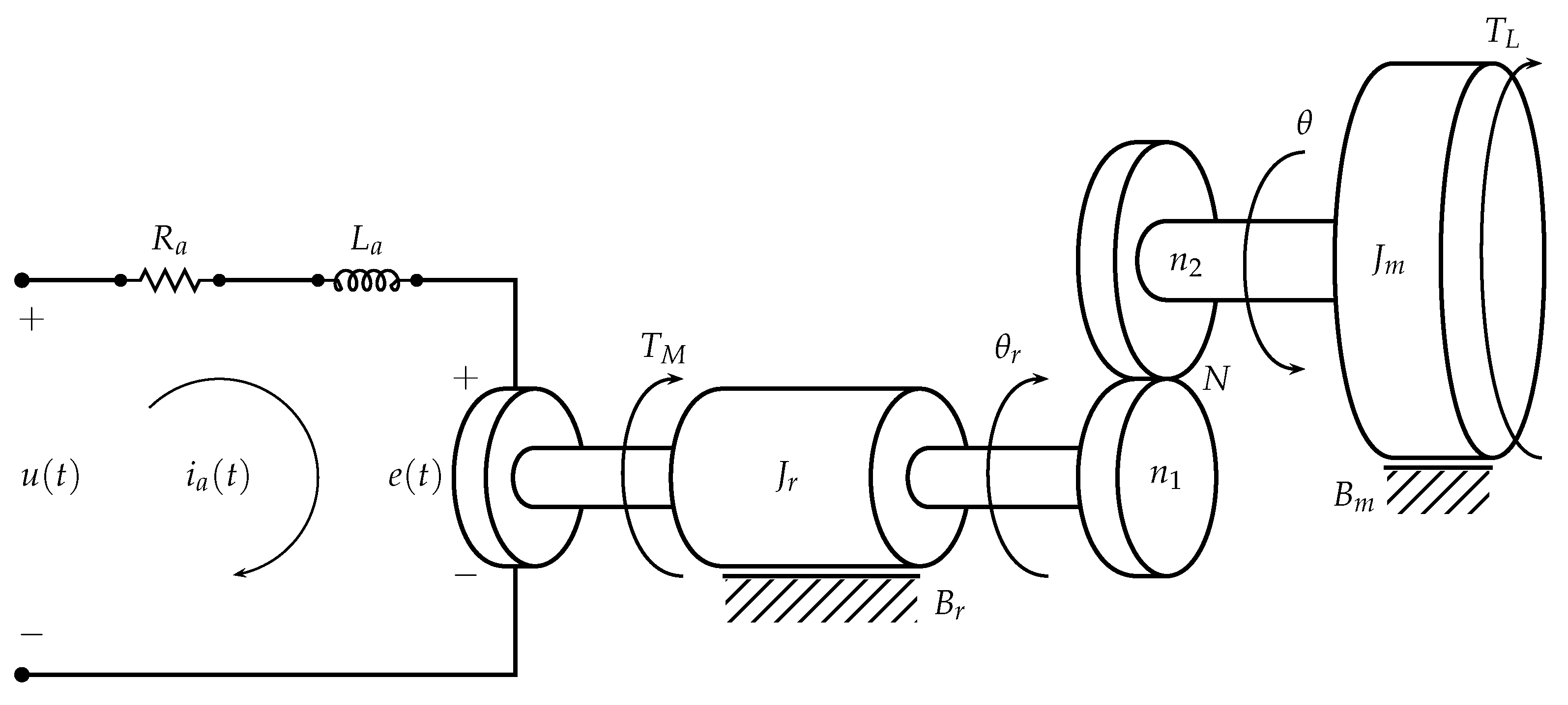
Figure 2 displays the diagram of the electromechanical plant considered. This is composed of a DC motor, a gearbox, and a wheel (with moment of inertia) coupled to the gearbox. The analysis of this plant is presented in [31], corresponding to the example A-3-9 pages 95–97. The motor plays an important role in this plant since it is a fundamental part of the dynamic model, as it provides the required torque to move the inertia. The parameters of the DC motor are:

• $K_t$: Torque constant.
• $K_e$: Electromagnetic feedback constant.
• $R_a$: Shield resistance.
• $L_a$: Shield inductance.
• $J_r$: Motor moment of inertia.
• $B_r$: Rotor friction constant.

It is noteworthy that the diagram in Figure 2 is given as an example since in a real case the gearbox has more gears. The motor torque is proportional to the current of the shield for the modeling of the system as indicated in the following equation:

$$T_M=K_t{i}_a\left(t\right)$$

(1)

The counter-electromotive force is proportional to the angular speed of the motor:

$$e\left(t\right)=K_e{\omega }_r\left(t\right)$$

(2)

The equation that governs the electrical part is:

$$u\left(t\right)-e\left(t\right)=L_a\frac{d{i}_a\left(t\right)}{dt}+R_a{i}_a\left(t\right)$$

(3)

The torques in the motor shaft are considered to incorporate the mechanical part into the model. The relation between the generated torque and the load torque is obtained by performing a summation of torques on the motor shaft as shown below:

$$T_M\left(t\right)-N{T}_L\left(t\right)=J_e\frac{d{\omega }_r\left(t\right)}{dt}+B_e{\omega }_r\left(t\right)$$

(4)

where:

$$B_e=B_r+B_m{N}^2;J_e=J_r+J_m{N}^2;N=\frac{n_1}{n_2}$$

(5)

In these equations $J_m$, $B_m$ are the inertia and friction of the mechanical part and N the transformation ratio of the gearbox such that $\theta \left(t\right)=N{\theta }_r\left(t\right)$. In addition, Equation (6) is employed to complete the model.

$${\omega }_r=\frac{d{\theta }_r\left(t\right)}{dt}$$

(6)

2.1. System Block Diagram

In order to observe the presentation of this system as a transfer function, a Laplace transform $\mathcal{L}$ is applied, obtaining:

$$\begin{array}{ccc}\hfill T_M\left(s\right)& =& K_t{I}_a\left(s\right)\hfill \end{array}$$

(7)

$$\begin{array}{ccc}\hfill E\left(s\right)& =& K_e{\Omega }_r\left(s\right)\hfill \end{array}$$

(8)

$$\begin{array}{ccc}\hfill U\left(s\right)-E\left(s\right)& =& (R_a+s{L}_a)I_a\left(s\right)\hfill \end{array}$$

(9)

$$\begin{array}{ccc}\hfill T_M\left(s\right)-N{T}_L\left(s\right)& =& (B_e+s{J}_e){\Omega }_r\left(s\right)\hfill \end{array}$$

(10)

$$\begin{array}{ccc}\hfill {\Theta }_r\left(s\right)& =& \frac{{\Omega }_r\left(s\right)}{s}\hfill \end{array}$$

(11)

In addition, taking $T_L=0$ and $\Theta \left(s\right)=N{\Theta }_r\left(s\right)$ the system transfer function is:

$$\frac{\Theta \left(s\right)}{U\left(s\right)}=\frac{N{K}_t}{K_t{K}_{e}s+(L_{a}s+R_a)(J_{e}s+B_e)s}$$

(12)

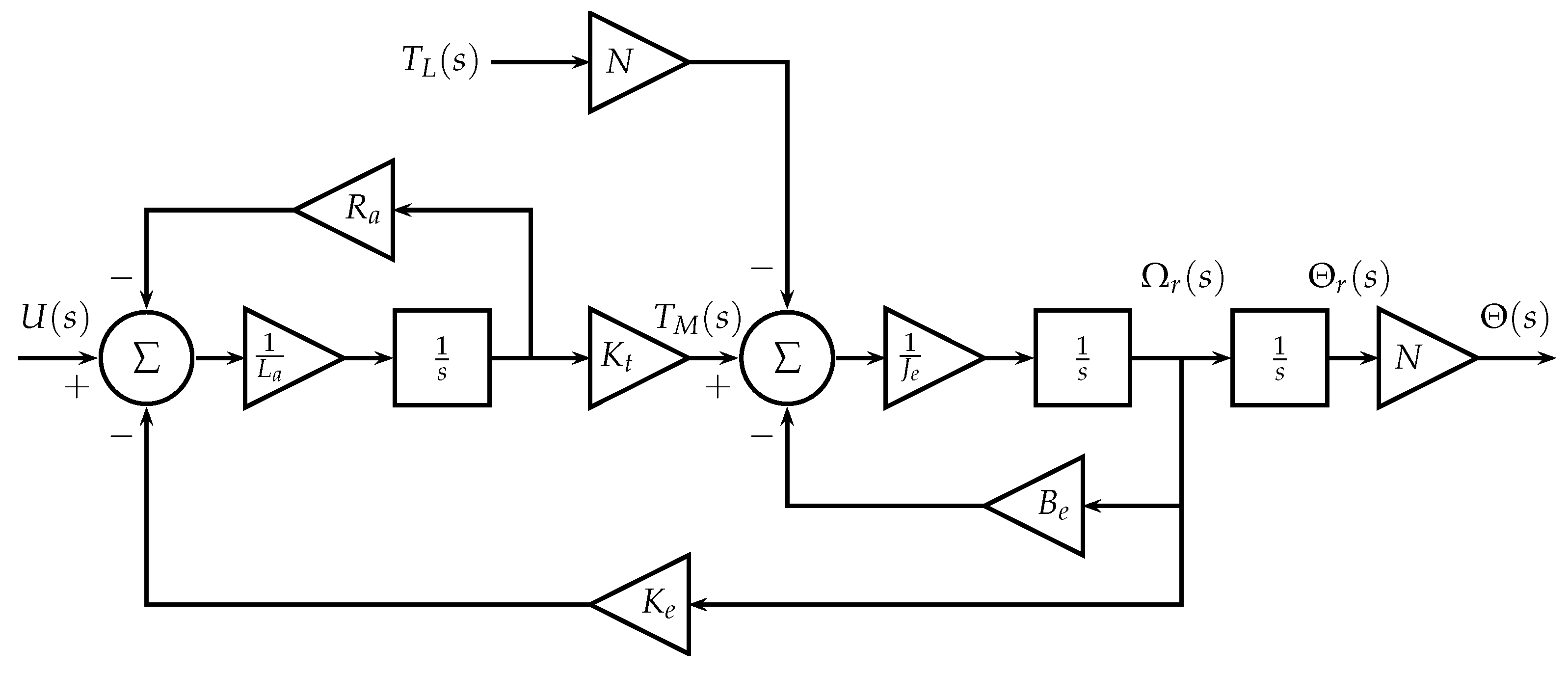
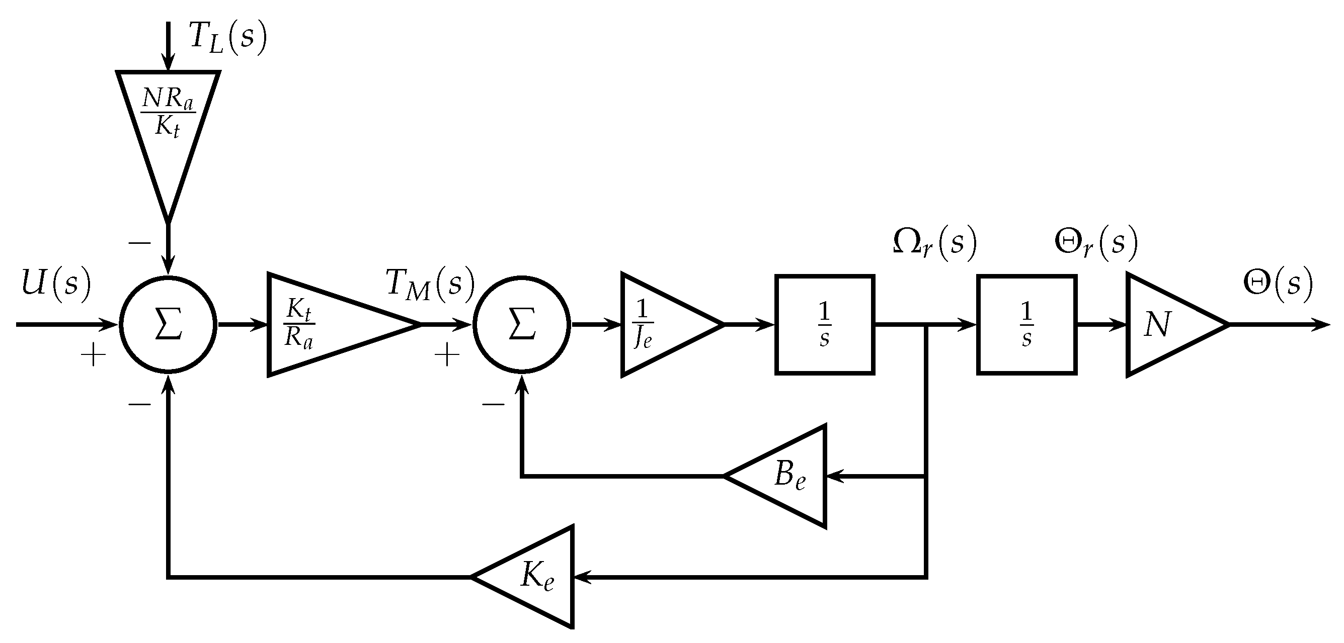
Considering the model equations, the block diagram in Figure 3 of the electromechanical system can be obtained.

2.2. Approximate Model

In some applications, a complete dynamic model of the plant may be impractical due to the difficulty in establishing the values of its parameter (in this case, the moment of inertia and the friction of the mechanical part). An alternative consists of a simplified model identifying its parameters considering the dynamic behavior of the plant [31].

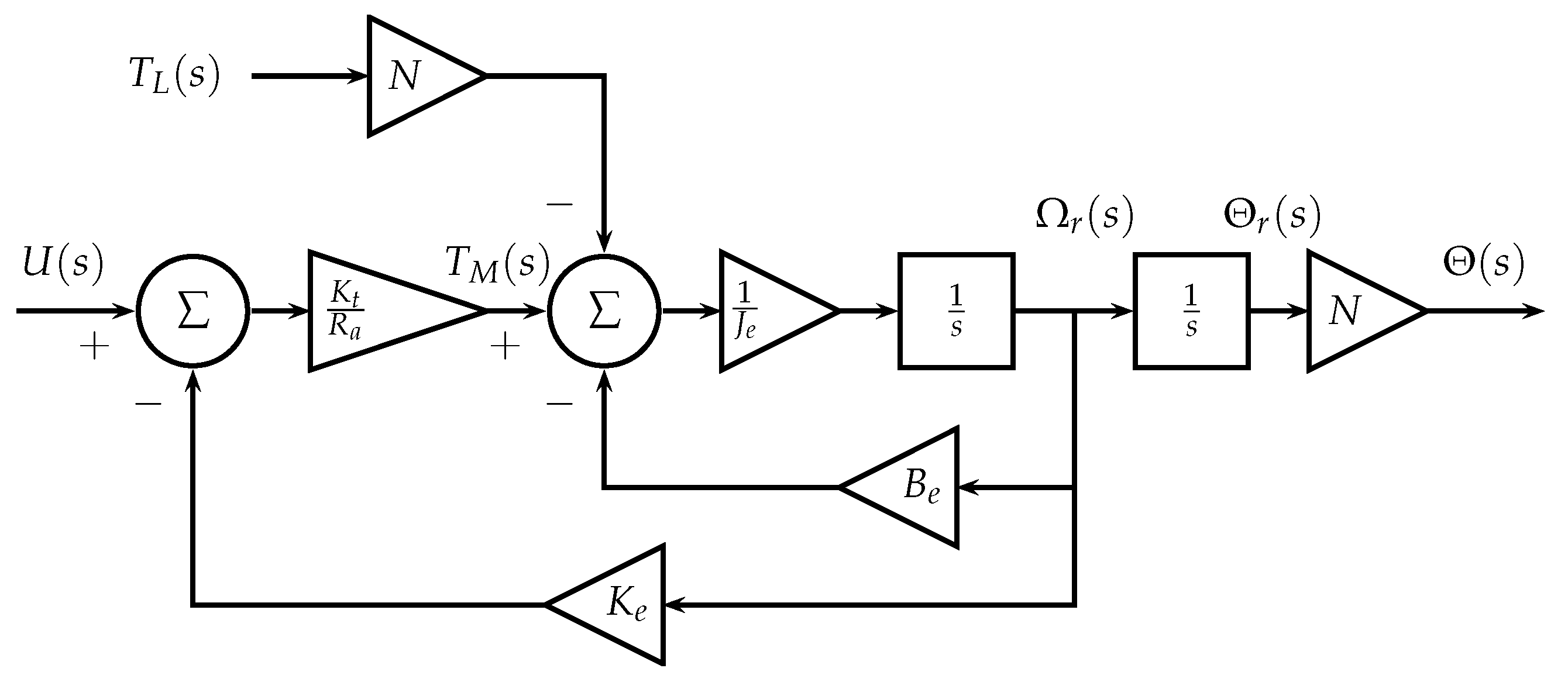
According to [31], when considering $L_a\approx 0$ (very small) there is a simplified model of the plant; in this way, the diagram in Figure 3 can be represented as shown in Figure 4.

Organizing the diagram of Figure 4, it is possible to obtain the representation of Figure 5 where $T_L\left(s\right)$ can be seen as a system disturbance.

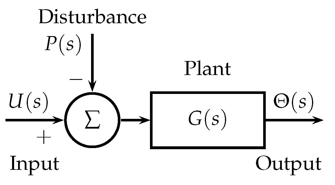
Equivalently, the diagram shown in Figure 6 is obtained where in the time domain the input $u\left(t\right)={\mathcal{L}}^{-1}\left\{U\left(s\right)\right\}$ corresponds to the voltage; the output is the angular position $\theta \left(t\right)={\mathcal{L}}^{-1}\{\Theta \left(s\right)\}$ and $p\left(t\right)={\mathcal{L}}^{-1}\left\{P\left(s\right)\right\}$ is the disturbance given by the product $(N{R}_a/K_t)T_L\left(t\right)$. In this way, the variable to sense and control corresponds to the angular position $\theta \left(t\right)$.

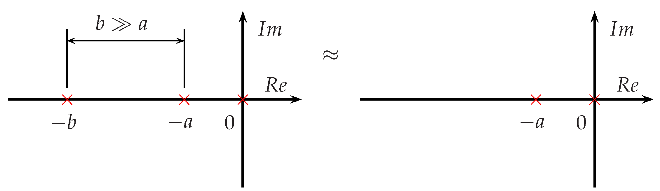
On the other hand, considering the location of the poles, the criterion to establish the simplified model is shown in Figure 7 where the pole located in $s=-a$ corresponding to the mechanical part is the dominant pole (it governs the system dynamics) since $b\gg a$; therefore, to establish the approximate model, the pole located at $s=-b$ associated with the electromagnetic part can be neglected [31].

Equation (13) describes the simplified plant transfer function corresponding to a first-order system and an integrator, where the variable s is associated with the Laplace transform.

According to [31], the model of Equation (13) considers the parameters shown in Figure 5, namely $J_e$, $B_e$, $K_e$, $K_t$, N, and $R_a$. In this way, through the data measured from the open-loop plant, the effect of the parameters on the plant operation is being directly considered in the identification process.

$$G\left(s\right)=\frac{K}{s(\tau s+1)}$$

(13)

For this plant, the identification of parameters is carried out considering the average values of the speed and the settling time as shown in [27,28].

For the transfer function, in Equation (13) parameter K corresponds to the steady-state input–output relationship, which for this case is $K=\Delta \omega /\Delta u$ where $\omega$ is the angular velocity. Taking a voltage of 12 V, the average time taken by the system to travel an angle of $\pi /2$ is 0.06 rad/s; therefore, K parameter value corresponds to 0.005 rad/(V s) [28].

Parameter $\tau$ can be determined as one third of the system settling time (considering a band of $5\%$), which is 1.13 s, hence, $\tau$ corresponds to 0.38 s [28]. In this way, the plant model is given by Equation (14). It should be noted that the proposed control system is designed to regulate the angular position of the electromechanical system $\theta \left(t\right)$.

$$G\left(s\right)=\frac{\Theta \left(s\right)}{U\left(s\right)}=\frac{0.005}{s(0.38s+1)}$$

(14)

2.3. Discrete Time Model

Since the control strategy to be implemented is PI, a continuous time PI controller is designed to establish the sampling time. Accordingly, the closed-loop system bandwidth $w_{bw}$ can be used to determine the sampling time.

The recommendations given in [32,33,34] are applied to design the PI controller. The continuous PI controller is given by Equation (15).

$$C\left(s\right)=K\frac{s+a}{s}$$

(15)

According to [34], the design procedure consists of locating the zero $s=-a$ close to the integrator pole so that the pole-zero pair of the feedback system “almost cancel”. As the objective in this section is to determine the sampling time, the goal is to have the highest bandwidth with an overshoot lower than $22\%$ (as a criterion of the system response) to design the PI controller. Thus, using the root locus, it is established that $a=0.132$ and $K=492$. 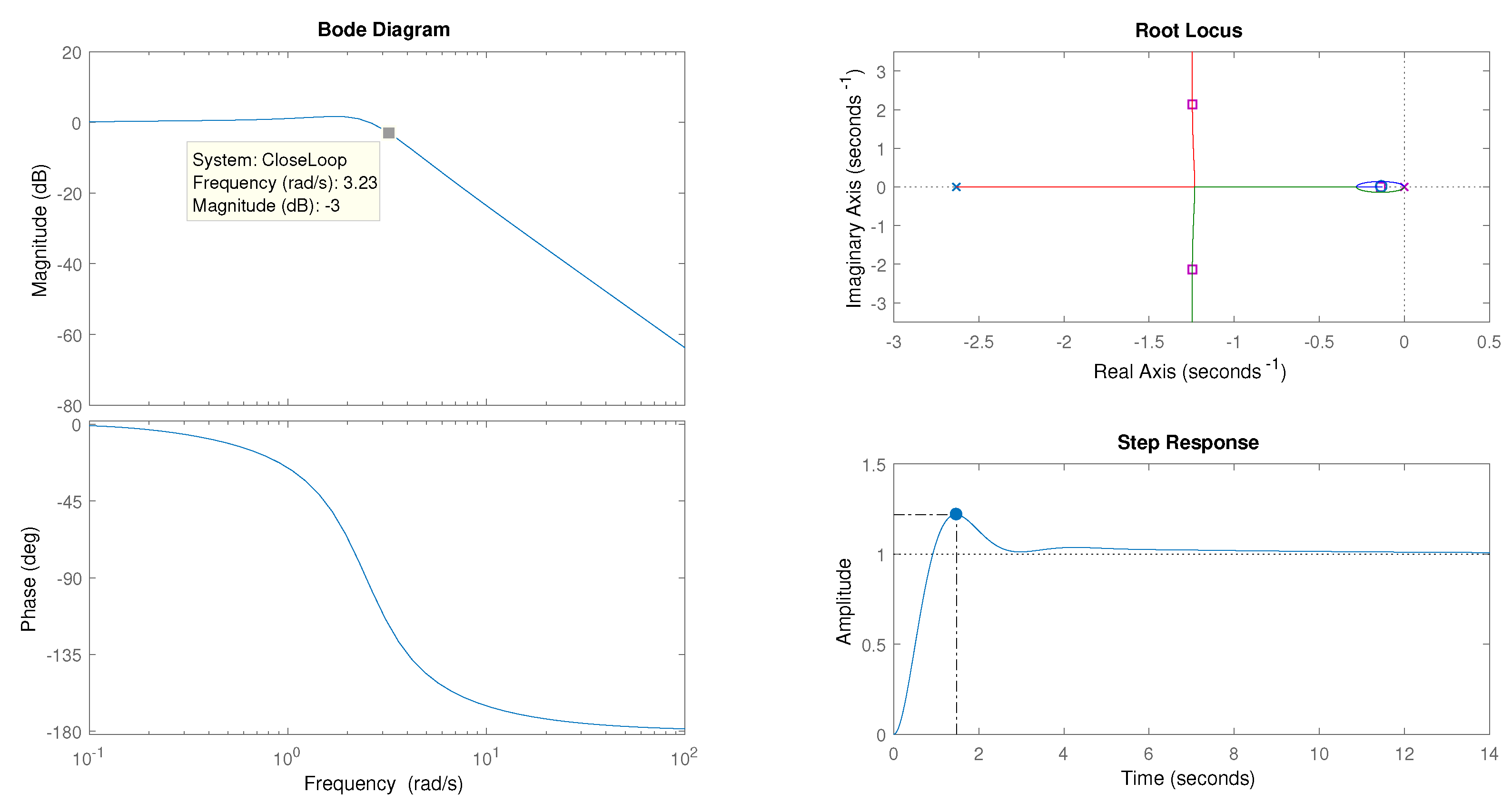Figure 8 presents the root locus, the step response, and the Bode diagram of the closed-loop system with the continuous time PI control.

Thus, in Figure 8 it is observed that the bandwidth of the closed-loop system is $w_{bw}=3.23$ rad/s. According to [35], the sample rate is usually taken between 10 and 20 times the bandwidth. For the design 20 times are taken; therefore, the sampling frequency is $w_s=20w_{bw}$ and thus the sampling time $T_s=2\pi /w_s$ is $T_s\approx 0.1s$.

The transfer function $G\left(s\right)$ given by Equation (14) is converted to $G\left(z\right)$ (discrete time system) using a sampling time of $T_s$ = 0.1 s and the bilinear transformation method [30]. In this way, the model of the discrete time system is obtained given by Equation (16).

$$G\left(z\right)={10}^{-5}\frac{2.907+5.814z^{-1}+2.907z^{-2}}{1-1.767z^{-1}+0.767z^{-2}}$$

(16)

In general, this transfer function can be represented as:

$$G\left(z\right)=\frac{\Theta \left(z\right)}{U\left(z\right)}=\frac{B_0+B_1{z}^{-1}+B_2^{-2}}{1+A_1{z}^{-1}+A_2{z}^{-2}}$$

(17)

The respective difference equation for this plant is:

$$\theta \left[n\right]=B_{0}u\left[n\right]+B_{1}u[n-1]+B_{2}u[n-2]-A_1\theta [n-1]-A_2\theta [n-2]$$

(18)

3. Fuzzy Control System

The neuro-fuzzy controller uses the structure of a compact fuzzy system based on Boolean relations such as that presented in [21], which can be used for the identification and control of dynamic systems. Fuzzy systems based on Boolean relations are based on a system design considering possible Boolean regions in the discourse universes; then this system is extended using fuzzy sets for implementation, making it possible to consider the operation of sensors and actuators present in the control system [22]. The output of these systems can be calculated as:

$$y=\sum _{i=1}^N{\nu }_i{Y}_i$$

(19)

where ${\nu }_i$ corresponds to the virtual actuator and $Y_i$ the activation output that depends on the membership functions ${\mu }_{l,j}\left(x_l\right)$ associated with inputs $x_l$ for $l=1,2,\dots ,L$ and $j=1,2,\dots ,M_l$.

In order to establish the activation functions $Y_i$, a truth table and various design considerations are used as well as the manipulation of the system equations using Boolean and Kleene algebras [22]. By using a compact structure, direct equivalence can be performed with the structure of a dynamic discrete time system, which allows the implementation of fuzzy controllers [21].

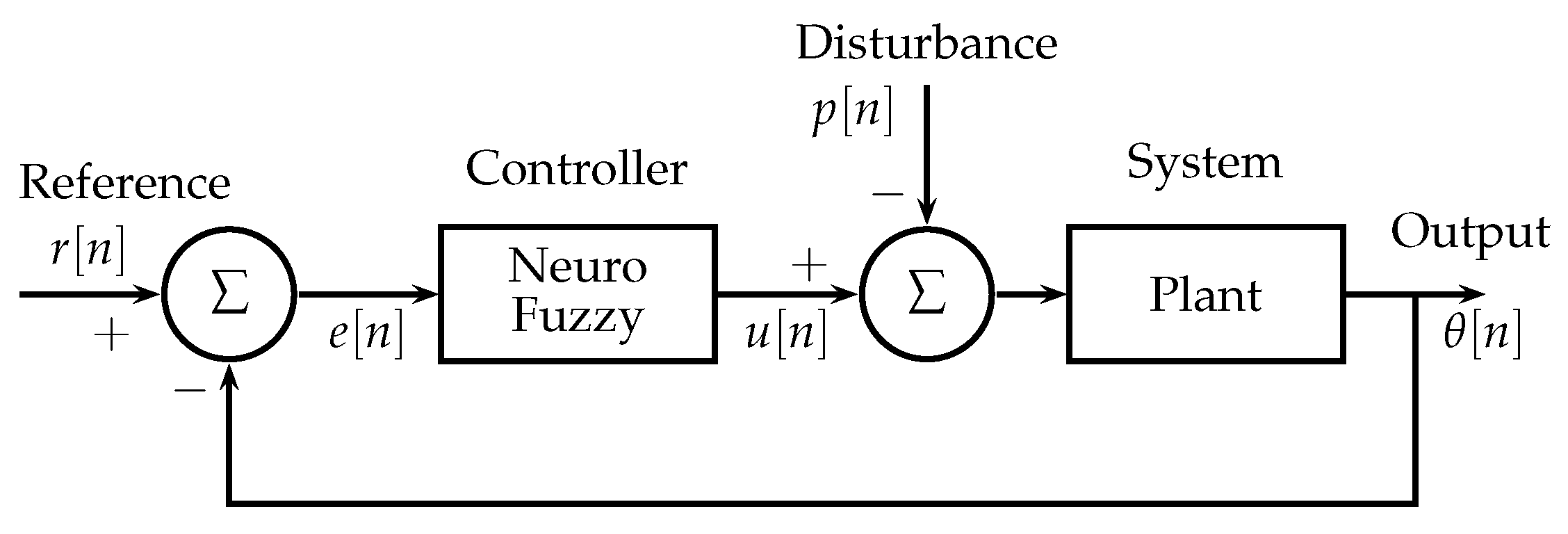
In this way, fuzzy control design consists of modifying (extending) a linear (discrete time) controller using fuzzy sets to model the controller non-linear relations. This design principle is used in [23] to control an automatic voltage regulator. The general diagram of the control system can be seen in Figure 9.

The fuzzy controller schema consists of modifying the non-linear relations that exist for the input and feedback signals. To carry out the design of the neuro-fuzzy controller, a linear PI (Proportional Integral) controller given by Equation (20) is considered.

$$C\left(s\right)=K_p+\frac{K_i}{s}=\frac{s{K}_p+K_i}{s}$$

(20)

Considering the controller in discrete time, the respective transfer function of the PI controller is:

$$C\left(z\right)=\frac{U\left(z\right)}{E\left(z\right)}=\frac{b_0-b_1{z}^{-1}}{1-z^{-1}}$$

(21)

The difference equation of this controller corresponds to:

$$u\left[n\right]=b_{0}e\left[n\right]-b_{1}e[n-1]+u[n-1]$$

(22)

where the respective coefficients $b_0$, $b_1$ are constant. For the fuzzy controller, these constants are replaced by non-linear relations given by fuzzy membership functions, such that:

$$u\left[n\right]=f_1\left(e\left[n\right]\right)-f_2\left(e[n-1]\right)+f_3\left(u[n-1]\right))$$

(23)

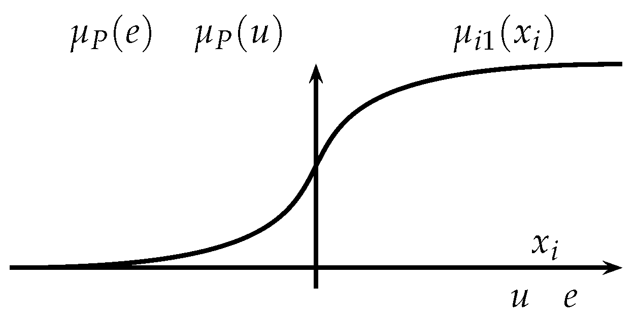
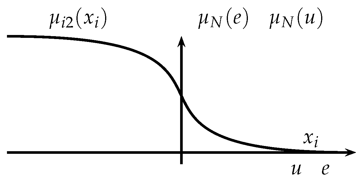
Fuzzy sets shown in Figure 10 and Figure 11 are employed for the fuzzy control system. Particularly, Figure 10 shows a sigmoidal fuzzy set to model positive values of the universe of discourse e and u, while in Figure 11 the negative values are represented for the error e and control action u.

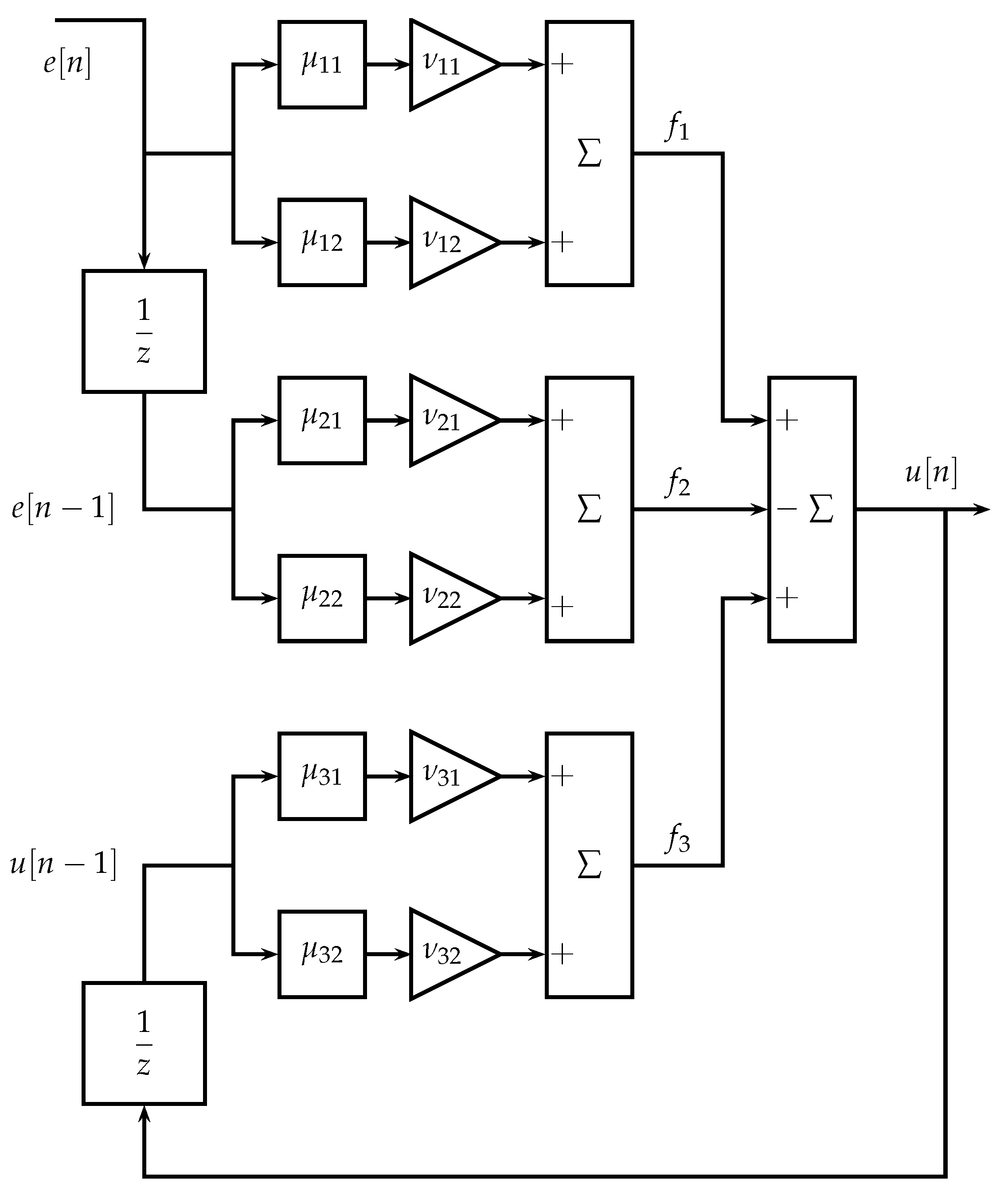
Considering the fuzzy sets described in Figure 10 and Figure 11, as well as the controller structure given by Equation (23), the scheme of Figure 12 is obtained, where the proposed fuzzy controller is shown.

The controller output can be calculated with Equation (24) where the inputs to the fuzzy system are $x_i\in \{e\left[n\right],e[n-1],u[n-1]\}$.

$$u\left[n\right]=\sum _{i=1}^3\sum _{j=1}^2{\nu }_{ij}{\mu }_{ij}\left(x_i\right)=\sum _{i=1}^3{f}_i\left(x_i\right)$$

(24)

For each input $x_i$ it is possible to define a function $f_i$ as presented in Equation (25).

$$f_i={\nu }_{i1}{\mu }_{i1}\left(x_i\right)+{\nu }_{i2}{\mu }_{i2}\left(x_i\right)$$

(25)

To carry out the respective calculations, the membership function is given by equation ${\mu }_{ij}\left(x_i\right)={(1+e^{-{\rho }_{ij}(x_i-{\chi }_{ij})})}^{-1}$; in this way, the set of controller parameters is ${\mathbf{H}}_c=\{{\nu }_{ij},{\rho }_{ij},{\chi }_{ij}\}$.

4. Controller Parameter Training

The structure of the closed-loop neuro-fuzzy controller can be assimilated as a recurrent neural network; according to [36], there are different alternatives to perform the training process. One way is to calculate the respective recurrent equation that updates each parameter using the respective fitness function derivatives. In this way, the system simulation will be carried out with the current parameters without modification; in the same simulation the adjustment of parameters is carried out in auxiliary variables, since these parameters are not used in the current simulation. When finishing the simulation, the system parameters are updated with those stored in the auxiliary variables and a new simulation is carried out until the value of the fitness function is reduced.

To carry out the controller training, first the structure of the plant and the controller are established; thus, for a closed-loop system, the control action corresponds to:

$$u\left[n\right]=f_c(e\left[n\right],e[n-1],u[n-1],{\mathbf{H}}_c)$$

(26)

Likewise, the system’s output employed for controller training is:

$$\theta \left[n\right]=f_p\left(u\left[n\right],u[n-1],\theta [n-1],\theta [n-2],{\mathbf{H}}_p\right)$$

(27)

where ${\mathbf{H}}_c$ corresponds to the set of controller parameters and ${\mathbf{H}}_p$ to the plant parameters. Considering $h_c$ as one of the control system parameters, the adaptation of the controller parameters is carried out using Equation (28).

$$h_c(k+1)=h_c\left(k\right)-\eta \frac{dJ}{d{h}_c}$$

(28)

In Equation (28), parameter $\eta$ is the learning rate and J corresponds to the adjustment function defined as:

$$J=\frac{1}{2}\left[Q{\left(e\left[n\right]\right)}^2+R{\left(u\left[n\right]\right)}^2\right]$$

(29)

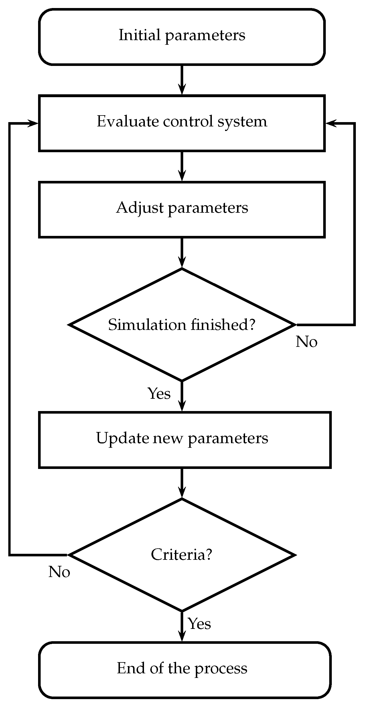
where $e\left[n\right]=r\left[n\right]-\theta \left[n\right]$ and the derivative of J depending on the adjustment parameters is given by Equation (30). Considering these equations, Figure 13 shows the algorithm employed for controller training.

$$\frac{dJ}{d{h}_c}=Qe\left[n\right]\frac{de}{d{h}_c}+Ru\left[n\right]\frac{du}{d{h}_c}$$

(30)

The first step consists of choosing the initial controller’s parameter configuration; then, the next step involves the system output calculation using the model of the plant. Subsequently, the parameter’s adjustment occurs employing the respective equations involved in the dynamics in the control system and the derivatives of the parameters (equations $de/d{h}_c$, $du/d{h}_c$ and subsequent). It is noteworthy that during the simulation the adjusted parameters are stored in auxiliary variables since during this process these values are not used by the controller. To continue the simulation and parameter adjustment, the algorithm returns to the step where the control system is evaluated with $n=n+1$, repeating this process until simulation time $N_T$ is complete. Once the simulation time is completed, the parameters of the controller are updated with the optimized values to return to the evaluation step of the control system to start a new iteration $k=k+1$ until the objective function $J_T\left(k\right)=(1/N_T){\sum }_{n=1}^{N_T}J(k,n)$ is less than a given $\epsilon$ or until k is equal to a given number $K_T$.

5. Equations for Linear Controller Parameter Training

The implementation of the training algorithm (dynamic back propagation) uses difference equations of each parameter in the adaptation Equation (28). On aspects to bear in mind in [37,38], the stability analysis is presented for this kind of algorithm used for training recurrent neural networks.

In order to determine the equations for linear controller training, first, the error equation is $e\left[n\right]=r\left[n\right]-\theta \left[n\right]$ where the output of the plant is given by Equation (31).

$$\theta \left[n\right]=B_{0}u\left[n\right]+B_{1}u[n-1]+B_{2}u[n-2]-A_1\theta [n-1]-A_2\theta [n-2]$$

(31)

Secondly, the difference equation of the controller is:

$$u\left[n\right]=b_{0}e\left[n\right]-b_{1}e[n-1]+u[n-1]$$

(32)

Therefore, the training equations of the parameters $h_c\in \{b_0,b_1\}$ are the following:

$$\frac{de}{d{h}_c}\left[n\right]=-\frac{d\theta }{d{h}_c}\left[n\right]$$

(33)

$$\frac{d\theta }{d{h}_c}\left[n\right]=B_0\frac{du}{d{h}_c}\left[n\right]+B_1\frac{du}{d{h}_c}[n-1]+B_2\frac{du}{d{h}_c}[n-2]-A_1\frac{d\theta }{d{h}_c}[n-1]-A_2\frac{d\theta }{d{h}_c}[n-2]$$

(34)

The derivative equation of $u\left[n\right]$ based on the controller parameter $b_0$ is:

$$\begin{array}{cc}\hfill \frac{du}{d{b}_0}\left[n\right]& =\frac{d}{d{b}_0}\left(b_{0}e\left[n\right]\right)-b_1\frac{de}{d{b}_0}[n-1]+\frac{du}{d{b}_0}[n-1]\hfill \\ \hfill & =b_0\frac{de}{d{b}_0}\left[n\right]-b_1\frac{de}{d{b}_0}[n-1]+\frac{du}{d{b}_0}[n-1]+e\left[n\right]\hfill \end{array}$$

(35)

Therefore, for the parameter $b_1$ the equation is:

$$\begin{array}{cc}\hfill \frac{du}{d{b}_1}\left[n\right]& =b_0\frac{de}{d{b}_1}\left[n\right]-\frac{d}{d{b}_1}\left(b_{1}e[n-1]\right)+\frac{du}{d{b}_1}[n-1]\hfill \\ \hfill & =b_0\frac{de}{d{b}_1}\left[n\right]-b_1\frac{de}{d{b}_1}[n-1]+\frac{du}{d{b}_1}[n-1]-e[n-1]\hfill \end{array}$$

(36)

In this way, using a learning rate $\eta$ the following equation is used to update the parameters:

$$h_c(k+1)=h_c\left(k\right)-\eta \left[Qe\left[n\right]\frac{de\left[n\right]}{d{h}_c}+Ru\left[n\right]\frac{du\left[n\right]}{d{h}_c}\right]$$

(37)

6. Equations for Fuzzy Controller Parameter Training

In this case, the training equations are established for the fuzzy controller based on Boolean relations; in this order, the equation of the plant is:

$$\theta \left[n\right]=B_{0}u\left[n\right]+B_{1}u[n-1]+B_{2}u[n-2]-A_1\theta [n-1]-A_2\theta [n-2]$$

(38)

Considering the controller architecture (Figure 12) and the expression for $f_i$ given by Equation (25), the controller dynamics is given by:

$$u\left[n\right]=f_1\left(e\left[n\right]\right)-f_2\left(e[n-1]\right)+f_3\left(u[n-1]\right)$$

(39)

Additionally,

$$e\left[n\right]=r\left[n\right]-\theta \left[n\right]$$

(40)

is used to calculate the error variable.

The respective derivative of the plant output $\theta \left[n\right]$ for a controller parameter $h_{ij}\in {\mathbf{H}}_c$ is:

$$\frac{d\theta }{d{h}_{ij}}\left[n\right]=B_0\frac{du}{d{h}_{ij}}\left[n\right]+B_1\frac{du}{d{h}_{ij}}[n-1]+B_2\frac{du}{d{h}_{ij}}[n-2]-A_1\frac{d\theta }{d{h}_{ij}}[n-1]-A_2\frac{d\theta }{d{h}_{ij}}[n-2]$$

(41)

In the same way, the derivative of the control action $u\left[n\right]$ with respect to $h_{ij}$ is:

$$\frac{du\left[n\right]}{d{h}_{ij}}=\frac{d{f}_1\left(e\left[n\right]\right)}{d{h}_{ij}}-\frac{d{f}_2\left(e[n-1]\right)}{d{h}_{ij}}+\frac{d{f}_3\left(u[n-1]\right)}{d{h}_{ij}}$$

(42)

Meanwhile, the derivative of the error $e\left[n\right]$ for a controller parameter $h_{ij}$ corresponds to:

$$\frac{de\left[n\right]}{d{h}_{ij}}=\frac{dr\left[n\right]}{d{h}_{ij}}-\frac{d\theta \left[n\right]}{d{h}_{ij}}=-\frac{d\theta \left[n\right]}{d{h}_{ij}}$$

(43)

To determine the respective derivatives, it is considered that:

$$\frac{d{f}_l\left(x_l\right)}{d{h}_{ij}}=\frac{d}{d{h}_{ij}}\left({\nu }_{l1}{\mu }_{l1}\left(x_l\right)\right)+\frac{d}{d{h}_{ij}}\left({\nu }_{l2}{\mu }_{l2}\left(x_l\right)\right)$$

(44)

where $l=1,\dots ,3$, $i=1,\dots ,3$ and $j=1,2$; therefore, there are different cases for values of i and l. According to the values of i, l and j the possible cases are:

• Case: $l\ne i$, where $f_l$ does not depend directly on $h_{ij}$.
• Case: $l=i$ and $j=1$, where $f_i$ directly depends on $h_{i1}$.
• Case: $l=i$ and $j=2$, where $f_i$ directly depends on $h_{i2}$.

In the case when $l\ne i$ it is obtained:

$$\frac{d{f}_l\left(x_l\right)}{d{h}_{ij}}=\frac{d}{d{x}_l}\left({\nu }_{l1}{\mu }_{l1}\left(x_l\right)\right)\frac{d{x}_l}{d{h}_{ij}}+\frac{d}{d{x}_l}\left({\nu }_{l2}{\mu }_{l2}\left(x_l\right)\right)\frac{d{x}_l}{d{h}_{ij}}$$

(45)

$$\frac{d{f}_l\left(x_l\right)}{d{h}_{ij}}=\left[\frac{d}{d{x}_l}\left({\nu }_{l1}{\mu }_{l1}\left(x_l\right)\right)+\frac{d}{d{x}_l}\left({\nu }_{l2}{\mu }_{l2}\left(x_l\right)\right)\right]\frac{d{x}_l}{d{h}_{ij}}$$

(46)

For $m=1,2$ the respective derivatives are:

$$\frac{d}{d{x}_l}\left({\nu }_{lm}{\mu }_{lm}\left(x_l\right)\right)=\frac{d}{d{x}_l}\left({\nu }_{lm}{\left(1+e^{-{\rho }_{lm}(x_l-{\chi }_{lm})}\right)}^{-1}\right)$$

(47)

$$\frac{d}{d{x}_l}\left({\nu }_{lm}{\mu }_{lm}\left(x_l\right)\right)=L_{lm}={\nu }_{lm}{\left(1+e^{-{\rho }_{lm}(x_l-{\chi }_{lm})}\right)}^{-2}{e}^{-{\rho }_{lm}(x_l-{\chi }_{lm})}{\rho }_{lm}$$

(48)

Meanwhile, when $l=i$ and $j=1$ it is established that:

$$\frac{d{f}_i\left(x_i\right)}{d{h}_{i1}}=\frac{d}{d{h}_{i1}}\left({\nu }_{i1}{\mu }_{i1}\left(x_i\right)\right)+\frac{d}{d{x}_i}\left({\nu }_{i2}{\mu }_{i2}\left(x_i\right)\right)\frac{d{x}_i}{d{h}_{i1}}$$

(49)

Now in the case where $l=i$ and $j=2$ it is presented that:

$$\frac{d{f}_i\left(x_i\right)}{d{h}_{i2}}=\frac{d}{d{x}_i}\left({\nu }_{i1}{\mu }_{i1}\left(x_i\right)\right)\frac{d{x}_i}{d{h}_{i2}}+\frac{d}{d{h}_{i2}}\left({\nu }_{i2}{\mu }_{i2}\left(x_i\right)\right)$$

(50)

In the first place, for the derivatives with respect to $x_i$ is obtained:

$$\frac{d}{d{x}_i}\left({\nu }_{ij}{\mu }_{ij}\left(x_i\right)\right)=L_{ij}={\nu }_{ij}{\left(1+e^{-{\rho }_{ij}(x_i-{\chi }_{ij})}\right)}^{-2}{e}^{-{\rho }_{ij}(x_i-{\chi }_{ij})}{\rho }_{ij}$$

(51)

Second, for the derivatives with respect to $h_{ij}$ it has:

$$\frac{d}{d{h}_{ij}}\left({\nu }_{ij}{\mu }_{ij}\left(x_i\right)\right)=\frac{d}{d{h}_{ij}}\left({\nu }_{ij}{\left(1+e^{-{\rho }_{ij}(x_i-{\chi }_{ij})}\right)}^{-1}\right)$$

(52)

In this way, for the respective parameters ${\nu }_{ij}$, ${\rho }_{ij}$ and ${\chi }_{ij}$ it is obtained that:

$$\begin{array}{cc}\hfill \frac{d}{d{\nu }_{ij}}\left({\nu }_{ij}{\mu }_{ij}\left(x_i\right)\right)& ={\left(1+e^{-{\rho }_{ij}(x_i-{\chi }_{ij})}\right)}^{-1}+{\nu }_{ij}{\left(1+e^{-{\rho }_{ij}(x_i-{\chi }_{ij})}\right)}^{-2}{e}^{-{\rho }_{ij}(x_i-{\chi }_{ij})}{\rho }_{ij}\frac{d{x}_i}{d{\nu }_{ij}}\hfill \end{array}$$

(53)

$$\begin{array}{cc}\hfill \frac{d}{d{\rho }_{ij}}\left({\nu }_{ij}{\mu }_{ij}\left(x_i\right)\right)& =-{\nu }_{ij}{\left(1+e^{-{\rho }_{ij}(x_i-{\chi }_{ij})}\right)}^{-2}{e}^{-{\rho }_{ij}(x_i-{\chi }_{ij})}\left({\chi }_{ij}-x_i-{\rho }_{ij}\frac{d{x}_i}{d{\rho }_{ij}}\right)\hfill \end{array}$$

(54)

$$\begin{array}{cc}\hfill \frac{d}{d{\chi }_{ij}}\left({\nu }_{ij}{\mu }_{ij}\left(x_i\right)\right)& =-{\nu }_{ij}{\left(1+e^{-{\rho }_{ij}(x_i-{\chi }_{ij})}\right)}^{-2}{e}^{-{\rho }_{ij}(x_i-{\chi }_{ij})}\left({\rho }_{ij}-{\rho }_{ij}\frac{d{x}_i}{d{\chi }_{ij}}\right)\hfill \end{array}$$

(55)

In general terms for $h_{ij}$ these equations can be written as:

$$\frac{d}{d{h}_{ij}}\left({\nu }_{ij}{\mu }_{ij}\left(x_i\right)\right)=T_{h_{ij}}+C_{ij}\frac{d{x}_i}{d{h}_{ij}}$$

(56)

Considering the parameters ${\nu }_{ij}$, ${\rho }_{ij}$ and ${\chi }_{ij}$ it has:

$$\frac{d}{d{\nu }_{ij}}\left({\nu }_{ij}{\mu }_{ij}\left(x_i\right)\right)=T_{{\nu }_{ij}}+C_{ij}\frac{d{x}_i}{d{\nu }_{ij}}$$

(57)

$$\frac{d}{d{\rho }_{ij}}\left({\nu }_{ij}{\mu }_{ij}\left(x_i\right)\right)=T_{{\rho }_{ij}}+C_{ij}\frac{d{x}_i}{d{\rho }_{ij}}$$

(58)

$$\frac{d}{d{\chi }_{ij}}\left({\nu }_{ij}{\mu }_{ij}\left(x_i\right)\right)=T_{{\chi }_{ij}}+C_{ij}\frac{d{x}_i}{d{\chi }_{ij}}$$

(59)

where:

$$\begin{array}{cc}\hfill C_{ij}& ={\nu }_{ij}{\left(1+e^{-{\rho }_{ij}(x_i-{\chi }_{ij})}\right)}^{-2}{e}^{-{\rho }_{ij}(x_i-{\chi }_{ij})}{\rho }_{ij}\hfill \end{array}$$

(60)

$$\begin{array}{cc}\hfill T_{{\nu }_{ij}}& ={\left(1+e^{-{\rho }_{ij}(x_i-{\chi }_{ij})}\right)}^{-1}\hfill \end{array}$$

(61)

$$\begin{array}{cc}\hfill T_{{\rho }_{ij}}& =-{\nu }_{ij}{\left(1+e^{-{\rho }_{ij}(x_i-{\chi }_{ij})}\right)}^{-2}{e}^{-{\rho }_{ij}(x_i-{\chi }_{ij})}\left({\chi }_{ij}-x_i\right)\hfill \end{array}$$

(62)

$$\begin{array}{cc}\hfill T_{{\chi }_{ij}}& =-{\nu }_{ij}{\left(1+e^{-{\rho }_{ij}(x_i-{\chi }_{ij})}\right)}^{-2}{e}^{-{\rho }_{ij}(x_i-{\chi }_{ij})}{\rho }_{ij}\hfill \end{array}$$

(63)

Considering the above for the Equation (46) (case $l\ne i$), it can be written in the form:

$$\begin{array}{cc}\hfill \frac{d{f}_l\left(x_l\right)}{d{h}_{ij}}& =\left[\frac{d}{d{x}_l}\left({\nu }_{l1}{\mu }_{l1}\left(x_l\right)\right)+\frac{d}{d{x}_l}\left({\nu }_{l2}{\mu }_{l2}\left(x_l\right)\right)\right]\frac{d{x}_l}{d{h}_{ij}}\hfill \\ \hfill & =\left[L_{l1}+L_{l2}\right]\frac{d{x}_l}{d{h}_{ij}}\hfill \end{array}$$

(64)

On the other hand, for Equation (49) (case $l=i$, $j=1$) the following representation is stated:

$$\begin{array}{cc}\hfill \frac{d{f}_i\left(x_i\right)}{d{h}_{i1}}& =\frac{d}{d{h}_{i1}}\left({\nu }_{l1}{\mu }_{i1}\left(x_i\right)\right)+\frac{d}{d{x}_i}\left({\nu }_{i2}{\mu }_{i2}\left(x_i\right)\right)\frac{d{x}_i}{d{h}_{i1}}\hfill \\ \hfill & =T_{h_{i1}}+C_{i1}\frac{d{x}_i}{d{h}_{i1}}+L_{i2}\frac{d{x}_i}{d{h}_{i1}}\hfill \\ \hfill & =T_{h_{i1}}+\left[C_{i1}+L_{i2}\right]\frac{d{x}_i}{d{h}_{i1}}\hfill \end{array}$$

(65)

Meanwhile for the Equation (50) (case $l=i$, $j=2$) it is obtained:

$$\begin{array}{cc}\hfill \frac{d{f}_i\left(x_i\right)}{d{h}_{i2}}& =\frac{d}{d{x}_i}\left({\nu }_{l1}{\mu }_{i1}\left(x_i\right)\right)\frac{d{x}_i}{d{h}_{i2}}+\frac{d}{d{h}_{i2}}\left({\nu }_{i2}{\mu }_{i2}\left(x_i\right)\right)\hfill \\ \hfill & =L_{i1}\frac{d{x}_i}{d{h}_{i2}}+T_{h_{i2}}+C_{i2}\frac{d{x}_i}{d{h}_{i2}}\hfill \\ \hfill & =T_{h_{i2}}+\left[L_{i1}+C_{i2}\right]\frac{d{x}_i}{d{h}_{i2}}\hfill \end{array}$$

(66)

Finally, Equations (67)–(69) are employed to update the parameters, here $\eta$ corresponds to the learning rate.

$${\nu }_{ij}(k+1)={\nu }_{ij}\left(k\right)-\eta \left[Qe\left[n\right]\frac{de\left[n\right]}{d{\nu }_{ij}}+Ru\left[n\right]\frac{du\left[n\right]}{d{\nu }_{ij}}\right]$$

(67)

$${\rho }_{ij}(k+1)={\rho }_{ij}\left(k\right)-\eta \left[Qe\left[n\right]\frac{de\left[n\right]}{d{\rho }_{ij}}+Ru\left[n\right]\frac{du\left[n\right]}{d{\rho }_{ij}}\right]$$

(68)

$${\chi }_{ij}(k+1)={\chi }_{ij}\left(k\right)-\eta \left[Qe\left[n\right]\frac{de\left[n\right]}{d{\chi }_{ij}}+Ru\left[n\right]\frac{du\left[n\right]}{d{\chi }_{ij}}\right]$$

(69)

7. Results

Using the equations described in Section 5 and Section 6, the respective optimization of the control system is carried out for both the linear and fuzzy controllers. The settings for the Q and R values are as follows:

• QR1: $Q=1$, $R=0.00005$.
• QR2: $Q=1$, $R=0.0001$.
• QR3: $Q=1$, $R=0.0005$.
• QR4: $Q=1$, $R=0.001$.

After the training process Figure 14 shows the results when considering different reference values using the PI discrete linear controller.

The transfer functions of the PI controller obtained to Q and R values are the following:

• QR1:

  $$C\left(z\right)=\frac{66.79z-66.67}{z-1}=\frac{66.79(z-0.9982)}{(z-1)}$$
• QR2:

  $$C\left(z\right)=\frac{48.48z-48.39}{z-1}=\frac{48.48(z-0.9981)}{(z-1)}$$
• QR3:

  $$C\left(z\right)=\frac{22.66z-22.62}{z-1}=\frac{22.66(z-0.9982)}{(z-1)}$$
• QR4:

  $$C\left(z\right)=\frac{16.11z-16.08}{z-1}=\frac{16.11(z-0.9981)}{(z-1)}$$

The stability analysis for linear controller consists of determining the closed-loop poles of the control system (controller and plant). In this order, if the poles are in the unit circle the system is stable. For each case the transfer function $T\left(z\right)$ in a closed loop is:

• QR1:

  $$T\left(z\right)=\frac{0.001942z^3+0.001945z^2-0.001935z-0.001938}{1.002z^3-2.765z^2+2.532z-0.7689}$$
• QR2:

  $$T\left(z\right)=\frac{0.001409z^3+0.001412z^2-0.001404z-0.001407}{1.001z^3-2.766z^2+2.533z-0.7684}$$
• QR3:

  $$T\left(z\right)=\frac{0.0006587z^3+0.0006599z^2-0.0006564z-0.0006576}{1.001z^3-2.766z^2+2.533z-0.7677}$$
• QR4:

  $$T\left(z\right)=\frac{0.0004683z^3+0.0004692z^2-0.0004666z-0.0004674}{z^3-2.767z^2+2.534z-0.7675}$$

The respective pole localization is presented in

Table 1. Pole localization for each QR case.

QR1	QR2	QR3	QR4
0.9981	0.9980	0.9978	0.9971
0.9639	0.9756	0.9905	0.9947
0.7978	0.7881	0.7762	0.7734

. It is observed that the poles are within the unit circle. Therefore, all the systems in a closed loop are stable.

Additionally, as observed, the controllers display the zero near to $z=0.998$, while the gain K has the values $66.79$, $48.48$, $22.66$ and $16.11$. Moreover, when incrementing the value of R (which weighs the action control), the gain value of the K controller is reduced. Furthermore, it is seen that the algorithm establishes the zero near the pole, therefore the pole and zero “almost cancel” which is consistent with reference [34] for the PI controller design.

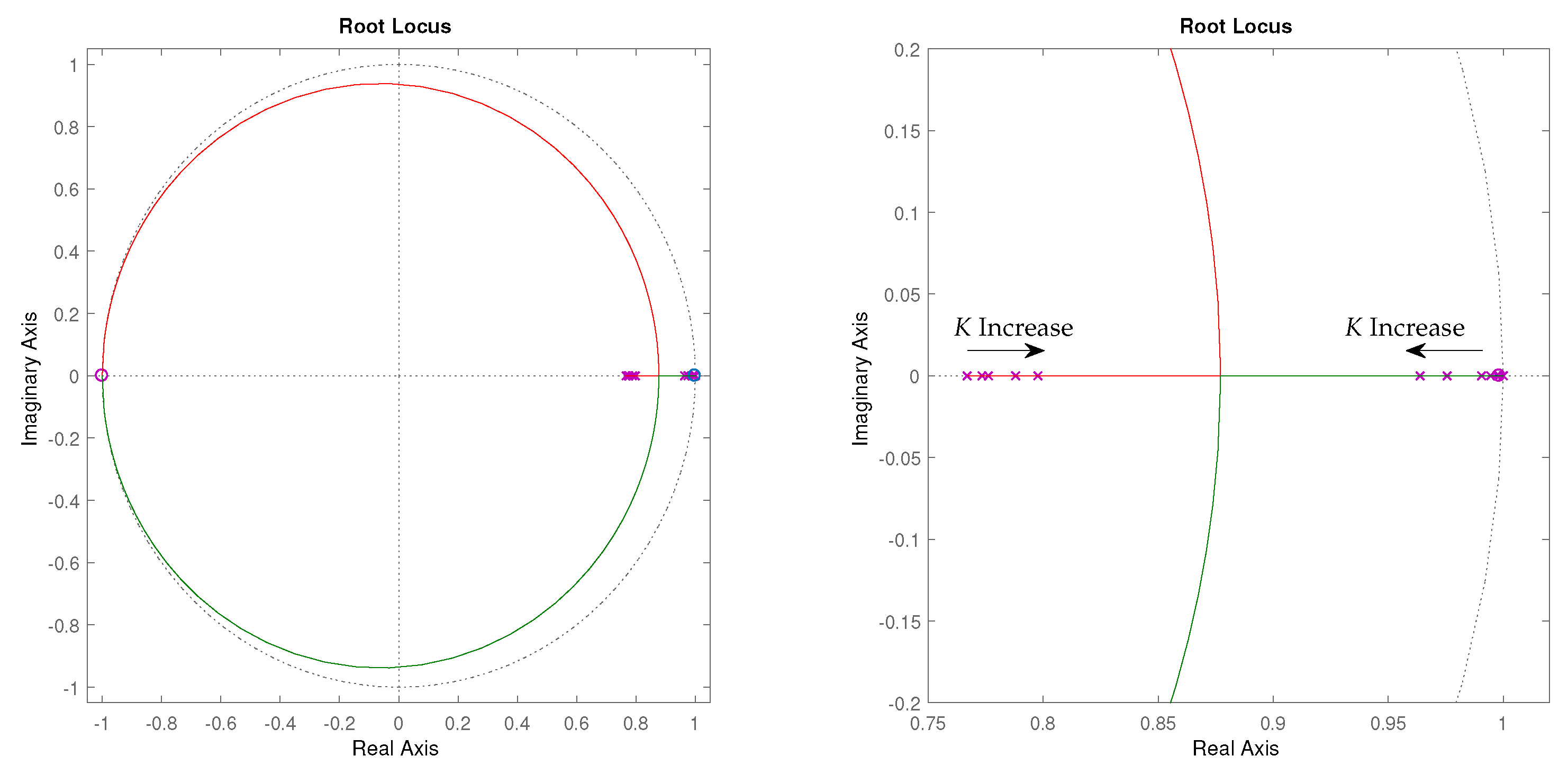
As results analysis, Figure 15 shows the root locus for the PI control system. This figure also displays the movement of the roots as the gain K increases.

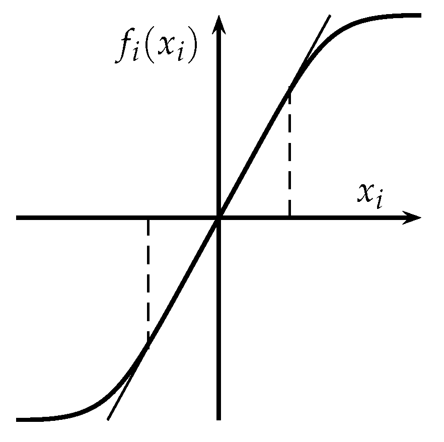
Employing configurations of functions $f_i\left(x_i\right)$ shown in Figure 16, it is possible to use the values obtained from the optimization of the linear controller to define an initial configuration to optimize the fuzzy controller. Thus, the slope of $f_i$ in the linear region is set to be equivalent with each parameter of the linear controller.

The fuzzy controller parameters obtained, with which the simulation of the closed-loop system can be performed, are shown in

Table 2. Fuzzy controller parameters for QR cases.

Fuzzy controller parameters for QR1 case
${\nu }_{ij}$			${\rho }_{ij}$	${\chi }_{ij}$
$-1.3358\times {10}^4$	$1.3358\times {10}^4$	$-0.0101$	$0.0101$	$-0.3382\times {10}^{-5}$	$-0.3382\times {10}^{-5}$
$1.3334\times {10}^4$	$-1.3334\times {10}^4$	$-0.0099$	$0.0099$	$0.3446\times {10}^{-5}$	$0.3446\times {10}^{-5}$
$-0.0200\times {10}^4$	$0.0200\times {10}^4$	$-0.0100$	$0.0100$	0	0
Fuzzy controller parameters for QR2 case
${\nu }_{ij}$		${\rho }_{ij}$		${\chi }_{ij}$
$-9.6960\times {10}^3$	$9.6960\times {10}^3$	$-0.0100$	$0.0100$	$-0.1066\times {10}^{-5}$	$-0.1066\times {10}^{-5}$
$9.6780\times {10}^3$	$-9.6780\times {10}^3$	$-0.0100$	$0.0100$	$0.1064\times {10}^{-5}$	$0.1064\times {10}^{-5}$
$-0.2000\times {10}^3$	$0.2000\times {10}^3$	$-0.0100$	$0.0100$	0	0
Fuzzy controller parameters for QR3 case
${\nu }_{ij}$		${\rho }_{ij}$		${\chi }_{ij}$
$-4.5320\times {10}^3$	$4.5320\times {10}^3$	$-0.0100$	$0.0100$	$0.1086\times {10}^{-6}$	$0.1086\times {10}^{-6}$
$4.5240\times {10}^3$	$-4.5240\times {10}^3$	$-0.0100$	$0.0100$	$-0.1081\times {10}^{-6}$	$-0.1081\times {10}^{-6}$
$-0.2000\times {10}^3$	$0.2000\times {10}^3$	$-0.0100$	$0.0100$	0	0
Fuzzy controller parameters for QR4 case
${\nu }_{ij}$		${\rho }_{ij}$		${\chi }_{ij}$
$-3.2220\times {10}^3$	$3.2220\times {10}^3$	$-0.0100$	$0.0100$	$0.6994\times {10}^{-7}$	$0.6994\times {10}^{-7}$
$3.2160\times {10}^3$	$-3.2160\times {10}^3$	$-0.0100$	$0.0100$	$-0.6982\times {10}^{-7}$	$-0.6982\times {10}^{-7}$
$-0.2000\times {10}^3$	$0.2000\times {10}^3$	$-0.0100$	$0.0100$	0	0

. As can be seen, there are different parameters considering the QR case. In this table, i corresponds to rows and j to columns.

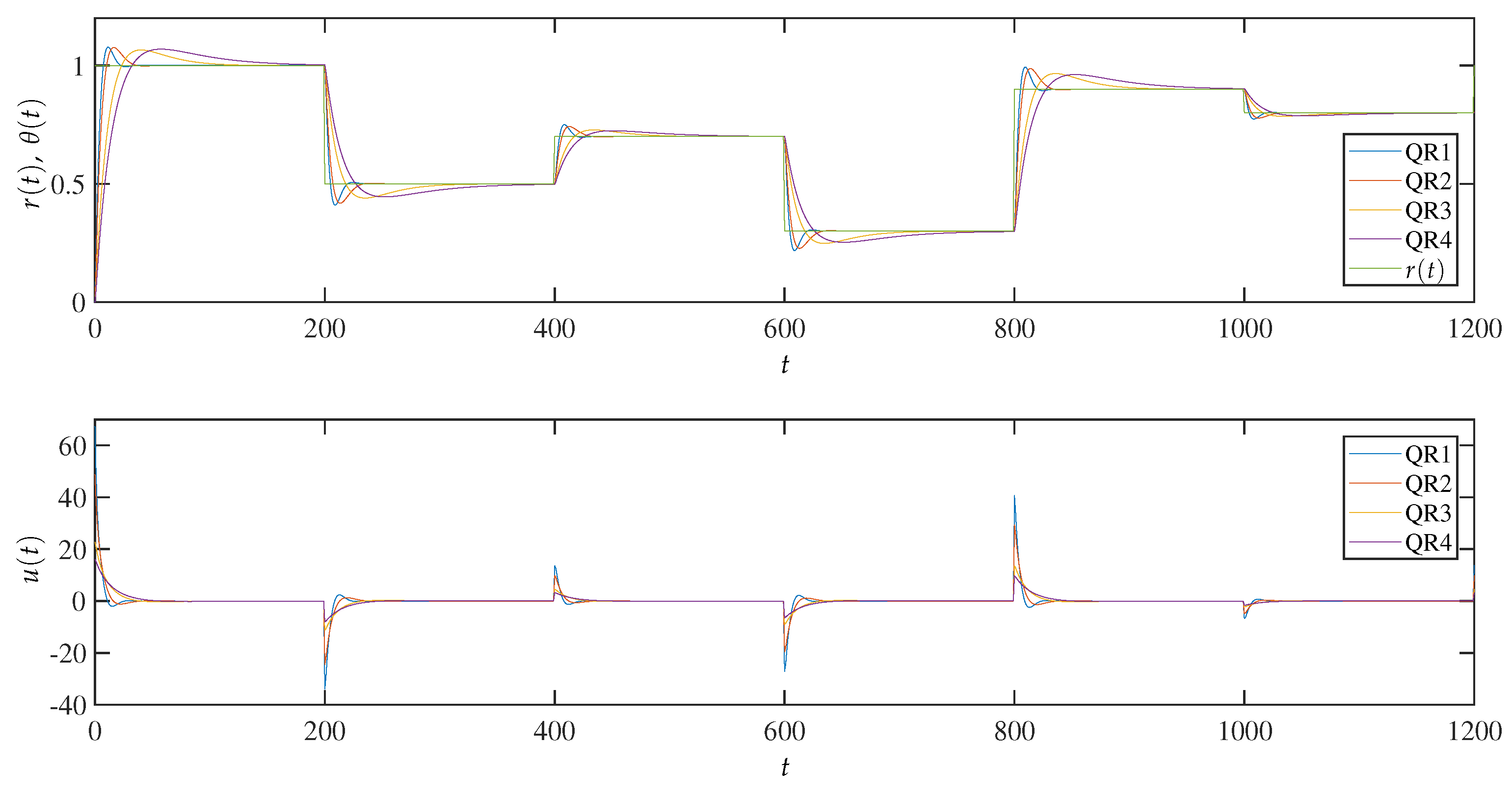
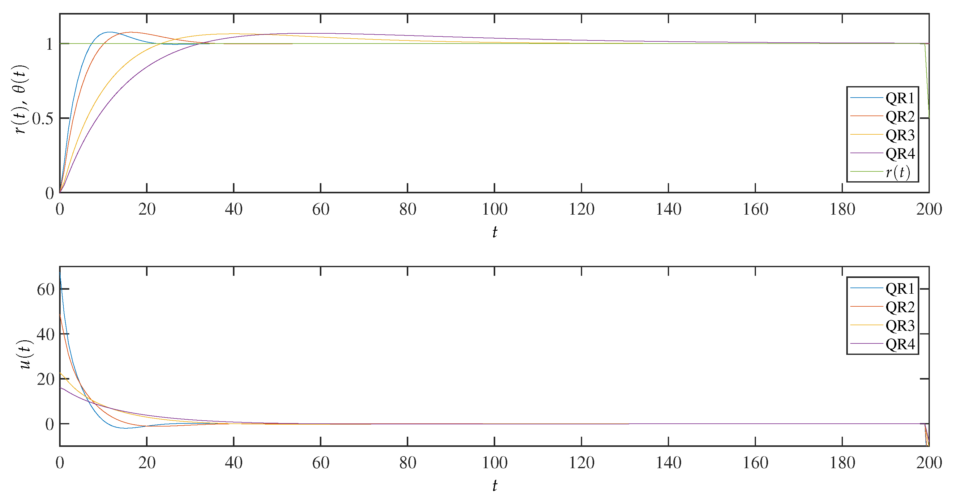
After performing the fuzzy controller training, Figure 17 shows the system response for different reference values, as well as the value of the control signal; additionally, Figure 18 shows in detail the system response for a unitary reference. According to simulations, the suitable configurations correspond to QR2 or QR3 considering the values of control action and settling time.

On the other hand,

Table 3. Initial and final values for $J_T$ in each configuration.

QR	Linear		Fuzzy
Case	Initial	Final	Initial	Final
QR1	0.0240293	0.0077754	0.0082463	0.0077858
QR2	0.0301406	0.0101258	0.0103760	0.0101451
QR3	0.1424850	0.0197969	0.0198750	0.0198434
QR4	0.4415530	0.0269572	0.0270372	0.0270370

presents the values obtained for $J_T$ in the initial and the final iteration (30 iterations) when performing the optimization process. These results show that the value of the objective function $J_T$ increases when increasing the value of R.

In addition, Table 3 shows that linear and fuzzy controls obtain similar values of $J_T$. These results highlight that the design and choice of the initial configuration of the fuzzy controller were satisfactory since it presents a similar result to the linear controller.

To statistically observe the performance of the linear and fuzzy controllers for different values of Q and R 10 simulations were performed with randomly generated $r\left(t\right)$ reference values (six variations in each simulation). Results of $J_T$ for 10 simulations are shown in

Table 4. Results of $J_T$ for 10 simulations.

Simulation	QR1		QR2		QR3		QR4
Run	Linear	Fuzzy	Linear	Fuzzy	Linear	Fuzzy	Linear	Fuzzy
1	0.0032	0.0033	0.0044	0.0044	0.0092	0.0090	0.0130	0.0126
2	0.0018	0.0019	0.0024	0.0025	0.0051	0.0050	0.0071	0.0069
3	0.0043	0.0044	0.0058	0.0058	0.0122	0.0119	0.0172	0.0166
4	0.0032	0.0032	0.0043	0.0043	0.0090	0.0088	0.0127	0.0123
5	0.0046	0.0046	0.0062	0.0062	0.0130	0.0127	0.0184	0.0178
6	0.0017	0.0018	0.0023	0.0023	0.0048	0.0047	0.0067	0.0066
7	0.0018	0.0018	0.0024	0.0025	0.0051	0.0051	0.0073	0.0070
8	0.0009	0.0010	0.0013	0.0013	0.0026	0.0026	0.0037	0.0036
9	0.0009	0.0010	0.0012	0.0013	0.0026	0.0026	0.0037	0.0036
10	0.0025	0.0026	0.0034	0.0034	0.0069	0.0068	0.0097	0.0094

, while

Table 5. Numerical measures of $J_T$ for 10 simulations.

Numerical	QR1		QR2		QR3		QR4
Measure	Linear	Fuzzy	Linear	Fuzzy	Linear	Fuzzy	Linear	Fuzzy
Mean	0.0025	0.0026	0.0034	0.0034	0.0070	0.0069	0.0099	0.0096
STD	0.0013	0.0013	0.0017	0.0017	0.0037	0.0036	0.0052	0.0050
Max	0.0046	0.0046	0.0062	0.0062	0.0130	0.0127	0.0184	0.0178
Min	0.0009	0.0010	0.0012	0.0013	0.0026	0.0026	0.0037	0.0036

displays the mean, Standard Deviation (STD), maximum and minimum values.

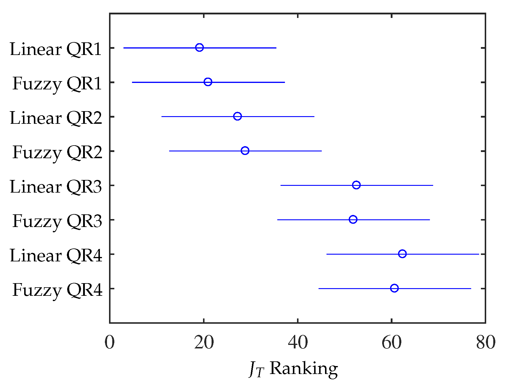
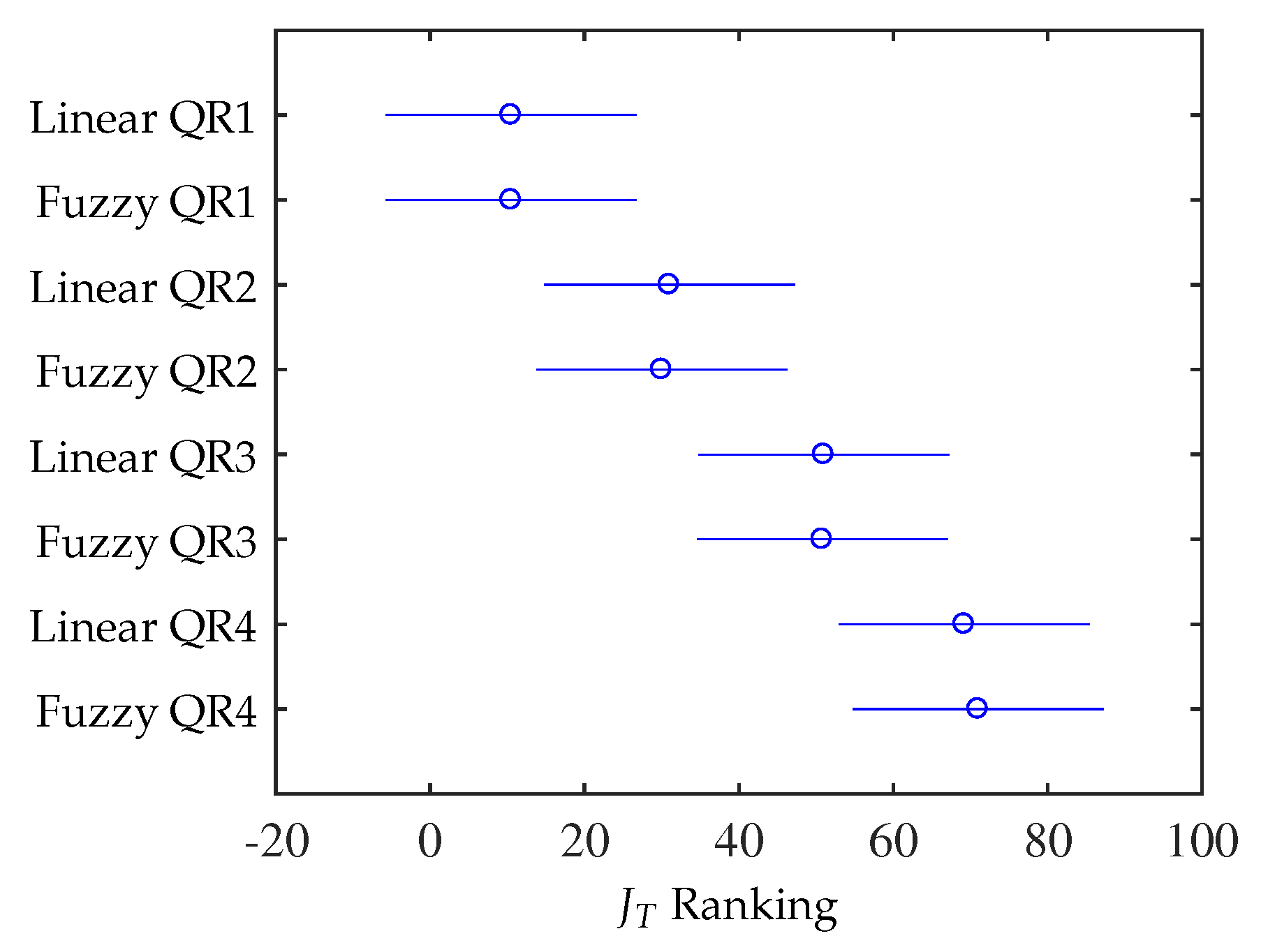
Regarding the statistical tests application [39], the Kruskal–Wallis test is used to determine statistically significant differences between two or more experimental groups, obtaining a p value of $3.7814\times {10}^{-7}$, which indicates differences, then it the Bonferroni procedure is employed to perform multiple comparisons, the results are presented in Figure 19, where we observe no significant difference between the linear and fuzzy implementations for the Q and R configurations. We also observed a significant difference between cases QR1 and QR4.

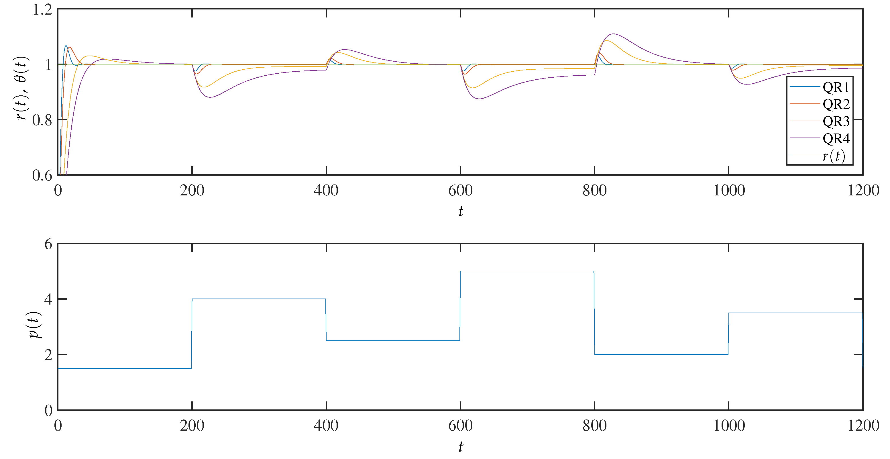
Meanwhile, Figure 20 shows the system behavior for $\theta \left(t\right)$ when there are disturbances $p\left(t\right)$. This figure also displays the responses for different configurations in Q and R. It can be observed that the disturbance effect is more noticeable for the controllers that employ a small signal control, as in the cases QR3 and QR4 (according to Figure 17 and Figure 18).

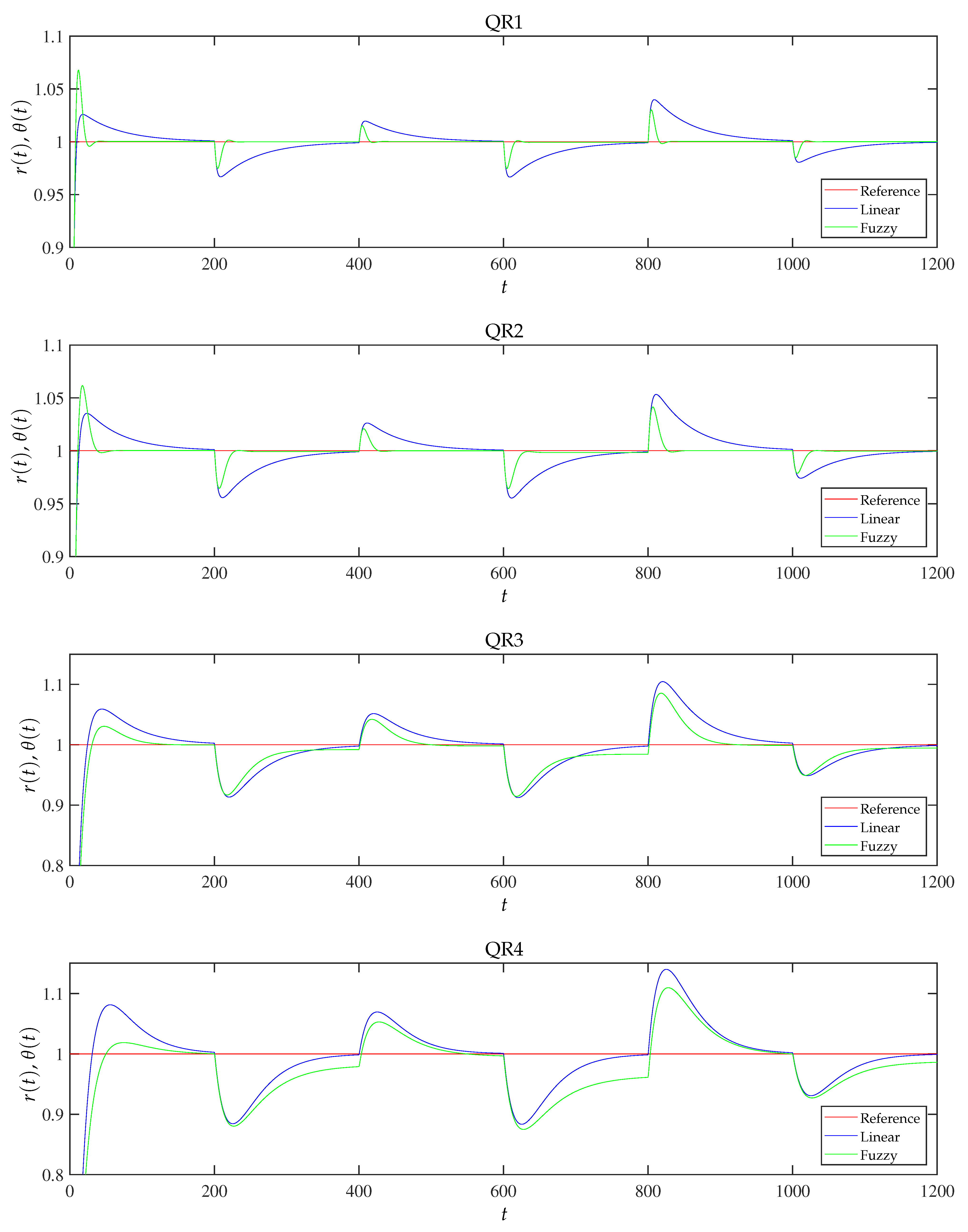
In Figure 21, the behavior comparison of the linear and fuzzy controllers is presented considering different perturbation values. For the disturbance values considered (Figure 18), some fuzzy controller configurations decrease the disturbance rejection capacity.

In order to statistically observe the performance of the linear and fuzzy controllers for disturbance rejection (considering different values of Q and R) 10 simulations were performed with randomly generated $p\left(t\right)$ disturbance values (six variations in each simulation). Results of $J_T$ for 10 simulations are shown in

Table 6. Disturbance rejection results of $J_T$ for 10 simulations.

Simulation	QR1		QR2		QR3		QR4
Run	Linear	Fuzzy	Linear	Fuzzy	Linear	Fuzzy	Linear	Fuzzy
1	0.0025	0.0024	0.0038	0.0036	0.0119	0.0116	0.0208	0.0213
2	0.0024	0.0024	0.0036	0.0035	0.0109	0.0107	0.0189	0.0190
3	0.0023	0.0023	0.0034	0.0033	0.0101	0.0100	0.0172	0.0178
4	0.0027	0.0028	0.0043	0.0044	0.0147	0.0153	0.0264	0.0289
5	0.0023	0.0023	0.0034	0.0034	0.0103	0.0102	0.0176	0.0180
6	0.0023	0.0023	0.0034	0.0033	0.0099	0.0099	0.0168	0.0178
7	0.0020	0.0020	0.0029	0.0028	0.0075	0.0072	0.0120	0.0120
8	0.0024	0.0024	0.0036	0.0036	0.0111	0.0114	0.0192	0.0205
9	0.0022	0.0022	0.0031	0.0031	0.0088	0.0086	0.0145	0.0147
10	0.0022	0.0022	0.0032	0.0031	0.0090	0.0090	0.0149	0.0157

, in this way,

Table 7. Numerical measures of $J_T$ for 10 simulations considering disturbance rejection.

Numerical	QR1		QR2		QR3		QR4
Measure	Linear	Fuzzy	Linear	Fuzzy	Linear	Fuzzy	Linear	Fuzzy
Mean	0.0023	0.0023	0.0035	0.0034	0.0104	0.0104	0.0178	0.0186
STD	0.0002	0.0002	0.0004	0.0004	0.0020	0.0022	0.0039	0.0045
Max	0.0027	0.0028	0.0043	0.0044	0.0147	0.0153	0.0264	0.0289
Min	0.0020	0.0020	0.0029	0.0028	0.0075	0.0072	0.0120	0.0120

displays the mean, standard deviation, and maximum and minimum values.

Considering Table 6 and Table 7, to determine statistically significant differences among the groups, we used the Kruskal–Wallis test, having a p-value of $2.8463\times {10}^{-13}$, which indicates differences. Considering the above result, the multiple comparisons using Bonferroni procedure is performed, obtaining Figure 22 observing no significant difference between the linear and fuzzy controllers for the configurations of Q and R. In addition, Figure 22 allows us to observe differences among cases QR1, QR2, QR3, and QR4, for example, when the value of R is increased the value of $J_T$ also increases.

8. Discussion

As seen, for linear controller the algorithm locates the zero near the pole in such a way that the pole and zero “almost cancel” occurs, which is a PI controller design method as presented in [34]. Frequently, it is possible to create a design by placing the zero of the controllers near the pole of origin in a way that both pole and zero of the system in closed loop “almost cancel” each other. Considering [33,34], a pair pole-zero that almost cancels has an insignificant effect on the time response; thus, the transitory response of the closed-loop system with the controller is approximately the same as in the closed-loop system without the controller. As a result, PI controller offers little deterioration in the transitory response with a significant improvement in steady state error.

According to [40], a prefilter can be employed to improve the system’s dynamic response. In the linear controller, the prefilter allows the cancellation of the zero effect; also, the system overshoot can be reduced with an adequate prefilter design. The effect of the prefilter might be included in the training algorithm for the optimization of the neuro-fuzzy system. The prefilter may have a linear design and then extend it to a fuzzy design.

This application shows the possibility of achieving a non-linear fuzzy controller taking as reference the design of a linear controller (linear controllers with excellent performance can be used for the plant). As the plant considered is well known, the article focuses on showing how a linear controller can be extended to a fuzzy controller (starting from a behavior close to the linear controller). After having the first implementation for the fuzzy controller, nonlinearities can be included to improve the behavior of the control system when having more complex plants with nonlinearities, a subject that will be addressed in later work. In addition, it can be considered a broader comparison with other techniques using different plants.

Further, in this work, the stability analysis of the closed-loop system was performed with the linear controller, in a later work it is expected to extend the stability analysis for this type of fuzzy controllers by means of a Liapunov analysis.

9. Conclusions

Linear controller design and optimization allow the design of the fuzzy controller as well as the definition of the initial optimization setup of this controller.

For the linear controller (in discrete time), since the pole of the controller is placed in $z=1$, the employed algorithm aims at finding the optimal location for the zero. Then, the fuzzy controller is optimized by considering these values for the initial setup; therefore, similar behavior is obtained. This demonstrates that it is possible to carry out the design and optimization of the fuzzy controller having a linear controller as a reference.

The fuzzy controller permits to include nonlinear relations through membership functions. Adequate configurations of these functions also allow the definition of a linear region in a way that it is possible to determine equivalence between the linear and fuzzy controllers.

The use of values Q and R permits obtaining different behaviors considering the action values that may be supplied for the plant. When testing the fuzzy controller for different reference values, the behavior of the control system is similar for the considered reference values.

It is observed that keeping the value of Q constant and increasing the value of R, the gain of the controller is reduced in a way that the energy of the plant also decreases.

The fuzzy controller scheme can be used for the implementation of an adaptive control strategy, in such a way that when a variation of the plant parameters occurs, the controller can be adjusted to obtain the desired behavior.