Comparison of Machine Learning Algorithms Used for Skin Cancer Diagnosis

Abstract

The paper presents a comparison of automatic skin cancer diagnosis algorithms based on analyses of skin lesions photos. Two approaches are presented: the first one is based on the extraction of features from images using simple feature descriptors, and then the use of selected machine learning algorithms for the purpose of classification, and the second approach uses selected algorithms belonging to the subgroup of machine learning—deep learning, i.e., convolutional neural networks (CNN), which perform both the feature extraction and classification in one algorithm. The following algorithms were analyzed and compared: Logistic Regression, k-Nearest Neighbors, Naive Bayes, Decision Tree, Random Forest, and Support Vector Machine, and four CNN–VGG-16, ResNet60, InceptionV3, and Inception-ResNetV2 In the first variant, before the classification process, the image features were extracted using 4 different feature descriptors and combined in various combinations in order to obtain the most accurate image features vector, and thus the highest classification accuracy. The presented approaches have been validated using the image dataset from the ISIC database, which includes data from two categories—benign and malignant skin lesions. Common machine learning metrics and saved values of training time were used to evaluate the effectiveness and the performance (computational complexity) of the algorithms.

1. Introduction

Melanoma is a fast-spreading and deadly form of skin cancer that often affects patients and accounts for the majority of deaths due to this type of disease [1]. Cancer lesions usually develop gradually, but it is very easy to overlook and ignore them in the case of a lack of basic knowledge. This is due to the fact that skin lesions may have different origins [2]. Most people often have so-called pigmented lesions, which most often have a symmetrical, flat shape, regular features, and uniform color, and their occurrence is genetically determined. In children, birthmarks tend to enlarge as the child matures. By the age of 35, the skin lesions should stabilize, and their shape and number should no longer change, so any change at this age should be a warning sign, as melanoma is known to affect young and middle-aged people as opposed to other solid tumors, mainly affecting the elderly [3]. Not every new skin lesion in adulthood must be considered a sign of cancer, but each should undergo dermatological diagnostics in order to exclude the risk of skin cancer.

The detection of malignant tumor lesions at the earliest possible stage of their development allows for quick treatment initiation and full recovery. The first stage of diagnosis is a dermoscopic examination, which is a non-invasive technique, consisting of the observation of the skin lesion in terms of its structure and color at about 10–20 times magnification [4]. Another variant of the examination is video dermoscopy, which allows for recording the image of skin lesions, archiving, and then comparing the changes at specific time intervals.

Automatic diagnosis of skin cancer gives a chance to obtain diagnosis faster and start treatment or to classify the lesion as benign, and make a decision not to remove it, which is a minimally invasive procedure, but unpleasant and potentially dangerous. The subject of automatic or semi-automatic diagnosis of diseases, including cancer, is often touched upon in scientific works, e.g., automatic detection of benign and malignant breast tumors [5,6]. Automatic diagnostics based on mathematical algorithms are also used in other branches of medicine, e.g., to detect pulse wave delay [7] classify sleep state by analyzing the electroencephalogram (EEG) data [8], or classify mental state by analyzing feature pool extracted from EEG recordings [9].

Artificial intelligence algorithms are used more and more often to automatically diagnose diseases, including machine learning algorithms which have already proved their effectiveness in solving many problems based on the classification, such as gender recognition based on face photos [10], several-stage biometric identification [11], detection of objects in real-time [12] or spam filtering [13]. Machine learning-based systems are also used in medical and pharmaceutical applications, such as medicine recognition for medicine vending machines [14] or the classification of digital gait measurements in diagnostic applications [15].

This study shows two approaches to solving the problem of automatic melanoma diagnosis. Due to some limitations such as worse performance and scalability [16], classical (not-deep) machine learning algorithms are not commonly used for digital image classification. However, very often machine learning algorithms achieve better results by using smaller datasets, while their architectures are less complicated and demand less computational power and memory (lower numbers of parameters). Deep neural networks demand high-end graphics processing units (GPUs) for efficient calculations performed in a reasonable amount of time. It generates big costs and makes it harder to implement solutions based on neural networks on end-user devices (e.g., mobile phones). Chapter 4 compares the algorithms in terms of both efficiency and performance.

The main contributions of this work are as follows:

• Machine learning algorithms were analyzed in terms of their use in solving the problem of classification of cancer lesions based on image data.
• Selected feature descriptors and their combinations were analyzed in terms of their impact on the classification efficiency of selected algorithms, assessed on the basis of classification metrics.
• A comparative analysis of algorithms was performed in terms of the impact of computational complexity on the effectiveness of classification in the context of the implementation of the algorithm on mobile devices with limited computing performance.

The rest of the paper is organized as follows: Chapter 2 presents possible solutions described in the literature, Chapter 3 shows materials used in the research, Chapter 4 presents the proposed research method, Chapter 5 presents the results of the experiments conducted, Chapter 6 presents the conclusions and concepts for further research.

2. Related Works

Currently, the leading method in the field of recognition and classification of digital images, also in the field of diagnosis and diagnosis of skin cancers, are deep neural networks of the CNN type—Convolutional Neural Network. The networks use sets of convolutional filters, by means of which from input images characterized by relatively large dimensions and small depth (usually 3 channels—R, G, B), tensors are obtained—high depth maps of image features.

In [17] authors propose the use of the CNN network consisting of four convolutional layers placed in blocks of two layers intertwined with max pooling layers. After the features vector is flattened, two Fully Connected layers are used for classification. The applied architecture as well as the performed preprocessing and segmentation of skin lesions allowed the authors to obtain an accuracy of 81%.

Another effective solution presented in the literature is the use of transfer learning. Authors use convolutional neural networks pre-trained on vast databases, and then modify the classifier’s part so as to adapt the network to solve a new classification problem. The technique allows for a higher validation accuracy with a relatively small data set [18]. Authors in [19] raised the important issue of the diagnosis of skin cancer in people with different skin colors, which is currently poorly represented in the literature using, among others: SqueezeNet. In [20] authors used the GoogLeNet network, achieving an accuracy of 93.2%, while in [21] authors compared the results for different neural network architectures when solving the problem of multi-class classification.

Another approach also used in this paper is the use of machine learning algorithms to diagnose skin cancer. It is connected with the necessity of performing the image feature extraction with the use of different descriptors beforehand. In [22] the authors used classifiers: Support Vector Machine (SVM), Multilayer perceptron (MLP), k-nearest neighbors, and Adaboost, achieving an accuracy of 93% for the last classifier, while in [23] authors used the range of different algorithms to diagnose breast cancer and then compared their accuracy achieving the best results on the test set for the Decision Tree and Random Forest algorithms.

Authors in [24] proposed a combined solution. They used pre-trained ResNet architecture [25] in order to deep feature extraction and Fisher Vector Encoding Strategy to aggregate the local deep representations into a single image representation. Principal component analysis (PCA) was also used to reduce the dimensionality of deep feature vectors. Finally, the authors used SVM to classify data which allowed them to obtain an accuracy of classification of over 86%.

3. Materials

The image data used in the conducted experiments comes from the ISIC database (The International Skin Imaging Collaboration). The ISIC project [26] is an international partnership between academia and industry to improve melanoma diagnosis by advancing digital skin imaging technology and to reduce mortality, because melanoma diagnosed and treated at an early stage is easy to treat. ISIC has developed and continues to expand a publicly available image archive for use in developing and testing new standards for automated diagnostic systems. Many associations are involved in the project, including the International Dermoscopy Society (IDS) and the International Society for Digital Imaging of the Skin (ISDIS).

In the presented paper, a set of training and test data covering two categories of skin lesions—benign and malignant, was used. The training set consists of 2637 images divided into two categories with similar proportions between the classes, while the test data set consists of 660 images with dimensions of 224 × 244 pixels (both sets). Sample photos from both categories are shown in Figure 1.

4. Method

This section details the proposed solution, the scheme of which is presented in Figure 2.

The suggested approach to solving the classification problem involves 3 steps:

• Preprocessing and extraction of features vectors from input images;
• Preparing combinations of features vectors obtained by means of individual descriptors;
• Carrying out the image classification process.

4.1. Processing and Extraction of Image Features

All processed images were converted to one fixed size of 200 × 200 pixels and, depending on the type of feature descriptor used, converted to the appropriate color space—HSV space or grayscale. Features that have been extracted from the images are related to color, shape, and texture.

4.1.1. Shape

The shape of the cancer lesion is an important feature on the basis of which the dermatologist determines whether the skin lesion is malignant or benign. In the paper, the shape of lesions was defined using the Hu Moments descriptor, which describes the outline of the object in the image.

4.1.2. Color

To define features related to color, the image histogram was used, which represents the distribution of color values in the image, in the calculations the division into 16 ranges of pixel values was used. The histogram was built for images in the HSV space, which relates to the way the human eye perceives colors [27].

4.1.3. Texture

The texture of the cancer lesions was defined by means of two separate features descriptors. The Haralick function defines the texture based on a pixel neighborhood matrix. In the Local Binary Patterns (LBP) method, each pixel value is compared with its “nearest neighbors” [28].

4.2. Preparing Combinations of Features Vectors

One of the goals of the article was to determine the most optimal combination of image parameters (diagnostic features) obtained from the above descriptors for each analyzed machine learning algorithm. According to the equation for the number of combinations without repetition:

$$C_n^k=\left(\begin{array}{c}n\\ k\end{array}\right)=\frac{n!}{k!\left(n-k\right)!}$$

(1)

where:

• n—amount of elements;
• k—amount of elements in each combination;

the following combinations were determined: 4 of 1-element combinations, 6 of 2-element combinations, 4 of 3-element combinations and 1 of 4-element combination.

4.3. Classsification of Skin Lesions

As part of this study, 6 different classical (not-deep) machine learning algorithms were compared: Logistic Regression, k-Nearest Neighbors, Naive Bayes, Decision Tree, Random Forest, and Support Vector Machine. Each of the algorithms was trained on all combinations of training data, and the models were saved and then tested on smaller sets of test data.

4.3.1. Logistic Regression

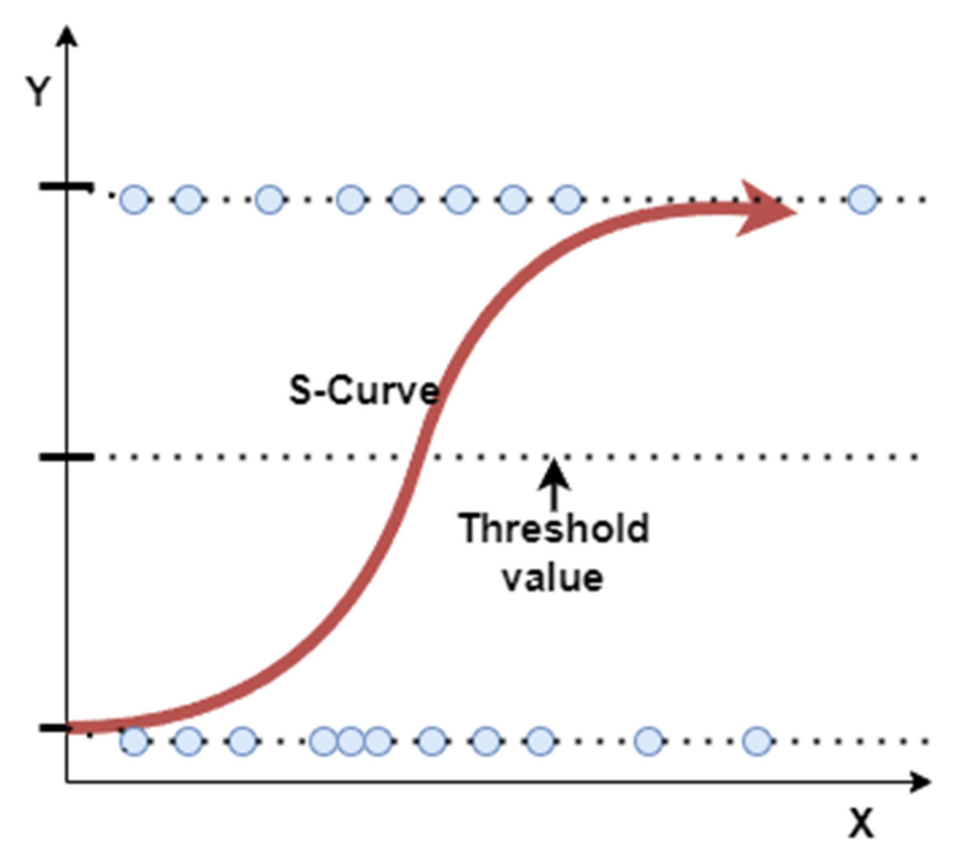
Logistic classification based on the logistic regression model assumes the classification (separation) of data using a logistic function to model the dependent variable. The dependent variable is dichotomous in nature, i.e., there could only be two possible classes therefore the method is used to classify binary data (such as malignant and benign cancer lesions). Both the target variable and the dependent variable can only take two values (logical 0 or 1). Using a logistic function, the relationship between multiple predictors and a binary target variable is modeled.

The determined function can be represented graphically as a line or an n-dimensional plane separating points from two different classes as shown in Figure 3.

4.3.2. K-Nearest Neighbor

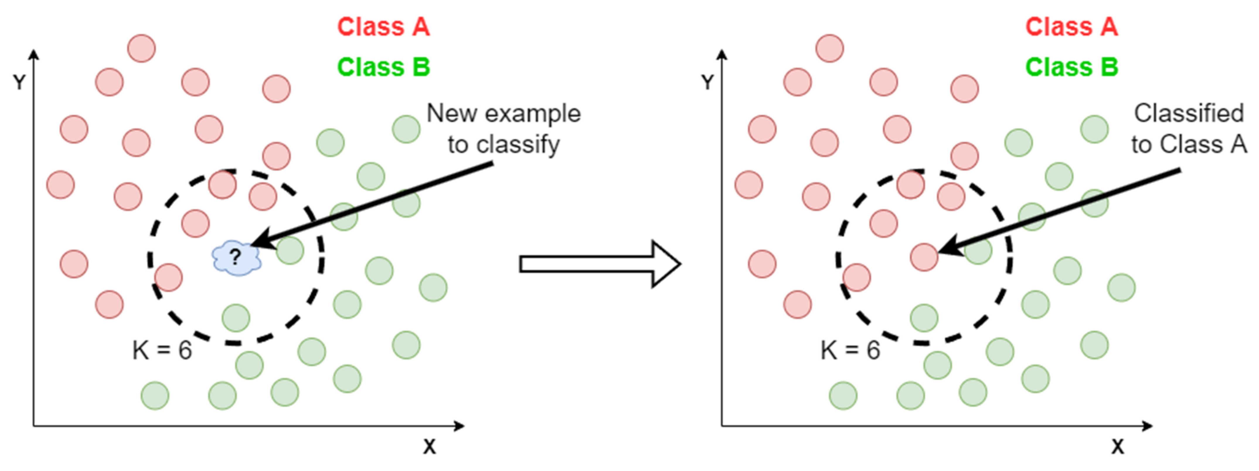
The k-Nearest Neighbors algorithm can be used to solve both classification and prediction problems. It is often called a lazy learning algorithm because it does not have a specialized learning phase and uses all training data during classification. It is a nonparametric regression algorithm. The main assumption of the algorithm is the idea of data similarity determined by the distance between points in space—data that are similar to each other (belonging to the same class) are close to each other in space. The principle of operation of the algorithm assumes that for each point in space, the distance between the query point and the remaining points is calculated, then the distances are sorted in ascending order. The first K distances and their associated labels are selected from the ordered set. The mode value of the K labels is returned as a result. The scheme of the algorithm operation is shown in Figure 4.

4.3.3. Naïve Bayes

The Naive Bayes classifier is a simple probabilistic classifier based on the assumption of mutual independence of variables. The probability model is a conditional model derived from Bayes’ theorem:

$$P\left(A|B\right)=\frac{P\left(B|A\right)P\left(A\right)}{P\left(B\right)}$$

(2)

where:

• $P\left(A|B\right)$—conditional probability; the likelihood of event A occurring given that event B occurred,
• $P\left(B|A\right)$—conditional probability; the likelihood of event B occurring given that event A occurred,
• $P\left(A\right)$, $P\left(B\right)$—probabilities of observing A and B.

When solving the classification problem, two assumptions are made. Firstly, all features affecting the classification of a given class are independent and secondly, all features have an equal impact on the result. In the formula above, variable A is a class variable that determines whether a given photo shows a benign or malignant skin lesion, based on the data of the features represented by variable B.

4.3.4. Decision Tree

Decision trees in machine learning are most often used to extract information from a set of examples, i.e., objects described with attributes that are assigned a specific decision. They are mainly used in classification problems, but they can also be adapted to solve regression problems. Unlike the Bayes classifier, which belongs to a probabilistic model, a decision tree presents a rule-based approach. Starting from the root node, which represents the entire analyzed data set, the decision tree divides it into two or more child nodes (decision nodes, sub-nodes). Creating sub-nodes increases the homogeneity, which means that the purity of the node increases relative to the target variable. The decision tree split the nodes into all available variables and then selects the splits that results in the most homogeneous sub-nodes. The selection of the algorithm used to make decisions depends on the type of target variables and it influences the final accuracy of the algorithm. A solution that is frequently explored is the CART (Classification And Regression Tree) algorithm.

4.3.5. Random Forest

The random forest algorithm is based on the use of multiple decision trees, which translates into greater accuracy of the model than in the case of using single decision trees. Each individual tree in a random forest returns a prediction of belonging to the selected class, and the class with the most votes becomes the final prediction of the model.

4.3.6. Support Vector Machine

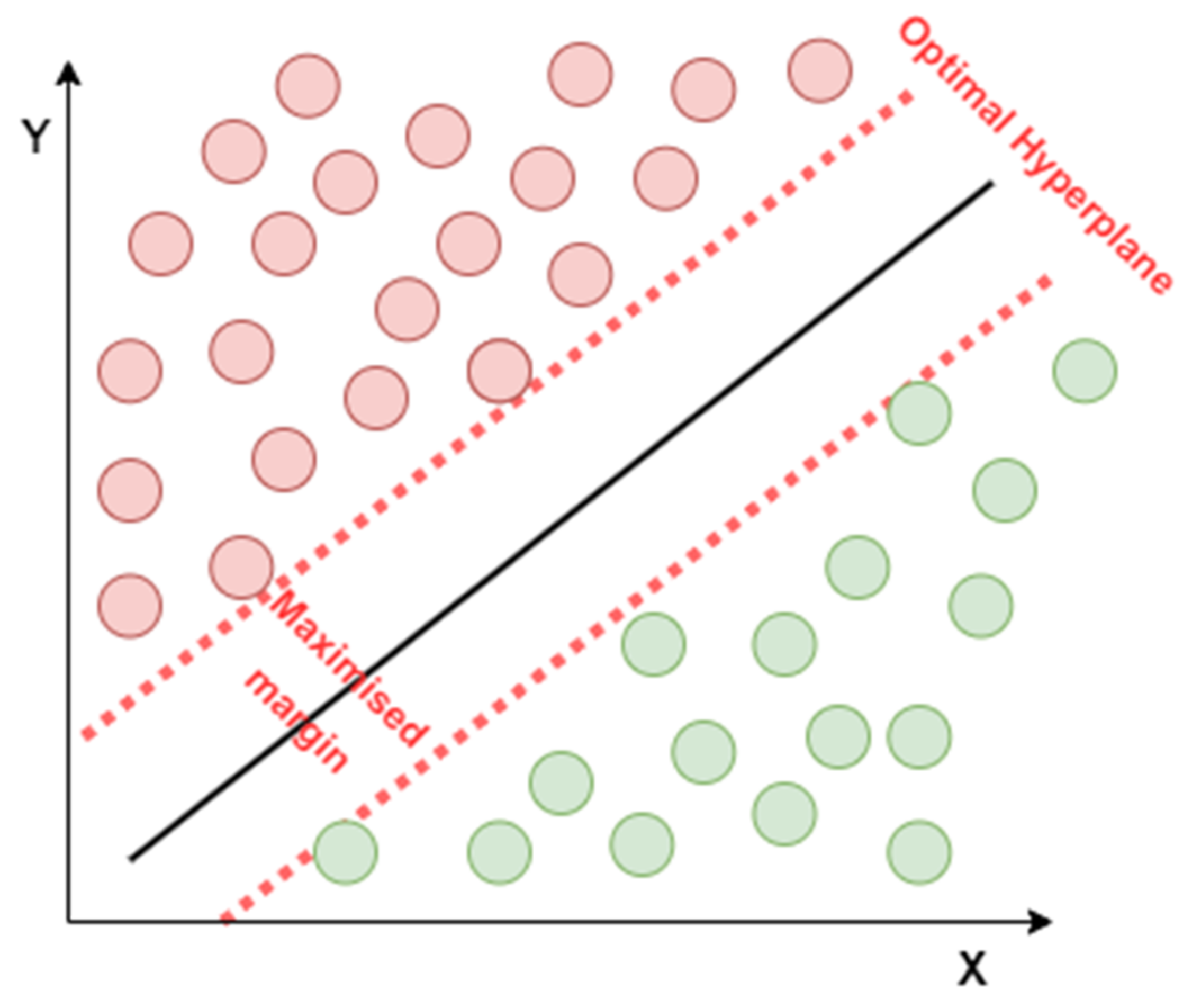
Support Vector Machine (SVM) classifier is tasked with finding the hyperplane in n-dimensional space that best classifies data belonging to two classes. The algorithm searches for hyperplanes with the maximum separating margin, i.e., the maximum distance between the closest points of each class. The hyperplane defines the decision boundaries that allow the classification of the data. Points that are on either side of the hyperplane are assigned to different classes. The scheme of the algorithm operation is shown in Figure 5.

In the next step, obtained results have been compared with results received using deep learning models. For this purpose, several pre-trained models were tested—VGG-16 [29], Inception-v3 [30], Inception-ResNet-v2 [31] and ResNet-50 [25]. Each model previously trained on the ImageNet dataset [32] has been tuned using training data and then tested on the test dataset.

The data has been pre-processed before the training, i.e., converted to one fixed size of 200 × 200 pixels and for the training data, several transformations were used to avoid the overfitting phenomenon due to the relatively small data pool.

5. Results

This section presents the results of the conducted experiments. To quantify the effectiveness of models, 4 basic machine learning metrics were determined: accuracy (acc), precision (prec), recall, and F1-score (F1).

$$acc=\frac{correctly classified casses}{all cases}$$

(3)

$$prec=\frac{correctly classified malignant cases}{all cases classified as malignant}$$

(4)

$$recall=\frac{correctly classified malignant cases}{all malignant cases}$$

(5)

$$F1=2·\frac{prec·recall}{prec+recall }$$

(6)

When solving problems in the field of medical diagnosis, the FN (False Negative) index is very important which affects the value of the denominator of the recall. The analyzed issue, it corresponds to a situation where a malignant skin lesion was incorrectly diagnosed as benign. It is therefore important that the value of the FN index is as low as possible because it is the worst type of error. Due to this, in the further evaluation of the quality of machine learning algorithms, mainly accuracy and recall were taken into account.

To evaluate the performance of individual algorithms, the training time of a given algorithm was assessed, and in the case of classic machine learning algorithms, also the time necessary to perform feature extraction with the use of a given descriptor. All computations were performed using Python 3.7.10 and machine learning tools: TensorFlow 2.4.1 and Scikit-Learn 0.22.2. All neural networks were trained for 20 epochs (estimated value needed to obtain the convergence for all models) using the Adam optimizer with a learning rate equal to lr = 0.0005.

5.1. Classic Machine Learning Algorithms

Figure 6 shows the highest values of accuracy and recall metrics achieved by each of the analyzed algorithms.

The Random Forest algorithm turned out to be the most effective algorithm for the automatic detection of cancer lesions. Accuracy of 86.36% was obtained using training data extracted from the Histogram, Haralick, and Hu Moments descriptors combination, and the recall of 95% using the Histogram, LBP, and Haralick descriptors combination. Naive Bayes achieved the highest recall—100%, but with much lower accuracy.

Table 1. Comparison of the obtained results for various machine learning algorithms.

Algorithm	Accuracy, %	Descriptor for Accuracy	Recall, %	Descriptor for Recall
Logistic Regression	82.12	Histogram_LBP_Haralick_ _HuMoments	85.00	Histogram_LBP_HuMoments
		Histogram_LBP_Haralick		Histogram_LBP
		Histogram_Haralick_ _HuMoments		Histogram
				Histogram_ HuMoments
	81.82	Histogram_Haralick	84.00	Histogram_LBP_Haralick_ _HuMoments
	79.85	Histogram		Histogram_LBP_Haralick
				Histogram_Haralick_ _HuMoments
k-Nearest Neighbors	80.00	Histogram_LBP_Haralick_ _HuMoments	78.67	Histogram_LBP_HuMoments
				Histogram_LBP
				Histogram_LBP_Haralick
	79.70	Histogram_LBP_Haralick	78.00	Histogram_Haralick
		Histogram_LBP		Histogram_Haralick_ _HuMoments
Naive Bayes	74.09	Histogram_Haralick	100	HuMoments
		Histogram_LBP_Haralick		Haralick_HuMoments
		Histogram_LBP		LBP_Haralick_HuMoments
		Histogram
	69.85	LBP_Haralick	99.67	Histogram_Haralick_ _HuMoments
				Histogram_LBP_Haralick_ _HuMoments
		LBP_HuMoments		Histogram_ HuMoments
				Histogram_LBP_HuMoments
Decision Tree	78.18	Histogram_Haralick	75.33	Histogram_Haralick
	78.03	Histogram_LBP	74.33	Histogram_LBP_Haralick
		Histogram		Histogram
				Haralick_HuMoments
Random Forest	86.36	Histogram_Haralick_ _HuMoments	95.00	Histogram_LBP_Haralick
	85.45	Histogram_LBP_HuMoments	94.67	Histogram_Haralick_ _HuMoments
SVM	82.42	Histogram_Haralick	93.00	Histogram_ HuMoments
	81.97	Histogram_LBP_Haralick_ _HuMoments	91.00	Histogram_LBP_HuMoments

summarizes the highest acc and recall values for each classification algorithm, including the descriptor or combination of descriptors used.

For each algorithm, the most effective set of diagnostic features was defined, which allowed forobtaining the highest value of accuracy and recall for the test set. The best results were achieved using a combination of descriptors containing a color descriptor (Histogram). The most effective combination of diagnostic features turned out to be the Histogram-LBP-Haralick combination, which appeared in the top 5 highest scores both in terms of accuracy and recall the most often (9 times).

Similarly, the self-used Hu Moments and LBP descriptors (11 and 10 occurrences among the lowest results, respectively) were considered to be the worst descriptors of diagnostic features for this problem. When used alone, they achieved very low results, however, in combination with other feature descriptors, they increased the accuracy and recall values for the analyzed case by a dozen or so percentage points.

5.2. Comparison with Deep Learning Algorithms

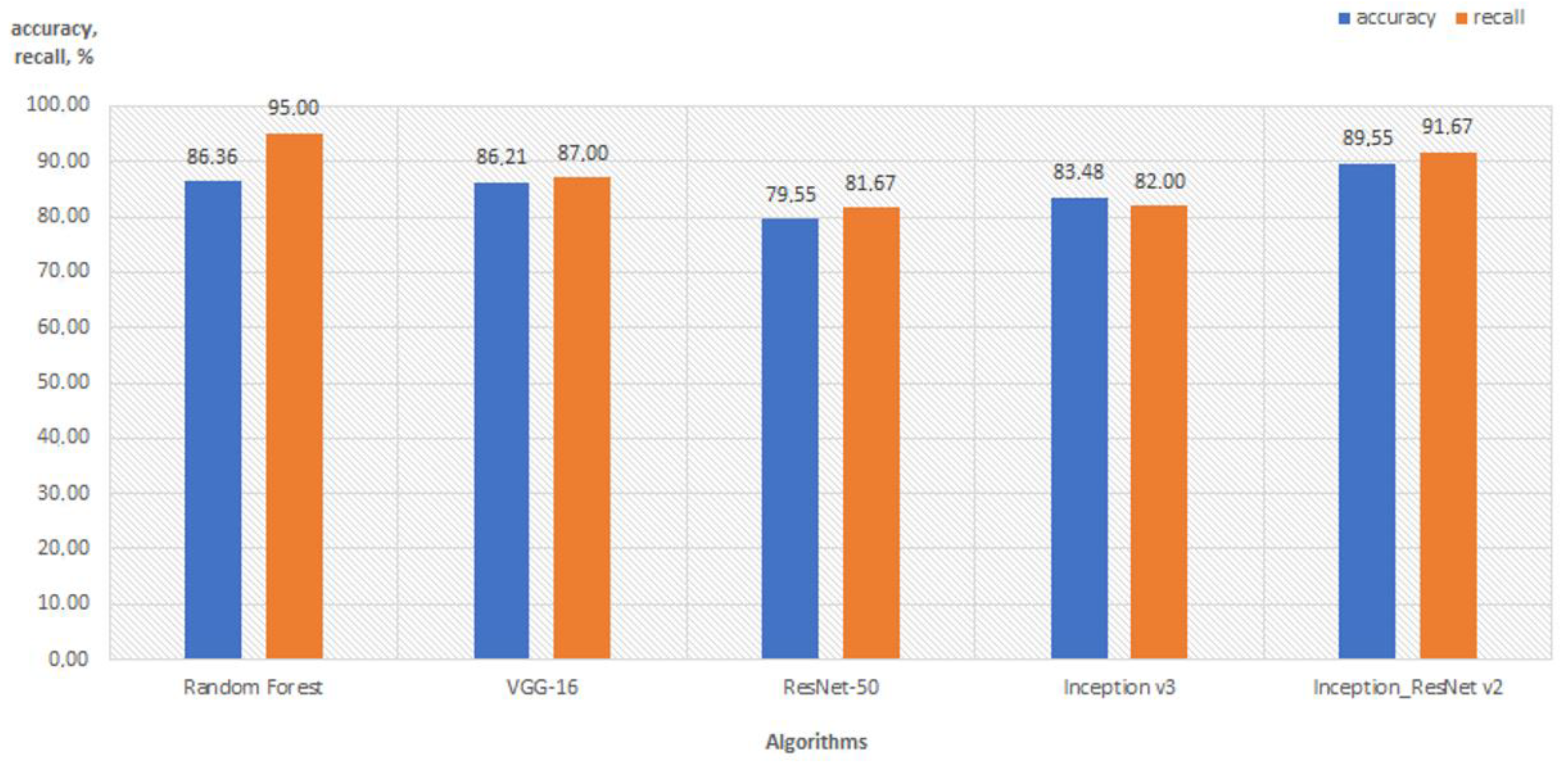
Figure 7 shows a comparison of results obtained for the best option of the traditional classifier—the Random Forest classifier with features obtained from combination Histogram-LBP-Haralick, and neural networks models.

Results show that traditional machine learning algorithms using suitable feature descriptors can obtain better results in digital image classification than various types of CNNs. Model Inception ResNet v2 achieved results closest to Random Forest classifier, but slightly worse—accuracy equals 89.55% and recall equals 91.67%. The decisive factor influencing the obtained results was the size of the training data set. Machine learning models are more efficient in the training process with a small dataset. In neural networks, there is a problem of overfitting which was most noticeable in the case of the most complex model—ResNet-50. Overfitting shows very low loss and high accuracy for the training set and much worse values for the validation or test sets. During the experiment, modifications were used to reduce overfitting—data augmentation for all models and regularization using the L1 and L2 norms for the ResNet architecture which are not necessary for machine learning algorithms.

5.3. Comparative Analysis of Performance and Effectiveness

Table 2. Comparison of learning time of algorithms.

Algorithm	Time, s
Logistic Regression_ Histogram_LBP_Haralic_HuMoments	53.50
k-Nearest Neighbors_ Histogram_LBP_Haralic_HuMoments	31.09
Naive Bayes_Histogram_Haralick	22.35
Decision Tree_ Histogram_Haralick	22.78
Random Forest_ Histogram_Haralick_ _HuMoments	22.97
SVM_ Histogram_Haralick	26.72
VGG-16	749.00
ResNet-50	615.00
InceptionV3	612.00
ResNet-InceptionV2	800.00
Histogram	0.5
Haralick	21.8
Hu Moments	0.16
LBP	8.7

summarizes the learning time values of the individual algorithms presented in Section 5.1 and Section 5.2 until convergence. For the algorithms in Section 5.1, only the training time for the most efficient algorithm in terms of accuracy is shown. The time necessary to perform feature extraction with the use of the selected descriptor or their combinations has also been added to the training time. The feature extraction time for each descriptor is shown at the end of the table.

The learning time in the case of deep learning algorithms is several to several dozen times longer than in the case of classic machine learning algorithms. This is due to the necessity to perform successive repetitions of the learning epochs necessary for the algorithm to converge. However, longer training time does not translate into an increase in the efficiency of the algorithm, on the contrary—the Random Forest model with a much shorter training time achieves higher values of classification metrics than the analyzed neural networks.

6. Conclusions

The paper presents a comparison of machine learning algorithms applied to the automatic diagnosis of skin lesions classified as benign or malignant (cancerous). The input data for the classifiers were vectors of diagnostic features obtained through the use of shape, color, and texture descriptors. As part of the research, for each algorithm, the most optimal set of diagnostic features was defined, allowing for the achievement of the highest values of accuracy and recall metrics for the set of test data. The Random Forest classifier obtained the best result. The algorithm also turned out to be more efficient than Convolutional Neural Networks, fine-tuned using an analyzed dataset. Further work on the presented research results is planned, including:

• extending the pre-processing of images with the segmentation operation to reduce the background influence on the obtained results;
• extending the database of used feature descriptors, and comparison of their impact on the effectiveness and performance of algorithms.

References

1. Davis, L.E.; Shalin, S.C.; Tackett, A.J. Current state of melanoma diagnosis and treatment. Cancer Biol. Ther. 2019, 20, 1366–1379. [Google Scholar] [CrossRef] [PubMed] [Green Version]
2. MacGill, M. What to Know about Melanoma. Medical News Today. Available online: https://www.medicalnewstoday.com/articles/154322 (accessed on 15 September 2022).
3. Heistein, J.B.; Archarya, U. Malignant Melanoma. StatPearls. Available online: https://www.statpearls.com/ArticleLibrary/viewarticle/24678 (accessed on 15 September 2022).
4. Blundo, A.; Cignoni, A.; Banfi, T.; Ciuti, G. Comparative Analysis of Diagnostic Techniques for Melanoma Detection: A Systematic Review of Diagnostic Test Accuracy Studies and Meta-Analysis. Front. Med. 2021, 8, 637069. [Google Scholar] [CrossRef] [PubMed]
5. Silva, T.A.E.d.; Silva, L.F.d.; Muchaluat-Saade, D.C.; Conci, A.A. Computational Method to Assist the Diagnosis of Breast Disease Using Dynamic Thermography. Sensors 2020, 20, 3866. [Google Scholar] [CrossRef] [PubMed]
6. Fanizzi, A.; Losurdo, L.; Basile, T.M.A.; Bellotti, R.; Bottigli, U.; Delogu, P.; Diacono, D.; Didonna, V.; Fausto, A.; Lombardi, A.; et al. Fully Automated Support System for Diagnosis of Breast Cancer in Contrast-Enhanced Spectral Mammography Images. J. Clin. Med. 2019, 8, 891. [Google Scholar] [CrossRef] [PubMed] [Green Version]
7. Sieczkowski, K.; Sondej, T.; Dobrowolski, A.; Olszewski, R. Autocorrelation algorithm for determining a pulse wave delay. In Proceedings of the 2016 Signal Processing: Algorithms, Architectures, Arrangements, and Applications (SPA), Poznan, Poland, 21–23 September 2016; pp. 321–326. [Google Scholar] [CrossRef]
8. Hasan, M.J.; Shon, D.; Im, K.; Choi, H.-K.; Yoo, D.-S.; Kim, J.-M. Sleep State Classification Using Power Spectral Density and Residual Neural Network with Multichannel EEG Signals. Appl. Sci. 2020, 10, 7639. [Google Scholar] [CrossRef]
9. Hasan, M.J.; Kim, J.-M. A Hybrid Feature Pool-Based Emotional Stress State Detection Algorithm Using EEG Signals. Brain Sci. 2019, 9, 376. [Google Scholar] [CrossRef] [PubMed] [Green Version]
10. Lin, Y.; Xie, H. Face Gender Recognition based on Face Recognition Feature Vectors. In Proceedings of the 2020 IEEE 3rd International Conference on Information Systems and Computer Aided Education (ICISCAE), Dalian, China, 27–29 September 2020; pp. 162–166. [Google Scholar] [CrossRef]
11. Alay, N.; Al-Baity, H.H. Deep Learning Approach for Multimodal Biometric Recognition System Based on Fusion of Iris, Face, and Finger Vein Traits. Sensors 2020, 20, 5523. [Google Scholar] [CrossRef] [PubMed]
12. Kanimozhi, S.; Gayathri, G.; Mala, T. Multiple Real-time object identification using Single shot Multi-Box detection. In Proceedings of the 2019 International Conference on Computational Intelligence in Data Science (ICCIDS), Gurugram, India, 6–7 September 2019; pp. 1–5. [Google Scholar] [CrossRef]
13. Rapacz, S.; Chołda, P.; Natkaniec, M. A Method for Fast Selection of Machine-Learning Classifiers for Spam Filtering. Electronics 2021, 10, 2083. [Google Scholar] [CrossRef]
14. Xia, H.; Wang, C.; Yan, L.; Dong, X.; Wang, Y. Machine Learning Based Medicine Distribution System. In Proceedings of the 2019 10th IEEE International Conference on Intelligent Data Acquisition and Advanced Computing Systems: Technology and Applications (IDAACS), Metz, France, 18–21 September 2019; pp. 912–915. [Google Scholar] [CrossRef]
15. Ullrich, M.; Küderle, A.; Reggi, L.; Cereatti, A.; Eskofier, B.M.; Kluge, F. Machine learning-based distinction of left and right foot contacts in lower back inertial sensor gait data. In Proceedings of the 2021 43rd Annual International Conference of the IEEE Engineering in Medicine & Biology Society (EMBC), Mexico City, Mexico, 1–5 November 2021; pp. 5958–5961. [Google Scholar] [CrossRef]
16. Seif, G. Deep Learning vs. Classical Machine Learning. Available online: https://towardsdatascience.com/deep-learning-vs-classical-machine-learning-9a42c6d48aa (accessed on 9 April 2021).
17. Jianu, S.R.S.; Ichim, L.; Popescu, D. Automatic Diagnosis of Skin Cancer Using Neural Networks. In Proceedings of the 2019 11th International Symposium on Advanced Topics in Electrical Engineering (ATEE), Bucharest, Romania, 28–30 March 2019; pp. 1–4. [Google Scholar] [CrossRef]
18. Weiss, K.; Khoshgoftaar, T.M.; Wang, D. A survey of transfer learning. J. Big Data 2016, 3, 1–40. [Google Scholar] [CrossRef] [Green Version]
19. Pillay, V.; Hirasen, D.; Viriri, S.; Gwetu, M. Melanoma Skin Cancer Classification Using Transfer Learning. In Advances in Computational Collective Intelligence. ICCCI 2020. Communications in Computer and Information Science; Hernes, M., Wojtkiewicz, K., Szczerbicki, E., Eds.; Springer: Cham, Switzerland, 2020. [Google Scholar] [CrossRef]
20. Vasconcelos, C.N.; Vasconcelos, B.N. Convolutional neural network committees for melanoma classification with classical and expert knowledge based image transforms data augmentation. arXiv 2017, arXiv:1702.07025. [Google Scholar]
21. Huang, H.W.; Hsu, B.W.Y.; Lee, C.H.; Tseng, V.S. Development of a light-weight deep learning model for cloud applications and remote diagnosis of skin cancers. J. Dermatol. 2020, 48, 310–316. [Google Scholar] [CrossRef] [PubMed]
22. Sabri, M.A.; Filali, Y.; el Khoukhi, H.; Aarab, A. Skin Cancer Diagnosis Using an Improved Ensemble Machine Learning model. In Proceedings of the 2020 International Conference on Intelligent Systems and Computer Vision (ISCV), Fez, Morocco, 9–11 June 2020; pp. 1–5. [Google Scholar] [CrossRef]
23. Tumuluru, P.; Lakshmi, C.P.; Sahaja, T.; Prazna, R. A Review of Machine Learning Techniques for Breast Cancer Diagnosis in Medical Applications. In Proceedings of the 2019 Third International conference on I-SMAC (IoT in Social, Mobile, Analytics and Cloud) (I-SMAC), Palladam, India, 12–14 December 2019; pp. 618–623. [Google Scholar] [CrossRef]
24. Yu, Z.; Jiang, X.; Zhou, F.; Qing, J.; Ni, D.; Chen, S.; Lei, B.; Wang, T. Melanoma Recognition in Dermoscopy Images via Aggregated Deep Convolutional Features. IEEE Trans. Biomed. Eng. 2019, 66, 1006–1016. [Google Scholar] [CrossRef] [PubMed]
25. He, K.; Zhang, X.; Ren, S.; Sun, J. Deep residual learning for image recognition. In Proceedings of the IEEE Conference on Computer Vision and Pattern Recognition (CVPR), Las Vegas, NV, USA, 27–30 June 2016; pp. 770–778. [Google Scholar]
26. The International Skin Imaging Collaboration. Available online: https://www.isic-archive.com/#!/topWithHeader/wideContentTop/main (accessed on 5 January 2021).
27. Vadivel, A.; Sural, S.; Majumdar, A.K. Human color perception in the HSV space and its application in histogram generation for image retrieval. In Proceedings of the Color Imaging X: Processing, Hardcopy, and Applications, San Jose, CA, USA, 17 January 2005; Volume 5667. [Google Scholar] [CrossRef]
28. Ojala, T.; Pietikainen, M.; Harwood, D. Performance evaluation of texture measures with classification based on Kullback discrimination of distributions. In Proceedings of the 12th International Conference on Pattern Recognition, Jerusalem, Israel, 9–13 October 1994; Volume 1, pp. 582–585. [Google Scholar] [CrossRef]
29. Simonyan, K.; Zisserman, A. Very Deep Convolutional Networks for Large-Scale Image Recognition. arXiv 2014, arXiv:1409.1556. [Google Scholar]
30. Szegedy, C.; Vanhoucke, V.; Ioffe, S.; Shlens, J.; Wojna, Z. Rethinking the Inception Architecture for Computer Vision. In Proceedings of the 2016 IEEE Conference on Computer Vision and Pattern Recognition (CVPR), Las Vegas, NV, USA, 27–30 June 2016; pp. 2818–2826. [Google Scholar]
31. Szegedy, C.; Ioffe, S.; Vanhoucke, V.; Alemi, A.A. Inception-v4, inception-ResNet and the impact of residual connections on learning. In Proceedings of the Thirty-First AAAI Conference on Artificial Intelligence (AAAI’17), San Francisco, CA, USA, 4–9 February 2017; pp. 4278–4284. [Google Scholar]
32. Deng, J.; Dong, W.; Socher, R.; Li, L.-J.; Li, K.; Li, F.-F. Imagenet: A large-scale hierarchical image database. In Proceedings of the 2009 IEEE Conference on Computer Vision and Pattern Recognition, Miami, FL, USA, 20–25 June 2009; pp. 248–255. [Google Scholar]
Figure 1. Sample imaging of skin cancer: (a)—benign lesion, (b)—malignant lesion [26].
Applsci 12 09960 g001
Figure 2. Flowchart of proposed method.
Applsci 12 09960 g002
Figure 3. The idea of logistic regression separating variables into two classes.
Applsci 12 09960 g003
Figure 4. The idea of K-Nearest Neighbor algorithm.
Applsci 12 09960 g004
Figure 5. The idea of Support Vector Machine.
Applsci 12 09960 g005
Figure 6. Accuracy and recall of machine learning algorithms.
Applsci 12 09960 g006
Figure 7. Comparison of Random Forest Classifier and deep earning algorithms.
Applsci 12 09960 g007