Benchmarking of Load Forecasting Methods Using Residential Smart Meter Data

Abstract

As the access to consumption data available in household smart meters is now very common in several developed countries, this kind of information is assuming a providential role for different players in the energy sector. The proposed study was applied to data available from the Smart Meter Energy Consumption Data in the London Households dataset, provided by UK Power Networks, containing half-hourly readings from an original sample of 5567 households (71 households were hereby carefully selected after a justified filtering process). The main aim is to forecast the day—ahead load profile, based only on previous load values and some auxiliary variables. During this research different forecasting models are applied, tested and compared to allow comprehensive analyses integrating forecasting accuracy, processing times and the interpretation of the most influential features in each case. The selected models are based on Multivariate Adaptive Regression Splines, Random Forests and Artificial Neural Networks, and the accuracies resulted from each model are compared and confronted with a baseline (Naïve model). The different forecasting approaches being evaluated have been revealed to be effective, ensuring a mean reduction of 15% in Mean Absolute Error when compared to the baseline. Artificial Neural Networks proved to be the most accurate model for a major part of the residential consumers.

1. Introduction

Smart meter data have already proved their importance for different players in the electricity sector. On the one hand, the transmission and distribution operators may have access to individual load profiles, allowing the estimation of future load demand for different areas. They provide the physical balance between supply and demand (at real time), and the opportunity to adjust the grid operation to minimize power losses, voltage drops (or other power quality events), thus increasing the grid resilience and reducing costs. For suppliers, it is also valuable to know in detail how the clients are effectively using this resource, estimating the expected accumulated electricity volume for their customer portfolio (at different hourly periods) when buying in the electricity market. Suppliers may also propose different commercial options (such as contracted power, the choice between flat/time of use/ or dynamic rates or even the counting cycles programmed in the meters) according to each consumer profile, launching fair rates, obtaining a distinct and valuable position as electricity retailers. Even end-users also take advantage of getting access to their own consumption, which should be viewed as a trigger to make demand more flexible, as this detailed information may undoubtedly increase awareness (when there are untypical consumptions, since alarmistic solutions are becoming popular). Furthermore, with the increasing and desired investment in renewable sources, traditional consumers are becoming prosumers and this phenomenon is expected to increase the interest of residential consumers (but not restricted to this sector) to rethink consumption behaviour, trying to match consumption with the available electricity from self-generation. The consequences are less dependence on electricity provided by the grid, with the inherent savings in energy bills and the reduction in greenhouse gas (GHG) emissions.

Through a comprehensive analysis of works developed in this domain, it becomes clear that several authors have made use of machine learning applications to estimate hourly electricity consumptions for the day-ahead, not only at a considerable aggregation level, but at a single household as well. Some references still use traditional statistical methods, such as Linear [1] or Polynomial Regression, Autoregressive Integrated Moving Average—ARIMA models [2,3,4] or some variants (such as incremental ARIMA or involving a prior stage of signal pre-processing) to enhance their performance. In [5], a model based on Conditional Kernel Density Estimation is compared with machine learning models. Despite the interest associated with these simple approaches, there are some drawbacks often referred to, such as the effect of multicollinearity among the input variables being used [6], and the models tend to become hostage and sensitive to the data quality, which is quite difficult to preserve in this kind of data series [7].

Machine learning algorithms tend to be transversal to a major part of the analysed references. In this domain, Artificial Neural Networks (ANN) are, by far, the most used algorithms [8]. This popular approach is a data-driven method [9] that does not need to be explicitly programmed [10]. ANN are often pointed out by their ability to learn and to identify hidden trends, thereby finding the intrinsic trends in time series [11]. Their ability to generalize even in the presence of incomplete and noisy data (common in residential smart meter data) [10] and their non-parametric distinction (they do not require prior assumptions about the data distribution) make them good approximators capable to model any continuous function at any desired accuracy. Some drawbacks associated with the use of ANNs in forecasting applications are the risk of getting underfitted (as it can get stuck on a local optimal solution) or overfitted models (if the training process is not interrupted through a proper cross-validation strategy) [12]. Thus, the practical difficulty is to accurately find the weights associated with each connection along the training process [11]. Another disadvantage of their use is the lack of explanatory variables, making them lose interpretability and explainability (also known as the black-box problem) [10]. In [9], it is mentioned that shallow ANN architectures may assume that inputs/outputs are independent of each other, even when dealing with sequential data. To overcome that fact, recent research is adopting novel methodologies based on deep learning. Recurrent Neural Networks (RNN) are one of the alternatives more adapted to time series data, using feedback connections among the nodes to remember the values from the previous time steps [9]. Nevertheless, long sequences may cause serious problems that may be overcome by using Long Short-term memory networks (LSTM), a variant of RNN. LSTM use internal memories to store information and are faster to converge. Even with this apparent research potential, some authors [13] have concluded that LSTM have limited improvements in accuracy when applied to residential smart meter data, are quite more complicated and more time-consuming, and are not feasible for daily use in practice. Ref. [14] have tested Convolutional Neural Networks, LSTM and Bidirectional LSTM, being identified as challenging when tested alone, and the resulting training times are inconsistent due to various customer load profiles and different factors such as dataset sizes, number of features and prediction model parameters. Ref. [15] also compared deep learning approaches with more usual models (Linear Regression, Random Forest (RF), K-Nearest Neighbours and Support Vector Regression (SVR)). Ref. [16] also compared LSTM models with ANN, SVR and RF applied to a dataset involving Irish homes and businesses and assumed that error bars have less variance in MAPE metrics in more “old-fashioned” models (ANN, SVR and RF), while in LSTM approaches MAPE vary by up to 11% in the five models run. Ref. [17] also concluded that Convolutional Neural Networks present some difficulties to predict spikes, as they exploit the temporal stationarity of load time series.

In the subset of machine learning, other popular methods have been applied in the last few years, such as Support Vector Machines, Decision Trees and Random Forests [1,12,18,19]. These approaches are also quite common to be proposed or to be used as benchmarks in comparative analysis. Support Vector Machines are based on a structural risk minimization principle, rather than an empirical risk minimization principle that characterizes ANN models [5,9,11]. Their use is based on kernels, leading to the absence of local minima. They allow a considerable control of the process (acting on the tolerance margin or on the support vectors), being less dependent on the dimensionality of the feature space. The major challenge is the inherent combinatorial effort to fine tune the hyperparameters (error margin, penalty factor and kernel constant). Some authors propose metaheuristics to guide this search, while others explore simpler approaches such as a grid search technique [5]. Decision Trees are interesting for use when time series with missing values are presented, as they can handle numerical data and categorical information [19], which makes them very attractive models for various applications. Random Forest is an extension of Decision Trees, as it uses multiple models to improve its performance, rather than using a single tree model [19]. Random Forest runs efficiently on large amounts of data, tends to provide high accuracy [18] and has low sensitivity to parameter values, as it has an inherent internal cross-validation [12]. The most interesting advantage is a suitable variable importance measure. The drawback often pointed out is the hard task to find an optimal architecture and parameter tuning [9,12,18] (predefining the total number of trees, the maximum number of variables for decision splits or the minimum number of records for leaf nodes).

The use of ensemble methods is being substantially considered in the bibliography. Ref. [20] propose the combination of ANN with RF models, ref. [21] combines RF with Linear Regression and ref. [18] propose a hybrid method combining Random Forest and Multilayer Perceptron. An ensemble method combining several single models including Auto-regressive, Multilayer Perceptron, Extreme Learning Machine, Radial Basis Function and Echo-State Network is proposed by [7]. Refs. [14,15] combine different approaches involving deep learning. Despite the generic trend to improve forecasting accuracy, hybrid methods are considerably more time-consuming (when scalability has a key role) and lacks for interpretability and explainability.

Regarding error metrics, it is quite controversial to compare different works, as the datasets are obtained in different parts of the world (as access to smart meter data is becoming a reality in several developed countries) and the consumption patterns and volumes can be quite distinct. Ref. [11] describes Mean Squared Errors from 0.1 to 0.13 kWh² for different hours being predicted and an accuracy from 52% to 70% (assuming a tolerance error within 10%). Ref. [21] reveal a Root Mean Squared Error of about 0.704 kW when predicting active power for the day-ahead with 15 min resolution. Ref. [14] shows Mean Absolute Percentage errors varying from 55.8% to 36.75% with the proposed hybrid model. Ref. [7] noted a reduction from 15.7% to 13.54% in the Mean Absolute Percentage Error metric when applying their proposed ensemble method. Ref. [22] proposes a federated learning algorithm with recurrent neural networks conducted with residential consumers, leading to a MAPE of about 17%.

Different research has been applied in this domain, highlighting the importance of finding suitable forecasting models to be applied at household consumption level. Due to the inherent randomness and noise associated with residential consumption profiles, this task is often considered more challenging than forecasting at a level with more consumption aggregation (such as that of a public substation or even a national transmission grid).

The main contributions of this study can be summarized as follows:

-

A comparison among different forecasting approaches: different alternatives were chosen to allow accurate predictions, also being interpretable models, providing feasible training times and easy to replicate.

-

A comparison between different alternatives not applied to a single consumer with specific characteristics, but for a larger number of consumers to allow a fair and extended comparison of created models: load patterns available in the used dataset are diverse; thus, scalability and flexibility are providential tools for the proposed forecasting methods.

-

A detailed analysis of the created forecasting models, allowing the interpretation of the different feature contributions and a comparison of the training times.

The article is organized as follows: Section 2 describes the used dataset for this study and presents some background related to the used methods and the strategies adopted when applying them in this study, and the list of features considered is also introduced. Section 3 is initiated with the description of the adopted error metrics, followed by the main results presentation, providing a detailed comparison among the proposed methods and allowing a comprehensive analysis of the main influential features in each case. Finally, in Section 4, the main conclusions are drawn, revealing the potential amongst the forecasting models tested and highlighting a comparative analysis of these selected models. In this section, some topics are proposed for further research.

2. Materials and Methods

In this section, the used dataset is carefully described to allow the comprehension of the assumptions associated with this choice. Furthermore, the different forecasting approaches are theoretically presented, as well as the description of the training/validation/test subset split and the inputs’ selection phase.

2.1. Used Dataset

The dataset used is related with energy consumption readings for a sample of 5567 London households between November 2011 and February 2014. These readings carried out from UK Power Networks within the scope of the Low Carbon London project (here called the LCL dataset) [23]. Readings were taken at half hourly intervals and represent the total electricity consumption for that period in kWh. Despite a large number of consumers available in this study, the authors carefully analysed the dataset and imposed specific assumptions to ensure representative and reliable data. The following rules were created to select the consumers who contribute with data to be used in the further phase related to forecasting application.

-

The ratio of null or atypical values in the total amount of records available for the considered period (28 months) must be kept below 5%. Despite some reasons that may cause null values (such as power outages, or temporary absence of the households in the consumption locations) or may cause atypical values (outliers due to sudden and abrupt changes typically caused by data transmission/communication problems), it is important to preserve data integrity to enhance the forecasting exercise.

-

For each consumer, the consumption trend should be kept uniform for the different complete civil years available. It is expected that consumption variations may occur during the year due to seasonality effect, but significant changes in annual total consumption may be caused by unexpected consumer behaviour changes, measurement failure or even trouble in data transmission/storage. Based on mean daily consumption, differences above 10% from year to year have triggered less uniformity in the consumption trend.

After this filtering process, the dataset was considerably summarized to 71 consumers, providing large confidence in the quality of available data (for almost the whole period between November 2011 and February 2014, as some initial and final periods of data were not clearly trustworthy). In the authors’ opinion, this selected sample is representative enough to be explored, allowing a benchmark among the proposed forecasting tools.

Table 1. Summary of the available dataset and the selected sample.

Data Description	Number of Consumers	Available Data
Original Data	5567	From 1 November 2011 to 28 February 2014
Selected Sample	71	From 21 December 2011 to 27 February 2014 1

¹ The last day of February 2014 presented several null values for the 71 selected consumers; thus, it was not considered.

summarises the LCL dataset available information, and the selected sample used.

2.2. Forecasting Approaches

As mentioned before, due to a considerable amount of noise in the consumption time series for each individual consumer, and in order to create methodologies to deal with a large number of individual end-users, it is strongly recommended to create forecasting models simultaneously accurate, straightforward, non-time-consuming and even explainable. This research uses Multivariate Adaptive Regression Splines, Random Forest and Artificial Neural Networks.

2.2.1. Multivariate Adaptive Regression Splines (MARS)

This approach is characterized as a regression algorithm and its foundations rely on simple linear regressors, making it easy to use and to interpret [13,20]. As the load demand often represents a non-linear dependence between output(s) and inputs, the MARS model can cope with it, as it involves an ensemble of aggregated linear functions based on one or two hinge functions. The perspective of hinge functions can be approximated to:

h(x − k) = max(0; x − k) = {x − k, if x > k; and 0 if x ≤ k}

(1)

where k is a constant, known as a knot. The MARS model will result in aggregating the hinge functions associated with each knot, and even considering linear dependence on single features and a bias (also known as the intercept term).

Each knot can generate one or a pair of “knees” at the model function. Figure 1 illustrates this by considering a non-linear real function in light blue and an approximation made possible by using a MARS model (in dark blue). As the two hinge functions show, two knots are here considered (x = −10 and x = 10) and each individual hinge function are enough to model this desired non-linearity.

To fine-tune the model, the associated knots must be found based on the inputs-outputs pairs provided during the training phase, being a data-driven model. Many candidate basis functions are generated in the forward phase, being generated in pairs h(x − k) and h(k − x). Each pair is added to the model if it contributes to reducing the model’s performance. A subsequent backward phase is used to prune the terms in the final equation whenever they do not contribute to the overall performance. This backward process can be viewed to avoid model overfitting, as a generalized cross-validation is applied to compare the performance of model subsets. It ensures a trade-off between accuracy and model complexity.

MARS models in the scope of this research were created and tested using PyEarth package [24] to be used in the Scikit library of Python (being a third-party library). By default, the maximum number of terms was considered as a value dependent on number of features and number of samples, with a maximum number of 1 for the terms generated by the forward pass, a value of 3.0 as penalty factor during the pruning pass and a zero tolerance.

2.2.2. Random Forest Regressor

Random Forest is characterized as an ensemble machine learning algorithm, as each tested decision tree is fit on a slightly different training dataset and uses different features, and in turn, results in a slightly different performance. An example of an individual decision tree applied in a load forecasting application is available in Figure 2.

The first step of the CART (Classification and Regression Tree) algorithm consists in splitting at best the root into two different child nodes if it implies a cost function (in general, the variance of child nodes) reduction [12]. Then, the child nodes are also divided according to the same procedure. The expansion of the tree is stopped by a termination criterion. It is common to stop the tree when a maximum number of levels has been reached, or when a node contains less than a defined number of observations [12,18].

The main principle is called bagging, where a sample of size n from the training set is selected randomly and fitted to a regression tree. This sample is called a bootstrap, and is chosen with replacement, i.e., the same observations may appear many times. A bootstrap sample is obtained by selecting randomly n observations with replacement; each observation has the probability of 1/n to be selected. The independent identically distributed random variables represent this random selection. The bagging algorithm selects several bootstrap samples, applies the CART algorithm to them to obtain a collection of predicting trees, and then aggregates the output of all these predictors.

In addition to bagging, to split a node, only a predefined number of the features are selected, and the RF algorithm tries to find the best cutting among only the selected features. The intention is to find a good combination to cut by minimizing a cost function, and the procedure continues until all the trees are fully developed. RF is based on predictions derived from different trees, which are averaged resulting in better performance than any single tree in the model.

The main advantage of bootstrap aggregation is immunity to noise, since it generates uncorrelated trees through different training sets. A weak predictor (regression tree) may be sensitive to noise, while the average of many uncorrelated trees is not. The selection of a random subset of features at each split has the same purpose of avoiding overfit.

RF models in the scope of this research were created and tested using Ensemble package [25] available in the Scikit library of Python. By default, 100 trees were considered in the forest, the mean squared error was chosen as the function to measure the quality of a split, and nodes were expanded until all leaves were pure or contained less than 2 samples.

2.2.3. Artificial Neural Networks

This subsection details some fundamental concepts of ANN and its application for load forecasting. Moreover, how ANN-based models were used in this case study is presented. ANN, inspired by the neural processing commonly found in the human brain and its ability to learn, still have a significant number of practitioners in the function approximation field. Some of the advantages that can be pointed are the appropriateness of multivariate models and the ability to capture potential nonlinear relationships between output(s) and inputs during the learning process using some historical data (the training phase) [5,8,11,18,19,26,27]. At the training phase, the forecast error minimization is achieved through an iterative network adaptation. Therefore, the available and chosen historical data representativeness is crucial and the result is an automatic mapping of the relations that may exist between output and inputs. Another advantage that can be pointed to neural networks is the ability to deal with noisy data, whenever networks used are not too complex. The advantages of using neural networks for electrical load forecasting (possible applications to estimate active power demand, total electricity consumption or even power losses) are essentially the extraction of nonlinear relations that are present and the use of multivariate models. Since the training phase is based on a machine learning process, it is strongly dependent on the quality of historical data; otherwise the training phase may not contemplate the necessary, accurate and updated information to adapt the neural network. In load forecasting applications, the multilayer feed-forward architecture is still the most common neural model used. Each neuron, as the basic component of the architecture, processes the captured information in its inputs, such as the system’s inputs or the previous hidden layers’ outputs, by applying an activation function to the weighted sum of the inputs plus a scalar bias. Commonly, the selection of the activation functions depends on the type of forecasting [26,27], with the most popular functions being the hyperbolic tangent function (tanh), the sigmoid function and the linear transfer function. The use of nonlinear functions is essential when there are nonlinear relations between outputs and inputs. At the network training phase, the network parameters (weights and biases) are adjusted to minimize deviations between measured and predicted values. Several training methods are commonly used based on iterative optimizing methods. The objective is to optimize the performance function, typically minimizing the mean squared error. More details about ANN architectures and mathematical foundations are better described in [26,27].

In this research, feed-forward neural networks were adopted, using one single hidden layer (more than one hidden layer were tested without increasing the overall performance in the test sample) [26]. To allow the comparison among different neural network dimensions, adapted to the context of each consumer’s idiosyncrasies, it was decided to simulate a variable number of neurons (from 3 to 10, being the maximum adopted bearing in mind the input set dimension) [26]. For each scenario, 10 different trials were used in order to explore initialization of different random weights and biases. The best-case scenario (for a specific number of neurons and for a specific trial) was preserved and saved for each specific consumer. An example of an ANN model created is presented in Figure 3.

ANN models in the scope of this research were created and tested using Neural Network package [28] available in the Scikit library of Python.

Other approaches based on Support Vector Regression are also in the author’s research domain. They were tested for this specific dataset, but created serious time constraints when tuning the hyperparameters for different consumers. Thus, this approach was not presented in this paper.

2.3. Models’ Calibration and Feature Selection

Initially, a Naïve model was planned as a baseline when comparing different forecasting tools. This Naïve model assumes that the half-hourly electricity consumption records being predicted for the day-ahead (day D) are simply the reproduction of the half-hourly electricity consumption records of the same day one week before (day D-7).

In order to allow a fair comparison between the different forecasting approaches, and for each individual consumer, a strategy was used of splitting the dataset into two subsamples: training and test subsamples. Along with this, the following aspects were considered:

-

Training data: from 28 December 2011 to 21 September 2013 (80% of the whole available dataset);

-

Test data: from 22 September 2013 to 27 February 2014 (20% of the whole available dataset)

The careful selection of input data to be used is one of the most important stages in data-driven forecasting approaches. Based on similar studies [1,2,3,4,5,6,7,8,9,10,11,12,13,14,15,16,17,18,19,20,21,22], this quite often involved the use of historical data of the variable being predicted (electricity consumption, hourly active power or peak values of active power), the use of auxiliary variables (such as the month number, the weekday code, or even the hourly period code) or the dependence on exogenous variables (weather variables being very common in this context or variables related with household lifestyle).

Due to the lack of information available regarding weather conditions and knowing that in the UK, the dependence of heating/cooling needs does not significantly rely on electric devices (electric heating present a combined share of 5% and only 3–5% of households is estimated to have a cooling unit [29,30]), this type of information was not here included. In addition, [15] also proved that after several experiments involving an ensemble method, better results were obtained only using past values of load (excluding date/time variables and weather conditions).

Based on the available type of information, it was decided to only use historical values of the variable being predicted (electricity demand). In addition, two supplementary variables to characterize the data periodicity, in this case to distinguish the weekday being predicted and the specific hourly period, were considered to be used. For the different forecasting approaches, the same inputs were chosen, based on the information available in

Table 2. Selected features to be integrated to characterize the models.

Type of Data	Input Description 1
Historical Data	Electricity consumption measured at the same hourly period—8 days before (x0)
	Electricity consumption measured 2 hourly periods before—7 days before (x1) Electricity consumption measured 1 hourly period before—7 days before (x2) Electricity consumption measured at the same hourly period—7 days before (x3) Electricity consumption measured 1 hourly period after—7 days before (x4) Electricity consumption measured 2 hourly periods after—7 days before (x5)
	Electricity consumption measured 2 hourly periods before—6 days before (x6) Electricity consumption measured 1 hourly period before—6 days before (x7) Electricity consumption measured at the same hourly period—6 days before (x8) Electricity consumption measured 1 hourly period after—6 days before (x9) Electricity consumption measured 2 hourly periods after—6 days before (x10)
	Electricity consumption measured 2 hourly periods before—2 days before (x11) Electricity consumption measured 1 hourly period before—2 days before (x12) Electricity consumption measured at the same hourly period—2 days before (x13) Electricity consumption measured 1 hourly period after—2 days before (x14) Electricity consumption measured 2 hourly periods after—2 days before(x15)
Cyclic variables	Cyclic variable 1 based on the weekday (x16) (from 1—“Sunday” to 7—“Saturday”)
	Cyclic variable 2 based on the hourly period (x17) (from 1—“00:00” to 48—“11 h 30 p.m.”)

¹ One day before was not considered in this case, because when forecasting the day-ahead (Day D), the energy records of the prior day are not yet completely available (for the 48 hourly periods).

.

After several experiments were made, and as a major part of the features are related with electricity consumption data (no exogenous variables were here used), it was decided to avoid data normalisation.

3. Results

This section is divided into three different subsections. The first one describes the error metrics used, while the second one is dedicated to the comparison among the three different forecasting models based on machine learning and comparing them with the Naïve model. At the end, the third subsection analyses and evaluates the effect of different features in each model, the training times associated with the different implementations and some relevant information regarding the derived ANN architectures.

3.1. Error Metrics Description

For our study, initial analysis on each method were based on the Mean Absolute Error (MAE) and on the Mean Squared Error (MSE). This is given as the simple formula:

$$MAE=\frac{{{\displaystyle \sum }}_{i=1}^N\left|Measured Energy Valu{e}_i-Predicted Energy Value{ }_i\right|}{N}$$

(2)

$$MSE=\frac{{{\displaystyle \sum }}_{i=1}^N{\left(Measured Energy Valu{e}_i-Predicted Energy Value{ }_i\right)}^2}{N}$$

(3)

N being the number of forecasted values. Since each model was tested separately before the comparison with another one, it was required to have a benchmark method to help grasp the quality of the performance. This also allowed to establish a scaling for the computed errors, avoiding having an error metric expressed in absolute values [5]. The most common error measure in forecasting is the Mean Absolute Percentage Error (MAPE), where the error is expressed as a percentage of the observed value, but this measurement is known to have undesired effects, such as non-symmetry and being affected by null values presented in the data series. Thus, new metrics, called the Mean Absolute Scaled Error (MASE) and the Mean Squared Scaled Error (MSSE), are then introduced and computed as:

$$MASE=\frac{MAE}{MA{E}_{Na\mathsf{ï}ve}}$$

(4)

$$MSSE=\frac{MSE}{MS{E}_{Na\mathsf{ï}ve}}$$

(5)

MASE and MSSE above 1 means that the model being considered performed worse than the Naïve approach.

3.2. Forecasting Models Comparison

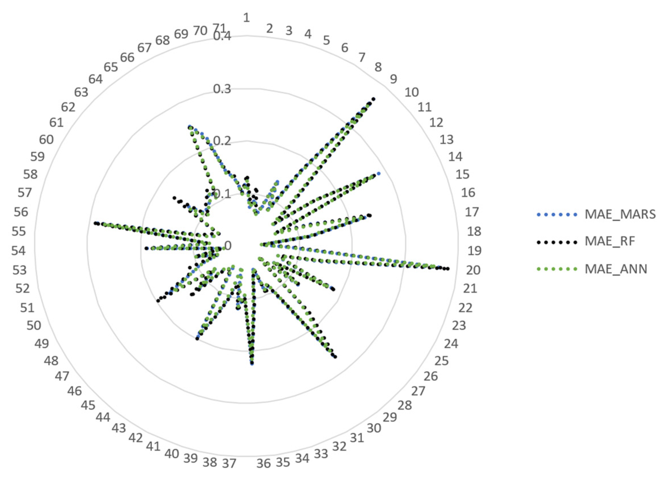
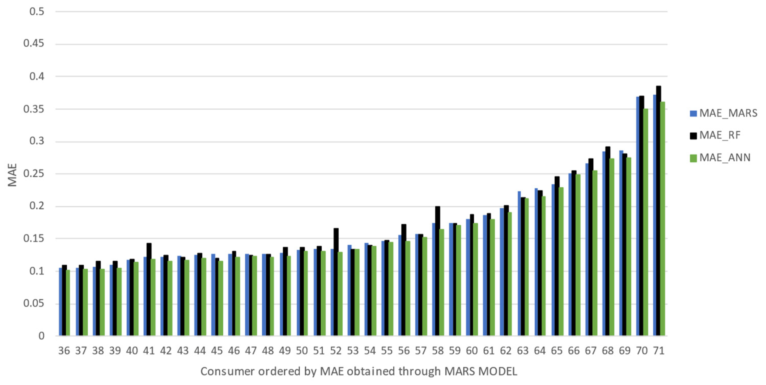
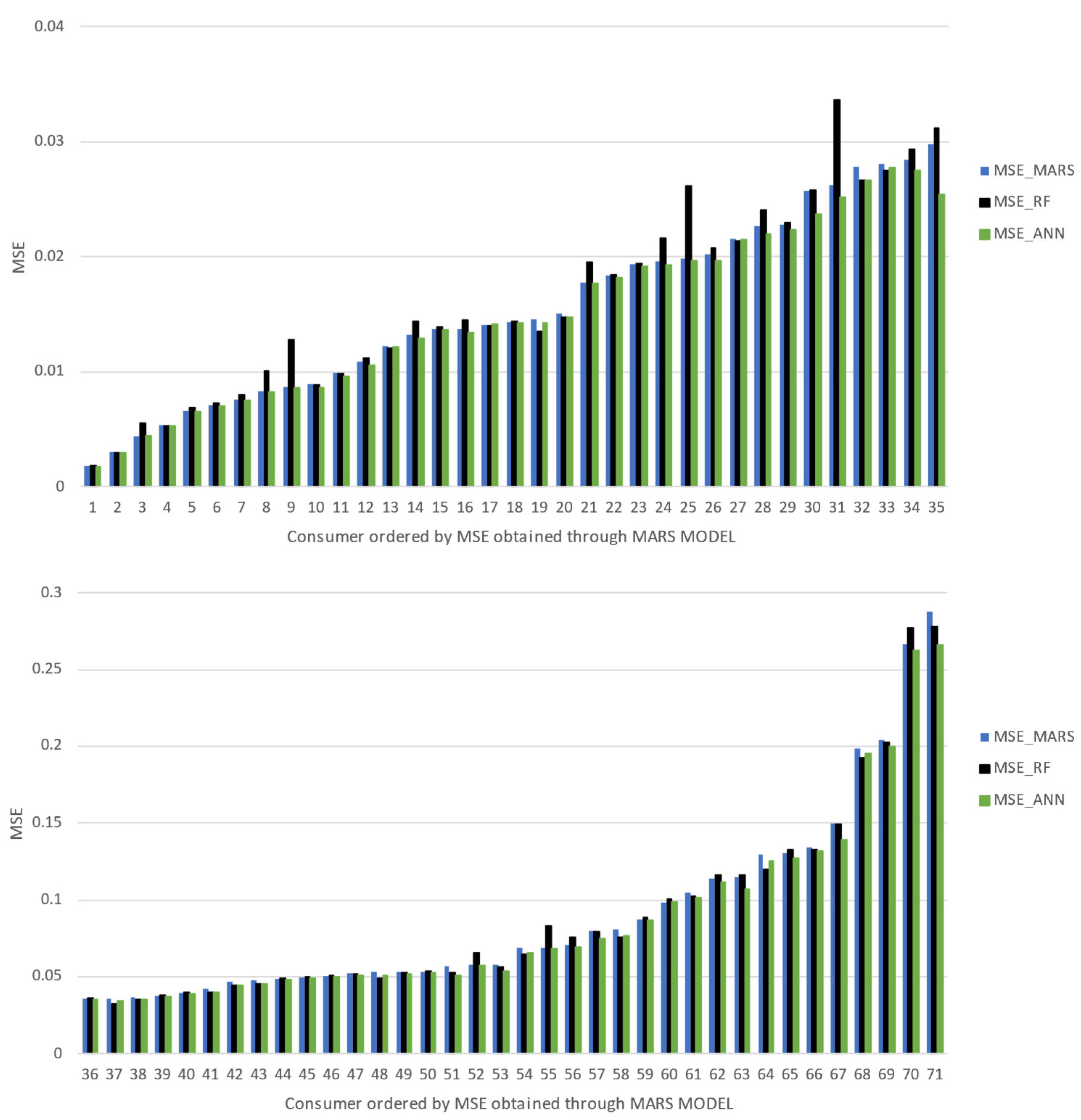
As mentioned earlier, for each one of the 71 consumers, the three different approaches (MARS, RF and ANN) were evaluated and compared with the Naïve model. All the following presented results are related with the test sample. Attending to the MAE metric, it can be stated that ANNs were the most accurate approach for 68 consumers and RF reveals the best performance for the remaining three consumers. In this case, despite MARS models showing similar forecasting performances compared with the concurrent ones, this approach was never the best one. With respect to the MSE metric, ANN was the most accurate approach for 54 consumers, and RF was the most accurate for 16 consumers and the remaining consumer was better forecasted using the MARS model. 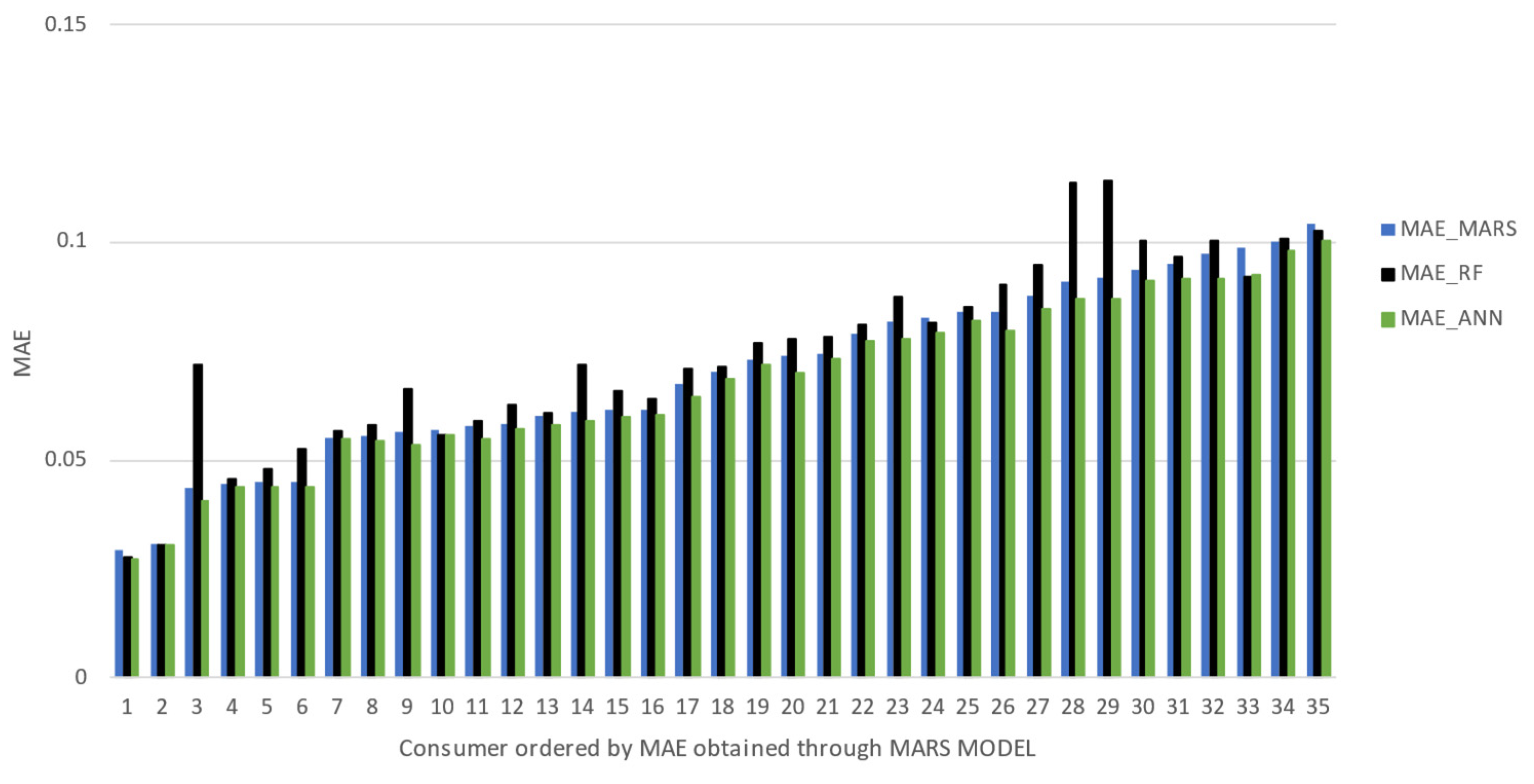The differences in the absolute error metrics are not so significant (as can be visualized in Figure 4 and Figure 5); it is possible to infer that none of the different forecasting approaches applied somehow compromise an expected accuracy range. The radar charts allow a holistic view of the error analysis, with no prior logical order of the different consumers and highlighting the different forecasting methods. However, to allow a clearer analysis, bar charts were also used with an ascending trend of error metrics MAE and MSE, using the MARS model as a reference in the ranking. The bar charts shown in Figure 6 and Figure 7, due to the high number of consumers being involved, were split into two different graphs.

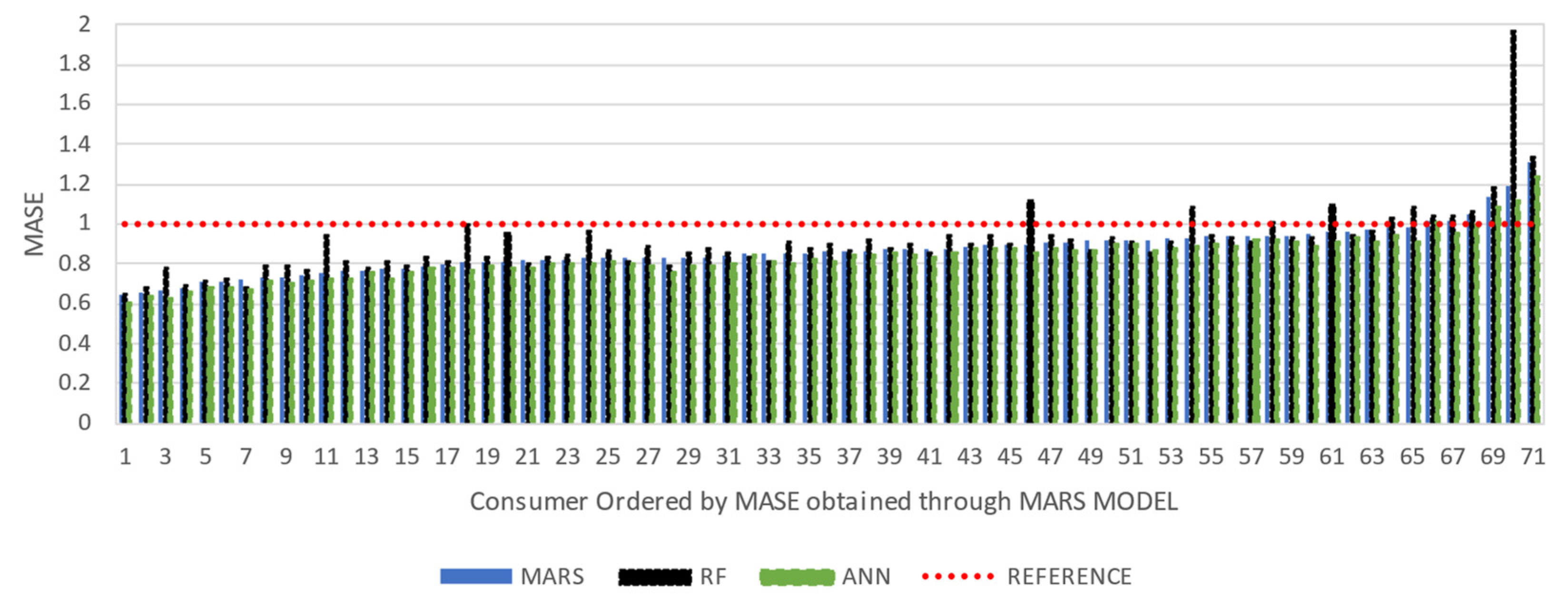
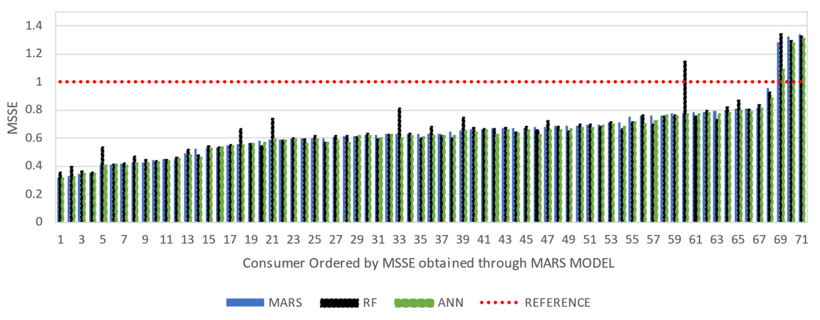
As mentioned earlier, scaled error metrics were also applied using the Naïve model as baseline. A more detailed comparison of different applied models is possible, as shown in Figure 8 and Figure 9. As it is perceived, apart from some residual number of consumers, the forecasting methodologies are more precise than the Naïve model as expected (MASE values are below the unitary value, highlighted as Reference in the chart). For most of the tested consumers, ANN is the most accurate model, but with no significant differences among the approaches. With this MASE analysis, it can be concluded that RF models reveal some weaknesses when applied to some specific consumers. These low performances identified are often related with cases of overfitting, as will be further discussed.

Regarding MSSE analysis, it can be pointed out that for almost all consumers, the three proposed approaches considerably reduce the error metrics identified in the Naïve model (MSSE typically below 0.8).

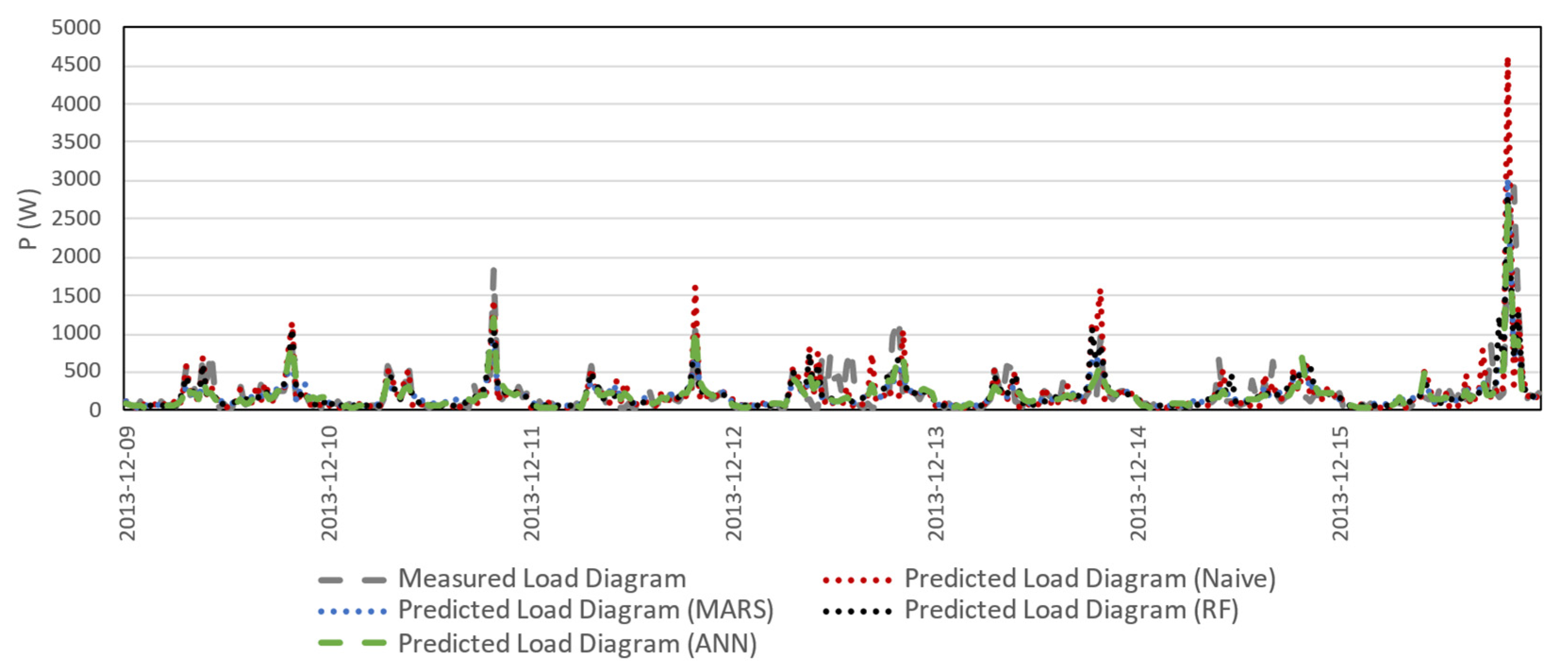
With the perspective of conveying the challenge associated with domestic load forecasting, Figure 10 and Figure 11 present measured weekly load diagrams during the test period and the short-term predictions (day-ahead forecasting) available by using the proposed methodologies. It must be stressed that the electricity consumption records available in the time series were converted to active power to build up these load profiles.

The randomness in resulting active power series is clear and some abrupt changes (sudden peak values or unexpected low values) in active power load are in some cases difficult to predict with the different methodologies. The two presented consumers were chosen due to considerably different consumption volumes as well as load patterns.

3.3. In-Depth Analysis of the Trained Models

With the MARS, RF and ANN models already trained and providing the most accurate predictions for each consumer, it becomes relevant to proceed to a zoom-in look, with the intention of evaluating features’ relevance, training times and also, for the case of ANNs, the networks’ dimension.

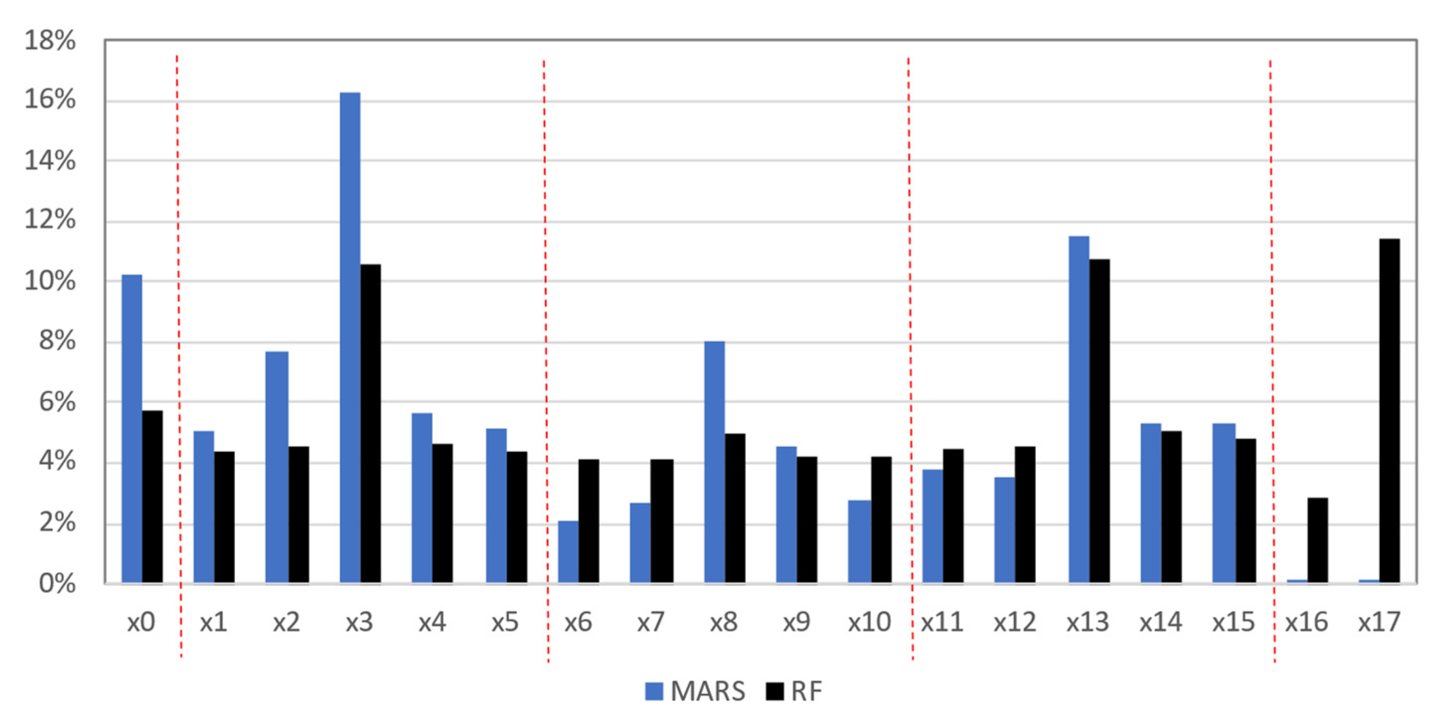
To evaluate features’ relevance in MARS models, the dependence of each model on the different features was identified and, for the different hinge functions and eventual linear dependences of single features, an average of absolute coefficient values was computed. After aggregating the effect verified for the studied consumers, normalised averages (sum of values equal to 1) are presented in Figure 12. The labels are related with the used features (from x₀ to x₁₇) already presented in Table 2. It can be noted that the features x₀, x₃, x₈, and x₁₃ tend to be the most influential in MARS models.

These are related with past record values verified 8 days ago, 7 days ago and 2 days ago at the same hourly period being predicted. The strategy of including “neighbouring” records (not at the similar hourly periods, but at hourly periods hp − 2, hp − 1, hp + 1 and hp + 2) to give the effect of trend when forecasting, denotes specific features (such as x₂, x₁₄ and x₁₅) to be interesting.

In addition, the dependence on the cyclic variables (x₁₆ and x₁₇) seems to be low. With a more detailed analysis, it can be concluded that for the individual models created for each individual consumer, the contribution of these cyclic variables was imposing a linear dependence of these variables without the effect of hinge functions. As the input variables were not normalised, the ranges of these cyclic variables are considerably higher than the historical electricity consumption records (from x₀ to x₁₅); thus, the resulting coefficients are considerably lower, distorting the real effect of these variables.

Proceeding with the same analysis for the RF model and combining the RF features’ relevance for the different models (individual consumers) through an average results in the normalised relevance of each feature, also shown in Figure 12.

It can be validated that the electricity consumption values identified at similar hourly periods 7 days before and 2 days before the day being predicted are the most relevant in the forecasting process. In this case, the cyclic variable associated with the hourly period is also valuable, as the regression trees often create a branch to determine the following sub-node according to this feature.

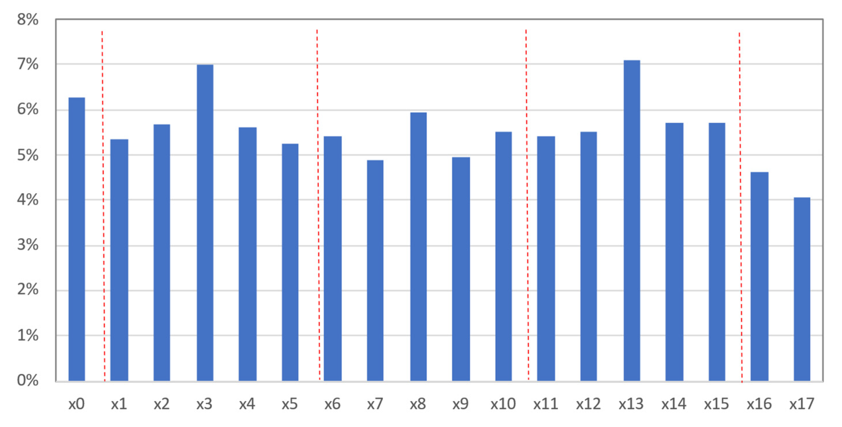
For the interpretation of relevant features in ANN models, after finding the best models, the weights obtained in the first layers (according to the connections between the different inputs and the different neurons assumed in each model) were analysed. For each ANN, an average of the absolute weights associated to each individual feature was assumed to characterise this corresponding feature. At the end, the relative importance of each feature was obtained by an average of its relative importance for the 71 consumers. The resulting normalised relevance for each individual feature is presented in Figure 13.

Again, from the historical electricity consumption data, the electricity consumption records available at the similar hourly periods are the most important. In this case, the relative importance of adjacent hourly periods seems to be more relevant to pass to the ANN, to allow the perspective of transmitting the effect of trend. As before, the effect of day D-7 and day D-2 seems to be more important than that of day D-6. Finally, cyclic variables assume a relative importance in the context of ANN training. In this research, a straightforward analysis to the weights vector in the first layer was followed. Nevertheless, a sensitivity analysis could be followed, involving the concept of partial derivatives, to give a perspective on the local rate of change of the output with respect to an individual input holding the other inputs fixed [27,31]. As the neural network models evaluated use nonlinear activation functions between the different layers, a simple comparison of weights may not be reliable enough. In multilayer networks, a partial derivative has the same interpretation as a weight in a linear model, but instead of extending the analysis to the entire input space, it is only focused on the neighbourhood of the input point being considered.

During different experiments, processing times were recorded for each forecasting model and for each consumer analysed. The PC used during the tests was an Intel-core i7, 2.5 GHz with 12 GB of installed memory (RAM). Despite the available records of training times and simulation times (only during the prediction and not interfering in the modelling) for the training and test subsets, these two latest ones are so negligible that they are not here presented.

Table 3. Training Time Analysis (in seconds).

Model	Min	Average	Max
MARS	0.95 s	10.68 s	79.01 s
RF	40.44 s	83.71 s	1743.81 s
ANN 1	2.30 s	5.45 s	11.54 s

¹ Training times associated with ANN models are related to the most accurate model out of 80 different simulations. (10 trials followed to a variable number of neurons—from 3 to 10).

shows the resulting training times for the different forecasting models.

As can be seen, the most time-consuming is the Random Forest Regressor (RF model), and in some cases (individual consumers) this can be avoided as the models tend to be overfitted. The hyperparameters’ definition would be providential to circumvent this effect. ANN models tend to be rapidly trained; however, several tests were in fact considered, including several trials and different numbers of neurons, until the most accurate model was found. MARS models are a good compromise to have a straightforward and interpretable model, with low computational time to train (not depending on several trials, unless different hyperparameters—maximum number of hinge functions, the penalty parameter or the maximum number of interactions—are explored through a metaheuristic or a grid-search technique).

In Figure 14, it is shown that almost 70% of the consumers tested were in fact modelled with an ANN with seven or more neurons. Despite this fact, error metrics found in ANNs with higher dimensions are not that much lower than the error metrics obtained with lower ANN dimensions. More than the ANN dimension, each energy behaviour idiosyncrasy and the quality of measured data are more influential on the forecasting accuracy, as the forecasting quality was revealed to be not so sensitive to the ANN architecture.

4. Conclusions

The developed research revealed many interesting and useful insights. On one hand, despite the ANN models being more accurate and more flexible to be adapted to different consumers’ patterns, it is clear that the three different forecasting approaches do not differ significantly in accuracy of estimating half-hourly electricity consumption records for the day-ahead, applied to different consumers. This implies that the quality of smart meter data used, the feature selection phase and each model’s parametrization may be quite more determining to enhance the forecasting action, rather than the chosen forecasting model itself. Regarding this, for the electricity supplier/distributor, the trade-off between the accuracy and the interpretability of each individual model must be considered. This conclusion is strengthened when a scale effect is involved, as several individual forecasting models should be trained and used for different end-users.

On the other hand, with a thorough analysis of the trained models, it was possible to identify some relevant features that are transversal to the different approaches (mainly the electricity consumption records measured at similar hourly periods 2 and 7 days before). The strategy of including previous electricity consumption records at hourly periods “adjacent” to the similar hourly periods seems to be more justified in the case of ANN and not so relevant to MARS or RF models. The effects of including cyclic variables to distinguish the consumption pattern specific to each day of the week or even to each hourly period tend to be notorious and should not be avoided. Some experiments were exploited without these cyclic variables, leading to an overall degradation in forecasting performances.

Further research should address the inclusion of exogenous variables in the models (including weather variables on a half-hourly basis or, at least, considering daily meteorological values associated with extreme conditions—e.g., minimum, and maximum values of temperature on a daily basis). To overcome the risk of overfitting in the RF model, different hyperparameters should be explored by eventually using a metaheuristic. Finally, rather than simply looking at the weights vector in the first ANN layer, a sensitivity analysis based on partial derivatives must be followed up to better evaluate features’ relevance in ANNs.

References

1. Wang, Y.; Chen, Q.; Hong, T.; Kang, C. Review of Smart Meter Data Analytics: Applications, Methodologies, and Challenges. IEEE Trans. Smart Grid 2019, 10, 3125–3148. [Google Scholar] [CrossRef]
2. Alberg, D.; Last, M. Short-term load forecasting in smart meters with sliding window-based ARIMA algorithms. Vietnam J. Comput. Sci. 2018, 5, 241–249. [Google Scholar] [CrossRef]
3. Azeem, A.; Ismail, I.; Jameel, S.M.; Romlie, F.; Danyaro, K.U.; Shukla, S. Deterioration of Electrical Load Forecasting Models in a Smart Grid Environment. Sensors 2022, 22, 4363. [Google Scholar] [CrossRef] [PubMed]
4. Albayati, A.; Abdullah, N.F.; Abu-Samah, A.; Mutlag, A.H.; Nordin, R. Smart Grid Data Management in a Heterogeneous Environment with a Hybrid Load Forecasting Model. Appl. Sci. 2021, 11, 9600. [Google Scholar] [CrossRef]
5. Viana, J.; Bessa, R.J.; Sousa, J. Load Forecasting Benchmark for Smart Meter Data. In Proceedings of the 2019 IEEE Milan PowerTech, Milan, Italy, 23–27 June 2019; pp. 1–6. [Google Scholar] [CrossRef]
6. Hayes, B.P.; Gruber, J.K.; Prodanovic, M. Multi-nodal short-term energy forecasting using smart meter data. IET Gener. Transm. Distrib. 2018, 12, 2988–2994. [Google Scholar] [CrossRef]
7. de Mattos Neto, P.S.G.; de Oliveira, J.F.L.; Bassetto, P.; Siqueira, H.V.; Barbosa, L.; Alves, E.P.; Marinho, M.H.N.; Rissi, G.F.; Li, F. Energy Consumption Forecasting for Smart Meters Using Extreme Learning Machine Ensemble. Sensors 2021, 21, 8096. [Google Scholar] [CrossRef]
8. Nti, I.K.; Teimeh, M.; Nyarko-Boateng, O.; Adekoya, A.F. Electricity load forecasting: A systematic review. J. Electr. Syst. Inf. Technol. 2020, 13, 7. [Google Scholar] [CrossRef]
9. Mehdipour Pirbazari, A.; Farmanbar, M.; Chakravorty, A.; Rong, C. Short-Term Load Forecasting Using Smart Meter Data: A Generalization Analysis. Processes 2020, 8, 484. [Google Scholar] [CrossRef]
10. Omitaomu, O.A.; Niu, H. Artificial Intelligence Techniques in Smart Grid: A Survey. Smart Cities 2021, 4, 548–568. [Google Scholar] [CrossRef]
11. Gajowniczek, K.; Ząbkowski, T. Short Term Electricity Forecasting Using Individual Smart Meter Data. Procedia Comput. Sci. 2014, 35, 589–597. [Google Scholar] [CrossRef]
12. Lahouar, A.; Ben Hadj Slama, J. Day-ahead load forecast using random forest and expert input selection. Energy Convers. Manag. 2015, 103, 1040–1051. [Google Scholar] [CrossRef]
13. Yuan, T.-L.; Jiang, D.-S.; Huang, S.-Y.; Hsu, Y.-Y.; Yeh, H.-C.; Huang, M.-N.L.; Lu, C.-N. Recurrent Neural Network Based Short-Term Load Forecast with Spline Bases and Real-Time Adaptation. Appl. Sci. 2021, 11, 5930. [Google Scholar] [CrossRef]
14. Ünal, F.; Almalaq, A.; Ekici, S. A Novel Load Forecasting Approach Based on Smart Meter Data Using Advance Preprocessing and Hybrid Deep Learning. Appl. Sci. 2021, 11, 2742. [Google Scholar] [CrossRef]
15. Lopez-Martin, M.; Sanchez-Esguevillas, A.; Hernandez-Callejo, L.; Arribas, J.I.; Carro, B. Novel Data-Driven Models Applied to Short-Term Electric Load Forecasting. Appl. Sci. 2021, 11, 5708. [Google Scholar] [CrossRef]
16. Kell, A.; McGough, A.S.; Forshaw, M. Segmenting Residential Smart Meter Data for Short-Term Load Forecasting. In Proceedings of the Ninth International Conference on Future Energy Systems (e-Energy’18), Karlsruhe, Germany, 12–15 June 2018; Association for Computing Machinery: New York, NY, USA, 2018; pp. 91–96. [Google Scholar] [CrossRef]
17. Andriopoulos, N.; Magklaras, A.; Birbas, A.; Papalexopoulos, A.; Valouxis, C.; Daskalaki, S.; Birbas, M.; Housos, E.; Papaioannou, G.P. Short Term Electric Load Forecasting Based on Data Transformation and Statistical Machine Learning. Appl. Sci. 2021, 11, 158. [Google Scholar] [CrossRef]
18. Moon, J.; Kim, Y.; Son, M.; Hwang, E. Hybrid Short-Term Load Forecasting Scheme Using Random Forest and Multilayer Perceptron. Energies 2018, 11, 3283. [Google Scholar] [CrossRef]
19. Martinez-Pabon, M.; Eveleigh, T.; Tanju, B. Smart Meter Data Analytics for Optimal Customer Selection in Demand Response Programs. Energy Procedia 2017, 107, 49–59. [Google Scholar] [CrossRef]
20. Almughram, O.; Zafar, B.; Ben Slama, S. Home Energy Management Machine Learning Prediction Algorithms: A Review. In Proceedings of the 2nd International Conference on Industry 4.0 and Artificial Intelligence (ICIAI 2021), Tunisia-Souse, Tunisia, 28–30 November 2021; pp. 40–47, ISBN 978-94-6239-528-2. [Google Scholar] [CrossRef]
21. Massidda, L.; Marrocu, M. Smart Meter Forecasting from One Minute to One Year Horizons. Energies 2018, 11, 3520. [Google Scholar] [CrossRef]
22. Fekri, M.N.; Grolinger, K.; Mir, S. Distributed load forecasting using smart meter data: Federated learning with Recurrent Neural Networks. Int. J. Electr. Power Energy Syst. 2022, 137, 107669. [Google Scholar] [CrossRef]
23. UK Power Networks, Low Carbon London Project. Available online: https://data.london.gov.uk/dataset/smartmeter-energy-use-data-in-london-households (accessed on 27 July 2021).
24. PyEarth Package. Available online: https://contrib.scikit-learn.org/py-earth/ (accessed on 1 September 2022).
25. Ensemble Package. Available online: https://scikit-learn.org/stable/modules/generated/sklearn.ensemble.RandomForestRegressor.html (accessed on 1 September 2022).
26. Hippert, H.S.; Pedreira, C.E.; Souza, R.C. Neural networks for short-term load forecasting: A review and evaluation. IEEE Trans. Power Syst. 2001, 16, 44–55. [Google Scholar] [CrossRef]
27. Sousa, J.C.; Neves, L.P.; Jorge, H.M. Assessing the relevance of load profiling information in electrical load forecasting based on neural network models. Int. J. Electr. Power Energy Syst. 2012, 40, 85–93. [Google Scholar] [CrossRef]
28. Neural Network Package. Available online: https://scikit-learn.org/stable/modules/neural_networks_supervised.html (accessed on 1 September 2022).
29. Energy Follow-Up Survey Report, 2011—Report 1: Summary of Findings, Department of Energy and Climate Change. Available online: https://assets.publishing.service.gov.uk/government/uploads/system/uploads/attachment_data/file/274769/1_Summary_Report.pdf (accessed on 20 June 2022).
30. Cooling in the UK—BEIS—Department for Business Energy and Industrial Strategy. August 2021. Available online: https://assets.publishing.service.gov.uk/government/uploads/system/uploads/attachment_data/file/1019896/cooling-in-uk.pdf (accessed on 20 June 2022).
31. Fidalgo, J.N. Feature subset selection based on ANN sensitivity analysis—A practical study. In Proceedings of the WSES International Conference on Neural Networks and Applications, Tenerife, Spain, 11–15 February 2001; pp. 206–211. [Google Scholar]
Figure 1. Example of a MARS model to approximate a non-linear real function.
Applsci 12 09844 g001
Figure 2. Example of a Random Forest Regressor model (just an example, not corresponding to any decision tree applied during the research).
Applsci 12 09844 g002
Figure 3. Example of a trained ANN model with 5 neurons in the hidden layer.
Applsci 12 09844 g003
Figure 4. Radar chart involving MAE (in kWh) for different Consumer IDs.
Applsci 12 09844 g004
Figure 5. Radar chart involving MSE (in kWh2) for different Consumer IDs.
Applsci 12 09844 g005
Figure 6. Bar charts involving MAE (in kWh) in an ascending order.
Applsci 12 09844 g006aApplsci 12 09844 g006b
Figure 7. Bar charts involving MSE (in kWh2) in an ascending order.
Applsci 12 09844 g007
Figure 8. MASE comparison per consumer ID.
Applsci 12 09844 g008
Figure 9. MSSE comparison per consumer ID.
Applsci 12 09844 g009
Figure 10. First comparison of day-ahead predicted and measured load diagrams (during a week of the test period)—#Consumer 18.
Applsci 12 09844 g010
Figure 11. Second comparison of day-ahead predicted and measured load profiles (during a week of the test period)—#Consumer 59.
Applsci 12 09844 g011
Figure 12. Features’ relevance using MARS and RF models.
Applsci 12 09844 g012
Figure 13. Feature relevance using ANN model.
Applsci 12 09844 g013
Figure 14. ANN Dimensions’ Distribution.
Applsci 12 09844 g014