Article

A Separated-Flow Model for 2-D Viscous Flows around Bluff Bodies Using the Panel Method

1
School of Mechanical Engineering, Lanzhou Jiaotong University, Lanzhou, 730070, China
2
School of Engineering, University of Birmingham, Edgbaston, Birmingham B15 2TT, UK
3
School of Mechanical Engineering, Southwest Jiaotong University, Chengdu 610031, China
*
Author to whom correspondence should be addressed.
Appl. Sci. 2022, 12(19), 9652; https://doi.org/10.3390/app12199652
Submission received: 8 September 2022 / Revised: 19 September 2022 / Accepted: 22 September 2022 / Published: 26 September 2022
(This article belongs to the Special Issue Aerodynamics of High-Speed Trains)

Abstract

:
Panel methods have been applied to many fields of fluid owing to their computational efficiency. However, their applications are limited in simulating highly turbulent flow with separations due to the inviscid flow assumptions, such as those associated with train aerodynamics. Some researchers employed the wake models to simulate large vortices in the wake of trains with predetermined separation locations according to experimental results. In this paper, a modified 2-D constant source/vortex panel method for modelling the separated flow around 2-D bluff bodies is presented. The proposed separated-flow model includes the prediction of separation locations based on the integral boundary-layer method and the shear layer, and large vortices in the wake of the bluff bodies are modelled by the wake model. The proposed method is validated by comparing the calculated pressure distribution on a 2-D circular cylinder with the experimental results. The method is then applied to simulate the flow around a 2-D generic train and calculate the pressure distribution on the train. Since trains run very close to the ground, the effect of the ground configuration on the pressure distribution of the 2-D train is also investigated in this paper using the proposed method. The main contribution of the work is to present a 2-D separated-flow model with wake modelling and separation prediction. The proposed model can be used in the rapid evaluation of bluff-body aerodynamics.

1. Introduction

The aerodynamics of bluff bodies have received extensive attention due to their wide variety of applications, which span from civil engineering to wind engineering, and from bridges to offshore structures, all of which rely heavily on our understanding of bluff-body aerodynamics [1]. Although most of our knowledge of train aerodynamics has been gained via aerospace industrial applications, they essentially fall under the category of aerodynamically bluff bodies [2]. Approaches to investigate the flow around trains can be generalised in the traditional sense into key areas of full-scale experiments, model-scale experiments, and numerical simulations. The latter approach is continuing to increase in popularity for applications in train aerodynamics due to its low cost and the large amount of data that can be generated compared with the experiment methods, especially in relation to full-scale experiments on live railways.
It is well known that simulations using computational fluid dynamics (CFD) methods based on solutions of the full Navier–Stokes equations have provided the ability to understand the overall flow dynamics in much greater detail and jointly with experimental studies can be used in the design and assessment of new rolling stocks. Previous literature on train aerodynamics employs the mesh-based scheme and different turbulence models to simulate the flow around trains [3,4,5]; however, significantly fine meshes are needed in order to capture the features of the thin boundary layer and small-scale eddies, which has led to ever-increasing simulation sizes that are computationally expensive and time consuming [6,7,8,9]. Additionally, these numerical approaches are dependent on the grid quality, especially in high Reynolds numbers [10]. Furthermore, it is particularly computationally expensive and time consuming for simulating certain train operating conditions, such as the modelling of trains in tunnels [11], where the aspect of most concern is the pressure variations induced by the passage of the train.
Although in line with the rapid development of high-performance computers, the computational performance of these methods has been improved, it can still require days, or hours at least, to complete a thorough simulation necessary to understand the key flow characteristics [10]. This current situation conflicts with the increasing demand for accurate, cost-effective tools to predict the aerodynamic behaviour of trains as well as other vehicles and structures [11,12]. Owing to their high efficiency, meshless approaches can be the solutions to the present problems [13,14]. The 3-D CFD simulations based on Navier–Stokes equations can track the flow features inside the tunnel due to the train passage; this method is computationally expensive and demands high-order discretisation schemes to avoid numerical instabilities [15,16]. Owing to the large ratio of the tunnel length to its cross-section diameter, the flow inside the tunnel can be approximated by 1-D equations along the axial axis and solved by the method of characteristics (MOC) [17,18], which provides reasonable results at a lower computational cost in predicting the propagation of the pressure waves inside the tunnels. However, the flow induced by the train at the entry portal of the tunnel is complex and three dimensional, which is hard to simulate using the MOC method, as well as the effects of the geometrical parameters of the tunnel portal and the train on the pressure waves [15,19]. The panel method is an option to model trains in tunnels in two-dimensional (2-D) and three-dimensional (3-D) ways while maintaining lower computational costs at the same time. The authors intend to develop the 2-D model and 3-D model for trains in tunnels, and the first stage of our work is to simulate the flow around the 2-D train. This paper presents a 2-D separated-flow model, including separation prediction and wake modelling, to evaluate the pressure distributions around bluff bodies in high Reynolds number flows. The proposed method is applied to the two-dimensional circular cylinder and the generic train and is mathematically and physically consistent with the real expected physics for the investigated problems.
Based on inviscid incompressible potential flow theory, the panel method is applied to most general geometries by solving linear integral equations over the boundary. The main advantage of the method is to eliminate the need for a computational grid, owing to which it has been considered an appropriate design tool in many fields since the 1960s [20]. The panel method has a broad range of applications in industrial fields including trains. Baker generalised the flow field around a train into four different regions according to the velocities induced by the cruising train: the nose region, the boundary-layer region, the near-wake region, and the far-wake region [21,22]. In the nose region, the flow field for most of the trains is largely inviscid with low turbulence levels; that is, except for extremely blunt trains, where large-scale flow separation occurs. Similar results have been obtained using large eddy simulation (LES) by Hemida et al. [23]. Steinheuer [24] computed the potential flow around train heads with different geometries using a panel method and validated the results with model- and full-scale experiments. Based on the results, a simplified potential flow model, to compute the induced loads on track side objects for an axial symmetric head geometry and cylindrical track side objects, was developed [24]. By simplifying the moving train into a moving point, Sanz-Andres et al. [25,26,27,28], Barrero-Gil and Sanz-Andrés [29], and Rutschmann et al. [30,31] investigated the train-induced effects on track-side infrastructures and head pressure waves using analytical methods. Although analytical models provide satisfactory solutions, they are only applicable after some major geometrical simplifications in the boundary conditions have been made. However, panel methods can be applied to more realistic geometries, and fulfil the boundary conditions on the actual surface [32]. Hermanns et al. [33] and Takei et al. [34] used boundary element methods (panel methods are the application of boundary element methods in fluid dynamics) and the three-dimensional panel method to solve the potential flow around the train nose. Due to the inviscid characteristics of the flow around the train head, potential flow solutions have been applied to predict the pressure variations due to the train passages. Kikuchi et al. [35] performed numerical simulations using the boundary element method to study the pressure changes caused by the train passage and validated the numerical model by comparing with the field test results. Khandhia et al. [36] used the time-stepping low-order panel code, USAERO, based on the solutions of potential flow equations coupled with boundary layer and wake relaxation algorithms to simulate trains passing. The results, based on this method, agreed well with the experimental data in both trends and peak-to-peak pressure changes [36]. Some other researchers developed computing programs based on panel methods. For instance, Johnston et al. [37], Morrow [38], Reinhardt-Piéchowiak and Ducruet [39], and Berenger et al. [40,41] developed their own programs based on panel methods to predict the train-induced pressure loads and head pressure waves when trains pass each other. Their predicted results were tested by means of experiments or numerical simulations and showed good agreements [37,38,39,40,41]. Farhan [42] applied the inviscid three-dimensional source panel method to predict the pressure distributions in the cases of a single train at different yaw angles and a train passing a station or passing another train.
The conventional panel method can only be applied to the potential flows such as the flow in the nose region. Additional models should be considered to simulate the separated-flow regions created by bluff bodies such as trains. Some researchers employed the wake models to perform as the strong large vortices in the wakes. Mahomedali [43] developed a procedure based on the panel method for the calculation of the potential flow around bodies of a circular shape to investigate the flow around the train cross-section. Copley [44,45] proposed a quasi-three-dimensional approach using a 2-D panel method for train cross-section computation and then marching along the train length. He applied this model to the aerodynamic predictions of the train at low incidences. Discrete sources and discrete vortices were adopted to model the body and the wake. It was found that the model failed over the incidence of 50° due to the breakdown of the slender body analogy. Chiu [46,47,48] proposed a separated-flow model for both symmetrical and asymmetrical bluff bodies based on a 2-D second-order vortex panel method, and the computed pressure distribution around the train model and other 2-D bluff bodies agreed very well with the experiments. The model was then updated for the prediction of the aerodynamic loads on an idealised railway train model under crosswind at large yaw angles up to 90°. This model involved a two- and a three-dimensional procedure and employed source and vortex panels to model the surface of the train and the wake on the leeside, respectively, and gave satisfactory results when the flow structure of the wake was mainly of a vortex-shedding type rather than a line-vortex type. Tyll [49] proposed a 2-D vortex panel method and utilised it in the multidisciplinary design optimisation of a magnetically levitated (MAGLEV) train. The model employs a continuous vortex sheet to model the solid surface and discrete vortices to model the shed wake, which better matches the mechanics of the flow and predicts the ground effect flow. Good agreement was shown by comparing the predictions with higher-order computational methods and experimental data.
Therefore, only the flow in the nose region of the train has been accurately simulated using the potential flow theory. In order to simulate the flow and pressure distribution around the train, a wake model is needed to account for the vortices after the rear of the train. In addition, modelling of the wake requires the identification of the flow separation’s locations in advance, which in turn relies on experimental or alternative numerical methods. The locations of the flow separation are determined by the boundary-layer development along the train body, which is a result of the viscous effect and can be predicted using integral boundary-layer methods. In this paper, the separated-flow model is developed to include the viscous and inviscid interaction for predicting the pressure distribution around the 2-D bluff body. In this method, a wake model is employed to simulate the separated flow. The integral boundary-layer method is used to predict the separation position, which includes the approximation of both laminar and turbulent boundary layers as well as the transition in boundary layer. Moreover, an interpolative strategy is used to determine the “correct” wake model and to predict the base pressure. The general analysis procedure of this method consists of a potential flow calculation, a boundary-layer analysis, and a wake model for the separated flow. The entire calculation program is coded up in MATLAB and is validated using experimental data of the flow around a circular cylinder, which is a well-documented highly separated turbulent flow case. The method is then used to predict the pressure distribution along a 2-D train, with and without the ground configuration. The methodology of the present work is introduced in detail in Section 2, including the calculation strategy for potential flow, boundary-layer prediction, and modelling of the separated flow. The method is validated in Section 3 by predicting the separation and pressure distribution around the circular cylinder and comparing the results with the reference data. Then, the proposed model is applied to predict the pressure distribution along a 2-D generic train with and without ground configuration. The conclusions of the findings in this work and the advantages and disadvantages of the present model are presented in Section 4.

2. Methods

This work mainly deals with the flow around the bluff bodies. In general, the maximum operational speed of a train is no more than 350km/h, which can be classified as a subsonic flow. Thus, the effect of compressibility is neglected here as the Mach number of the investigated problems in this paper is under 0.3. However, this is not the case for trains running in a tunnel, where the compressibility effect cannot be ignored [10]. The proposed model will be modified and improved dealing with this problem hereafter. In this paper, only the flow around the trains will be considered and thus the compressibility effect is not included.
The calculation procedure of the methodology presented in the current paper is shown in Figure 1. The procedure begins with the coordinates of discretised geometry in panel form as an input. The inviscid flow field around this configuration is then simulated by the potential flow method. The integral boundary-layer method is then used to predict the separation locations for the bluff body based on inviscid velocities obtained from the potential flow calculation in order to model the separated flow. The calculated edge velocities are then used to correct the right-hand side of the potential flow simulation matrix by adding them into the streamwise freestream velocities. The calculated separation locations, where the vorticity shear layer leaves the surface of the bluff body, together with the calculated “correct” wake length map the separated-flow region of the bluff body. Eventually, the velocity and pressure fields are updated by a new potential flow calculation with the separated-flow model. With the updated velocity field, the boundary-layer calculation is made again to find the new separation positions. The iterative procedure continues until the predicted separation positions coincide with the last calculation. The predicted pressure field for the entire body in both attached and separated flow results from this procedure.

2.1. Potential Flow Calculation

The potential flow around the body is computed using the 2-D constant source panel method, as described in detail in Katz and Plotkin [32], Chiu [46], and Dvorak [50]. The incompressible flow field around an arbitrary shape is governed by mass and momentum conservation equations. With the inviscid irrotational potential flow assumption, the mass conservation equation is simplified to the Laplace equation in terms of the velocity potential Φ and governs the potential flow independently:
2 Φ = 0 ,
The pressure field is calculated using the momentum equation (Bernoulli equation). Thus, the problem is to solve Laplace’s equation for one unknown scalar, which is a linear problem. For the exterior flow case, the flow should be bounded by the solid surface of the arbitrary body and no penetration is allowed through the body surface. In the present work, the Neumann boundary condition, which is imposed on the Laplace equation and specifies the values of the derivative applied at the boundary of the domain, is selected to specify a zero normal velocity component on the boundary surface directly:
Φ ·   n = 0 ,
where n is the unit normal vector in the out-of-plane direction. The configuration surface is approximated by n straight-line panels, and each panel has a control point, normally taken as the midpoint, where the boundary conditions are applied. The perturbation velocity fields, u and v, at point P (x,y) included by a panel with coordinates (x1,y1) and (x2,y2) and constant source strength σ is calculated as follows:
u = σ 4 π ln ( x x 1 ) 2 + ( y y 1 ) 2 ( x x 2 ) 2 + ( y y 2 ) 2 ,
v =   σ 2 π ( tan 1 y y 2 x x 2 tan 1 y y 1 x x 1 ) ,
The boundary condition is satisfied if the normal velocities of all of the control points on the panels are equal to zero. Thus, a system of linear equations is constructed and the constant source strength of each panel is obtained by solving the system:
[ A i j ] { σ j } = { RHS i } , A i j = ( u , v ) i j ·   n i , RHS i = ( U , V ) ·   n i ,
where Aij is the matrix of aerodynamic influence coefficients referring to the normal velocity at the i-th control point induced by the j-th panel, σj is the constant source strength of the j-th panel, RHSi is the right-hand side term, which is equal to the normal velocity due to the freestream velocity (U,V) at the i-th control point, and ni is the normal vector of the i-th panel.
The matrix is solved here by the Gaussian elimination method and the velocity and pressure at any point in the flow field can be calculated using the calculated constant source strength. According to the Bernoulli equation, the pressure distribution is computed using the total tangential velocity at each control point by Equation (6).
C p i = p p 1 2 ρ Q 2 = 1 2 ρ ( Q t i 2 Q 2 ) 1 2 ρ Q 2 = 1 Q t i 2 Q 2       ,   Q t i = ( j = 1 N ( u , v ) i j + ( U , V ) ) ·   t i ,
where C p i is the pressure coefficient of the i-th control point, Q t i is the total tangential velocity magnitude at the i-th control point, which is 0 at the stagnation point, and C p i = 1 . Q is the freestream velocity magnitude and ti is the unit tangential vector of the i-th panel.

2.2. Boundary-Layer Prediction

The separated flow can be calculated with the separated-flow model [46,47,48,50]. The separated shear layers of the bluff body are represented by two vortex panels for which strength is calculated using the panel method. However, the separation positions should be prescribed according to experimental results or high-fidelity numerical simulations. Both measures are costly and time consuming. Thus, the separation positions are normally considered as unknowns for design problems that need to be economic both in terms of expense and time. To tackle this, the boundary-layer integral methods are used as an alternative approach in this work, which are relatively simple and fast in predicting the boundary-layer characteristics [51,52,53,54,55]. To represent flows with limited separation regions accurately, viscous equations should be adopted in the present work. Compatibility between laminar and turbulent formulations is necessary to represent the transition in a well-ordered and analytically continuous manner. The fewest additional variables related to viscosity should be added to the global Newton solution procedure for solving the boundary-layer parameters to ensure the computational efficiency.
The two-equation integral formulation [51,52,55] based on dissipation closure is suitable for developing the numerical model. The transition is predicted by spatial amplification theory [56,57] together with an extra lag equation [58,59]. Compared to one-equation methods, such as Thwaites’ method [54], two-equation methods possess the capability of describing thin separated regions and are suitable for the development of the proposed model.
The formulations to represent the incompressible boundary layer in this work employ standard integral momentum and kinetic energy shape parameter equations, based on the formulations presented in Drela and Giles [52] with slight modifications for incompressible flow applications [60]:
d θ d ξ + ( 2 + H ) θ u e d u e d ξ = C f 2 ,
θ d H * d ξ + H * ( 1 H ) θ u e d u e d ξ = 2 C D H * C f 2 ,
where ξ is the streamwise coordinate, and ue is the streamwise potential flow velocity at the edge of the boundary layer. The remaining five parameters, θ, H, H*, Cf, and CD, in the two equations are unknowns, which are the boundary-layer momentum thickness, the shape parameter, the kinetic energy shape parameter, the skin friction coefficient, and the dissipation coefficient, respectively. Thus, additional functional dependencies must be assumed to close the integral boundary-layer equations. For the incompressible laminar flow, the relationships are approximated based on the Falkner–Skan one-parameter profile family and the expressions of H*, Cf, and CD in terms of θ, H, and momentum thickness Reynolds number Reθ are presented as follows:
H * = { 1.515 + 0.076 ( H 4 ) 2 H ,   H < 4 1.515 + 0.040 ( H 4 ) 2 H ,   H > 4 ,
R e θ C f 2 = { 0.066 + 0.066 ( 6.2 H ) 1.5 H 1 ,   H < 6.2 0.066 + 0.066 ( H 6.2 ) 2 ( H 4 ) 2 ,   H > 6.2 ,
R e θ 2 C D H * = { 0.207 + 0.00205 ( 4 H ) 5.5 ,   H < 4 0.207 0.100 ( H 4 ) 2 H 2 ,   H > 4 ,
For the incompressible turbulent flow, closure functions for Cf and H* are obtained from the Coles out-layer profile. The Coles skin friction formula is used as the closure correlation for Cf:
C f = 0.3 e 1.33 H ( log 10 R e θ ) 1.74 + 0.31 H ,
and H* is approximated by the following formula:
H * = { 1.505 + 4 R e θ + ( 0.165 1.6 R e θ 1 / 2 ) ( H 0 H ) 1.6 H ,   H < H 0 1.505 + 4 R e θ + ( 0.04 H + 0.007 ln R e θ H H 0 + 4 / ln R e θ ) ( H H 0 ) 2 ,   H > H 0 ,
where H 0 = min ( 3 + 400 R e θ , 4 ) .
However, the Coles out-layer profile is not sufficient to obtain the remaining closure for CD because this parameter also depends on the Reynolds stresses. Based on the characteristics of equilibrium turbulent flows, the dissipation coefficient CD can be approximated by a sum of the wall layer and the wake layer contribution:
C D = C f 2 U s + C τ ( 1 U s ) ,
U s = H * 2 + ( 1 H 1 0.75 H ) ,
where Us is the effective slip velocity and Cτ is the wake-layer shear stress coefficient. This closure introduces a new variable, Cτ, and according to previous research [52,58,59], this parameter is governed by Green’s lag entrainment equation [58]:
δ C τ d C τ d ξ = 5.6 ( C τ eq 1 / 2 C τ 1 / 2 ) + 2 ( δ u e d u e d ξ ) eq 2 δ u e d u e d ξ ,
C τ eq = 0.015 H * 1 U s ( H 1 H ) 3 ,
( δ u e d u e d ξ ) eq = δ / θ 0.75 H [ C f 2 1 44.89 ( H 1 H ) 2 ] ,
δ = ( 3.15 + 1.72 H 1 ) θ + H θ ,
where δ is the boundary-layer thickness, and the subscript ‘eq’ refers to the equilibrium state.
The envelope method is used in the present work [52,56,57] for the boundary-layer transition, which assumes that the transition occurs when the most unstable Tollmien–Schlichting wave in the boundary layer has grown by some factor, usually taken to be e9. The logarithm of the maximum amplification rate n ¯ with respect to the streamwise coordinate ξ is expressed as a function of H and θ:
θ d n ¯ d ξ = { 0 ,   R e θ < R e θ 0 = 1 θ d n ¯ d R e θ ( θ d R e θ d ξ ) , R e θ > R e θ 0 ,
d n ¯ d R e θ = 0.028 ( H 1 ) 0.0345 exp [ ( 3.87 H 1 2.52 ) 2 ] ,
θ d R e θ d ξ = 0.05 + 2.7 H 1 5.5 ( H 1 ) 2 + 3 ( H 1 ) 3 + 0.1 exp ( 20 H 1 ) ,
log 10 R e θ 0 = 2.492 ( H 1 ) 0.43 + 0.7 [ t a n h ( 14 H 1 9.24 ) + 1 ] ,
The entire boundary-layer region is divided into a laminar interval and a turbulent interval, separated by a transition location   ξ t r . The momentum equation and the shape parameter equation are solved for the entire boundary layer. The amplification equation is solved for the laminar interval, while the lag equation is solved for the turbulent interval. The transition onset location ξ t r does not have to be on one of the edge points—it can be solved implicitly by the interpolation of its neighbour. Weighted averages of the laminar and turbulent subintervals are the actual governing equations of the transition interval. To define the development of the turbulence based on the onset location, Drela and Giles [52] suggested using 0.7 times its equilibrium value as the initial value of C τ at   ξ t r . In this work, the boundary layer is calculated in MATLAB and the the fsolve function is used to solve the system of nonlinear equations.
The effect of boundary-layer displacement on the potential flow is simulated by distributing sources of known strength on the panels used to describe the geometry. The strengths of these sources are determined directly from the boundary-layer solutions as:
q i = d ( u e i δ * i ) d ξ ,
where u e i is the streamwise potential flow velocity at the edge of the boundary layer and δ * i is the streamwise displacement thickness. The addition of the source distribution modifies the normal velocity at the control point of the i-th panel. Consequently, Equation (5) is modified as:
[ A i j ] { σ j } = { RHS i q i } ,
As the original geometry is not modified using distributed sources, the aerodynamic influence coefficient matrix need not be recalculated. Subsequent iterations between the potential flow and boundary-layer calculations result in convergent solutions.

2.3. Separated-Flow Model

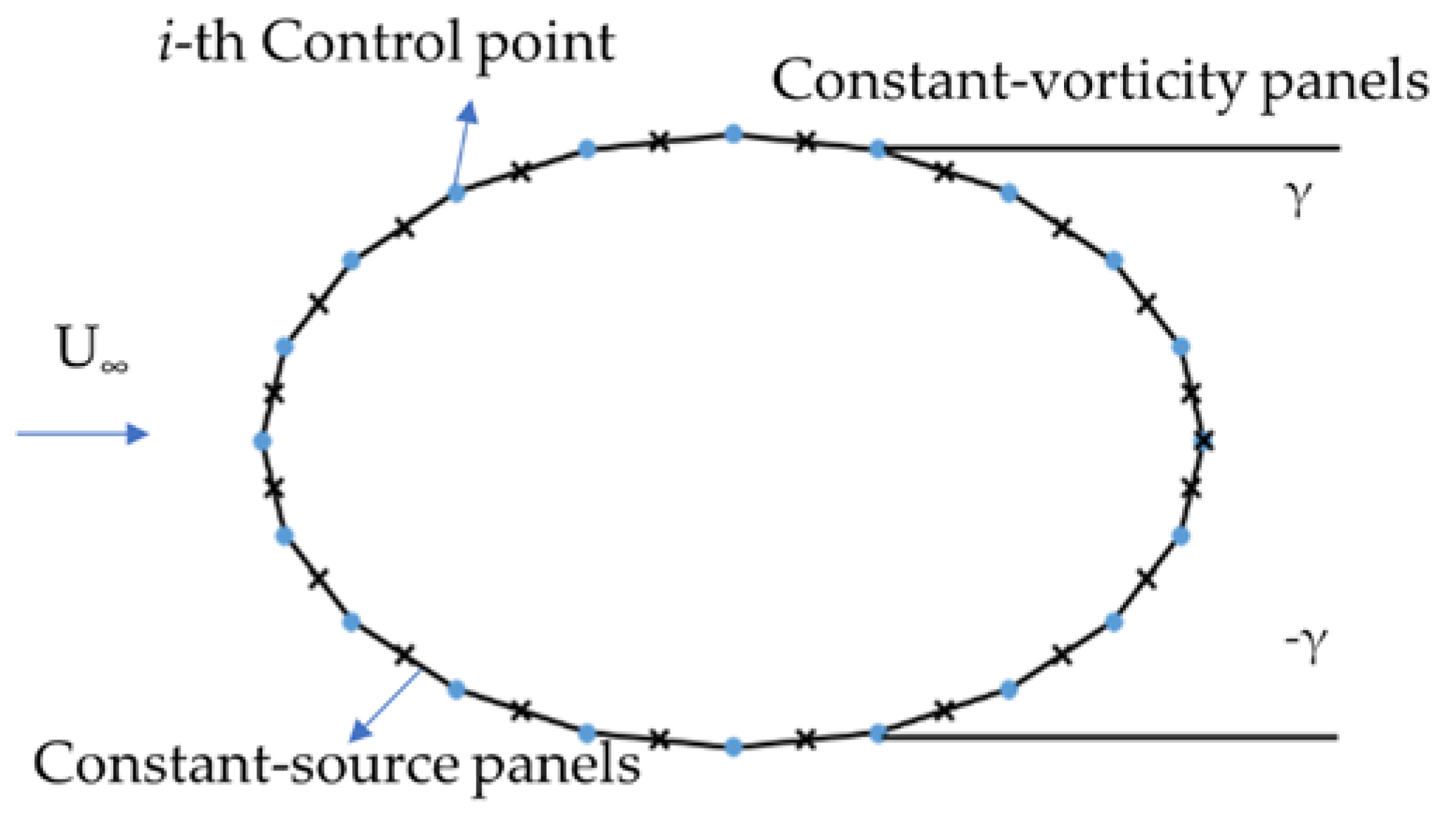
The flow field around a body with separation can be identified as four regions: the potential flow region, the boundary layer, the free shear layer, and the wake. In the panel method, a simplified theoretical model of the real flow is shown in Figure 2: the body is represented by a number of constant source panels and the free shear layers emerging from the separation points of the body are represented by constant vortex panels. The wake panels are attached to the body at the body panel edges nearest to the separation point. One thing worth noting is that the time-varying wake in real flow is represented by two steady vortex sheets, so the flow characteristics calculated are thus time averaged values.
There are normally two vortex sheets forming the wake behind a 2-D bluff body. In the steady model, we should have the same loss of total head across the two vortex sheets. Therefore, the vorticity values of the two vortex sheets have to be equal in magnitude and opposite in sign. This separation model is the same with the model in Dvorak’s work [50]. In addition to the constant source panels on the body surface, a constant vortex distribution γ is assumed on the wake panels. The perturbation velocity induced by the constant vortex panel is different from Equations (3) and (4):
u = γ 2 π ( tan 1 y y 2 x x 2 tan 1 y y 1 x x 1 ) ,
v = γ 4 π ln ( x x 2 ) 2 + ( y y 2 ) 2 ( x x 1 ) 2 + ( y y 1 ) 2 ,
Equation (25) is modified as:
[ A i j ] { σ j } + { B i k } { γ k } = { RHS i q i } ,
where i is the index number of control points including the ones on the wake panel, j is the index number of panels on the body surface, and k is the index number of wake panels, which are up to two in the case of flow around bluff bodies. Aij is the matrix of aerodynamic influence coefficients referring to the normal velocity at the i-th control point induced by the j-th panel, σj is the constant source strength of j-th panel, and Bik is the matrix of the normal velocity at the i-th control point induced by the k-th wake panel with constant vorticity strength γk.
In the separated-flow region, the pressure coefficient in the base flow region is practically constant. This is taken as the base pressure coefficient. The base pressure coefficients within the separated-flow region are calculated as:
C p b = 1 ( Q t i Q ) 2 ( γ s Q ) 2 ,
where Cpb is the corrected surface pressure coefficient in the recirculation region where the velocity of the i-th panel is Q t i , and γs is the vorticity of the shear layer.
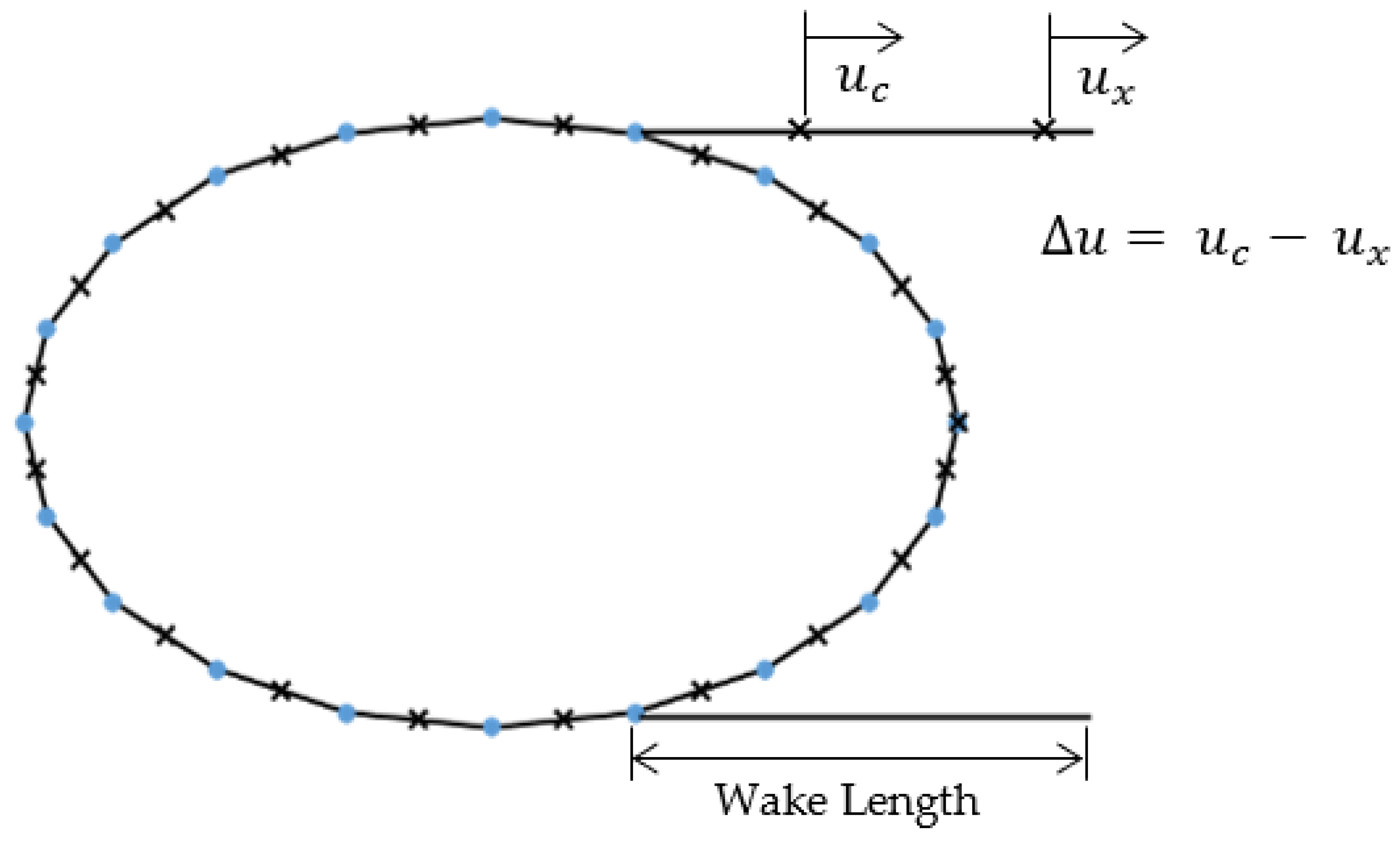
Base pressure coefficients are sensitive to the length of the wake panels. Dvorak [50] and Chiu [46] investigated the relationships between the wake panel lengths and the base pressure coefficients in a 2-D circular cylinder case. They observed that the shorter wake length gave good agreement with experimental pressure over the whole cylinder rather than the longer wake panels, which tend to underestimate the peak suction upstream of the separation. The essentiality of the “correct” wake in predicting the pressure distribution around the bluff body is self-evident due to the separation of the flow. As the “correct” wake length is not known a priori, researchers try to find ways to obtain it. Chiu [46] used experimental base pressure coefficients to obtain the correct wake length. However, this method is difficult to implement in the absence of experimental data. Dvorak [50] provided several solutions to this problem. The first solution is to combine the constant pressure criterion with a multiple segment vortex panel. This requires additional control points and equations. However, this approach is not general enough for application to other shapes. The second solution uses the criterion of zero tangential velocity difference between two points on the wake panel, in an iterative way. Evaluating the tangential velocity increment for two wake length assumptions enables a wake length to be interpolated, which gives a zero-velocity increment, as shown in Figure 3.

3. Results

3.1. Flow Past the Cylinder

To validate the present separated-flow model and the prediction of the separation locations, the simulations for the viscous flows over a 2-D circular cylinder at high Reynolds numbers (Re) have been carried out using the developed method. The results of the present model are verified and validated using the simulation and experiment results of previous studies from the literature [50,61].
In the separated-flow model, the body is represented by a certain number of constant-source panels and the free shear layers by uniform vorticity panels aligned in the free-stream direction, attached to the body at the source panel edges nearest to the separation points. The flow field simulated using the presented model is shown in Figure 4a. For bodies with symmetrical axes parallel to the freestream, the two wake panels will have the same length, and the separation positions on the upper and lower surface are the same. The separation points are predicted by boundary-layer calculations, and the wake lengths, which are highly relevant to the base pressure, are determined by the solution proposed by Dvorak [50]. Roshko’s experiment of flows around the circular cylinder at Re = 8.4 × 10⁶ [61] are used to validate the proposed model. The separation angle predicted by the boundary-layer calculation is 105° for Re = 1 × 10⁷, which coincides with the experimental results. The pressure distribution on half the cylinder of this case is compared with potential flow results, Dvorak’s [50] simulations results, and Roshko’s experimental results [61], as shown in Figure 4b. One thing worth mentioning is that the present method corrects the pressure coefficient at the separation positions by assuming the velocity there is zero. This resolves the “overshoot” in pressure just upstream of the separation point in Dvorak’s results [50]. The independence of the pressure distribution on panel densities is validated by comparing the results of the 40-Panel case and 120-Panel case. Both simulations agree well with the experimental results.
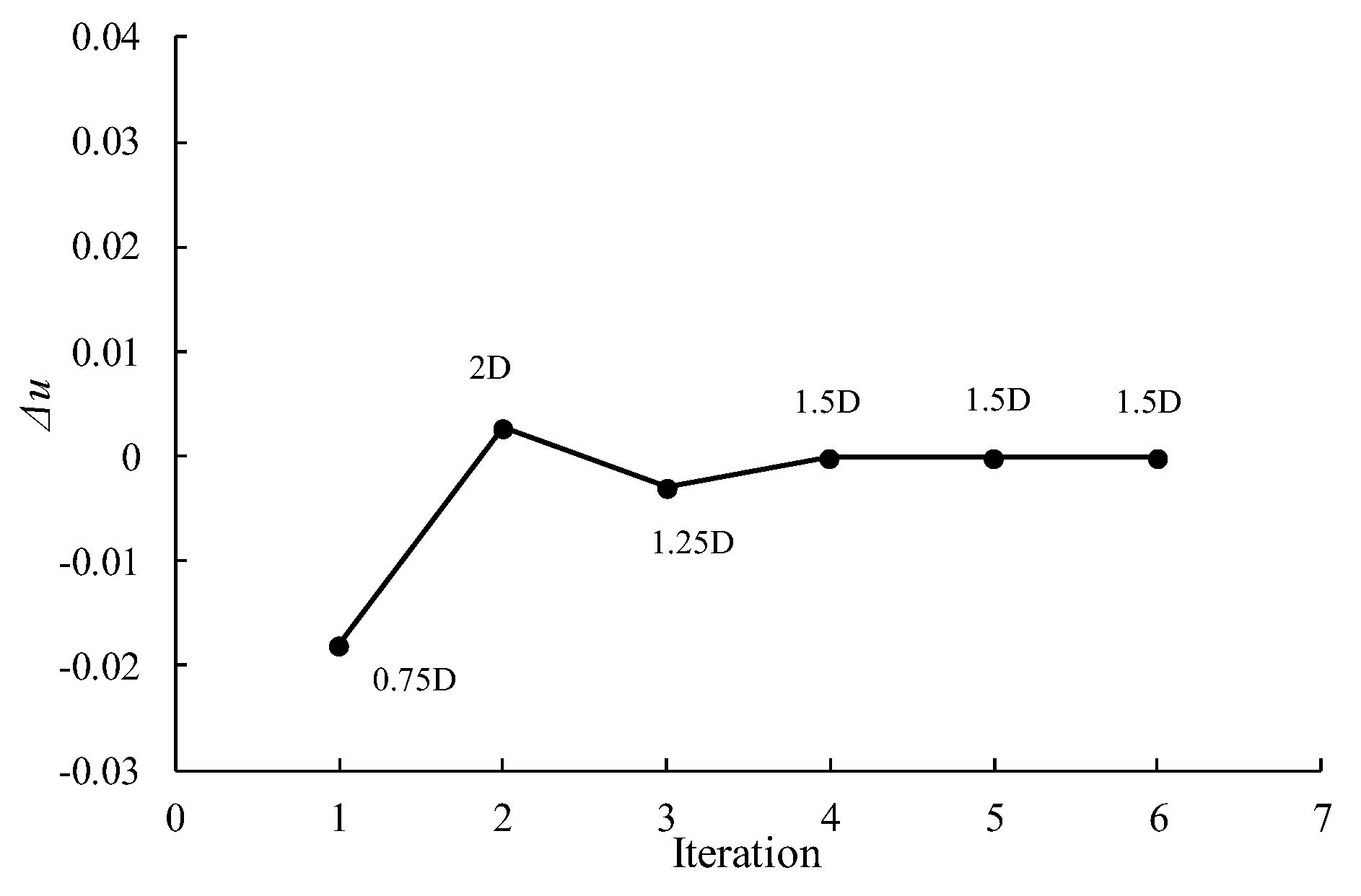
In order to determine the “correct” wake length, the distributions of the tangential velocity increment calculated according to Figure 3 on a circular cylinder with various wake lengths are studied, as shown in Figure 5. The tangential velocities along the wake panels with lengths ranging from 0.75D to 1.5D are investigated, where D refers to the diameter of the 2-D circular cylinder. It is shown that the shorter the wake panel, the larger the increment. For longer wake panels, the tangential velocity first decreases slightly and then increases along the wake panels. Evaluating the tangential velocity increment for two wake length assumptions enables a wake length to be interpolated, which gives a zero-velocity increment. The iteration process shown in Figure 6 starts with two assumed wake lengths, 0.75D and 2D, and it is converged after three iterations to 1.5D. This validates that the proposed interpolative procedure can be used to determine the “correct” wake length for the 2-D bluff bodies in evaluating their pressure distributions using the presented separated-flow model.

3.2. Flow Past the Train

The present method is used to predict the pressure distribution along a 2-D train surface to validate its adaptivity to the flows around the trains. The influence of the presence of the ground is investigated as well.

3.2.1. Physical Model

The 2-D generic train proposed by Chiu and Squire [62] is employed here due to its simplicity, generic shape, and the availability of experimental and numerical data that can be used for validation. The cross-sectional profile of the generic train model is defined by the following equation:
| y | n + | z | n = c n ,
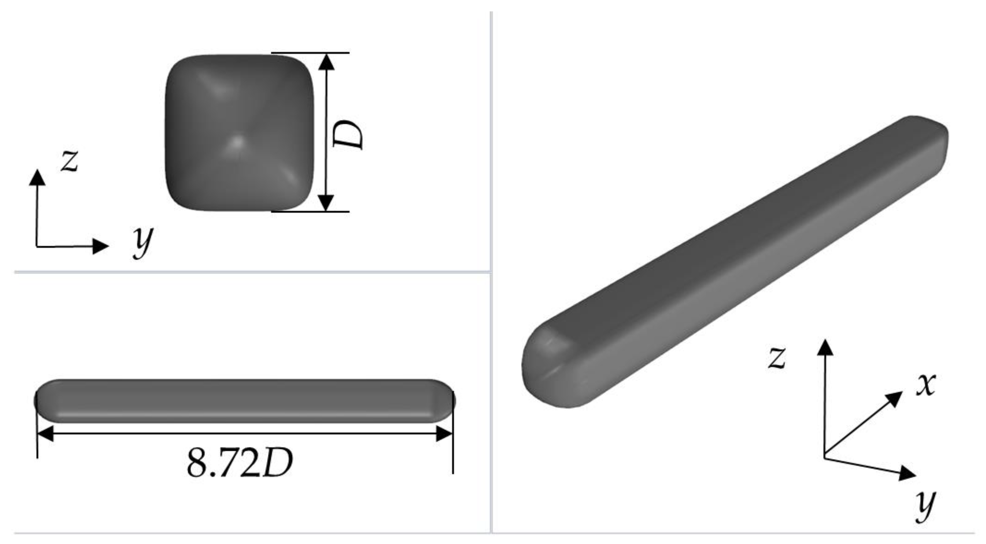
where y and z refer to the vertical and horizontal directions, respectively. The model consists of two parts: a train body and a nose. The train body is of a cylindrical shape with a height Dtr = 125 mm and a total length of 8.72 Dtr, which is in 1:32 scale to the real train. The cross-section profile follows the above equation in which the value of c = 62.5 mm (Dtr/2) and n = 5. The nose cross-section is given by the same equation in which c follows a semi-elliptical profile with a major diameter of 1.28 Dtr, while n is reduced uniformly to 2 at the nose tip. In this way, the cross-section becomes smaller and more circular toward the nose, as shown in Figure 7. The 2-D train model is discretised evenly in the following cases. The Reynolds number is 3 × 10⁵ in the following simulations.

3.2.2. Pressure Loads on the Train

The present separated flow model based on the panel method is used to predict the pressure distribution on the 2-D generic train at the Reynolds number of 3 × 10⁵. The calculation procedure follows the flowchart shown in Figure 1. As explained above, the separated flow model for simulating the viscous flow has two key parameters: the separation locations at which the vorticity panels are attached, and the “correct” wake panels with which the wake is modelled. In the former key parameter, separation locations are predicted by the boundary-layer calculation procedure as described in Section 2.2. The latter key parameter, the “correct” wake panel lengths, are calculated according to the interpolating procedure based on the criterion of zero tangential velocity increment between two points on the wake panels.
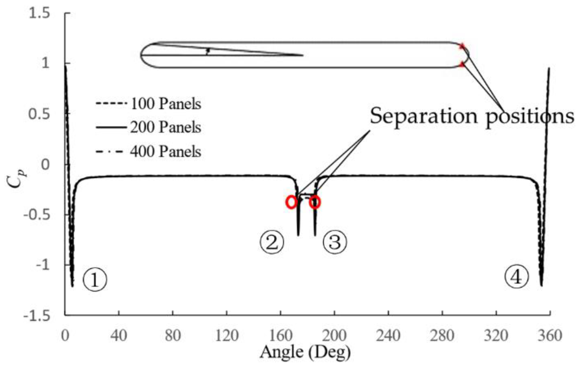
The 2-D generic train has a blunt nose in both the front and the rear part of it, and as the air flows around the train, it tends to separate when reaching the rear part of the train. Figure 8 shows the pressure coefficient along the 2-D train surface using the separated-flow model. The separation positions predicted by the integral boundary-layer method are about 176° on the upper surface and 184° on the lower surface of the train, as shown in Figure 9.
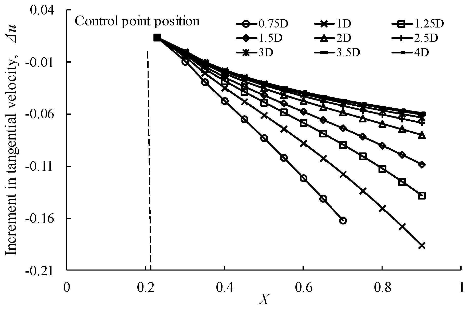
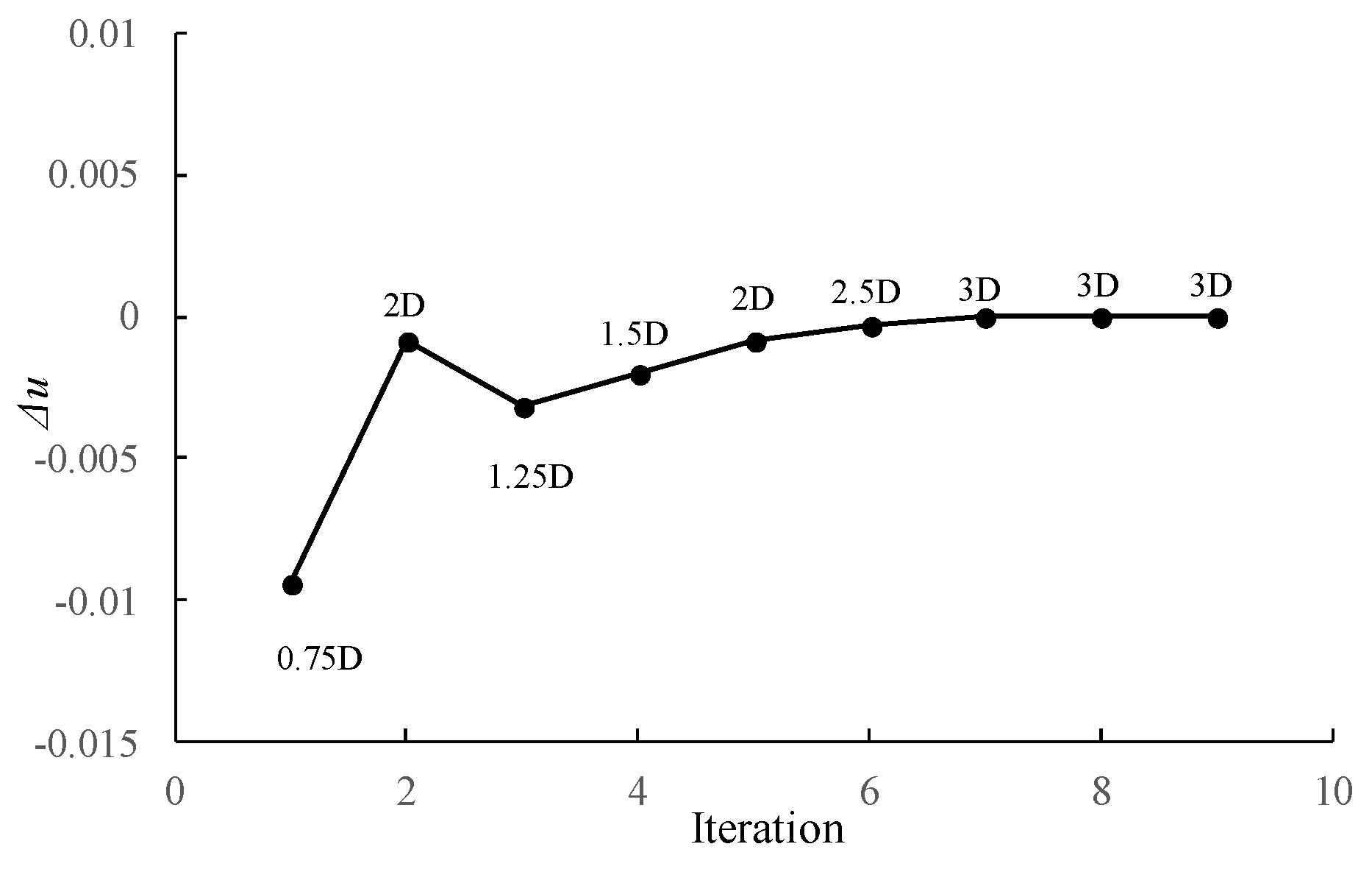
Like the symmetrical simulation of the cylinder flow above, the generic train is geometrically symmetric and the lengths of the wake panels should be the same on the upper surface and lower surface of the train. The distributions of the tangential velocity increment on the wake panels of the train with wake lengths vary from 0.75 Dtr to 4 Dtr are investigated, as shown in Figure 8. For all wake lengths, the tangential velocity increases along the wake panels. The increments in tangential velocity for the wake panels decreases with the increasing of the wake panel lengths; in other words, longer wake panels lead to smaller tangential velocity differences. The “correct” wake panel lengths were determined by the interpolative procedure elaborated in Section 2.3 and validated in Section 3.1. The iteration process shown in Figure 10 starts with two assumed wake lengths, 0.75 Dtr and 2 Dtr, and it is converged after six iterations to 3 Dtr, which is used as the “correct” wake length in evaluating the pressure distribution around the 2-D train. To validate the grid independency of the proposed model, three different panel densities: 100 panels, 200 panels, and 400 panels were tested, as shown in Figure 9. It can be seen that the distribution and value of the pressure coefficient almost coincide for all three cases. The peak values and base pressure are compared in Table 1. The discrepancies of peak values between different panel densities are mainly caused by the locations of the control points and it can be concluded that the differences between the results of 100 panels and 200 panels are small. Thus, the results of the proposed model are independent of the panel densities.
The pressure coefficient is distributed almost symmetrically on the upper surface and the lower surface of the 2-D train. When the flow encounters the train, the stagnation point appears where the pressure coefficient is the maximum. As the flow passes the train head, the pressure decreases rapidly to the minimum, and then increases until the flow reaches the body of the train. The pressure along the train body remains constant and then drops where the body transits to the tail. When separation occurs, the pressure rises and remains constant in between two separation locations on the upper and lower surface, where the pressure is referred to as the base pressure. The base pressure of the 2-D train predicted by the present separated-flow model using 200 panels is −0.3.
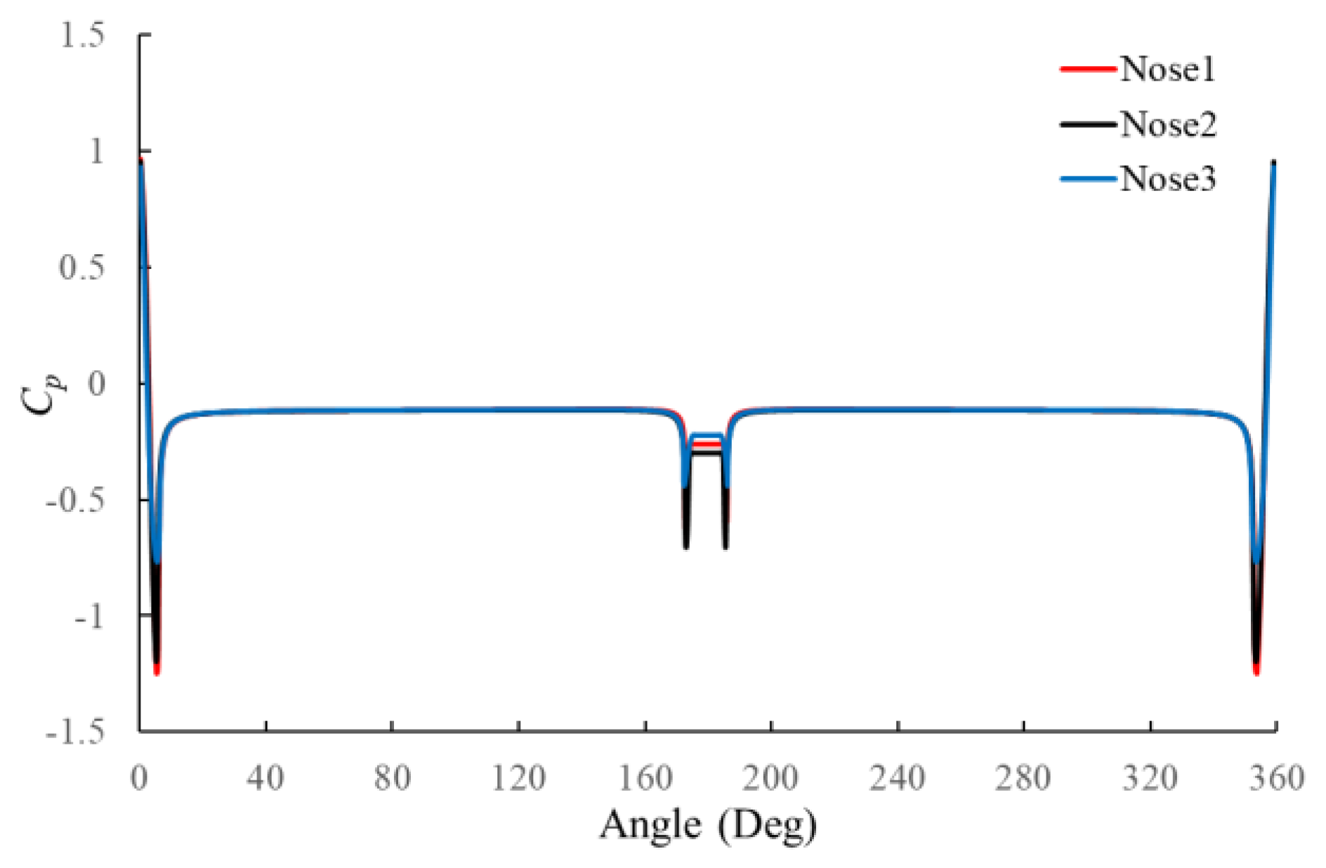
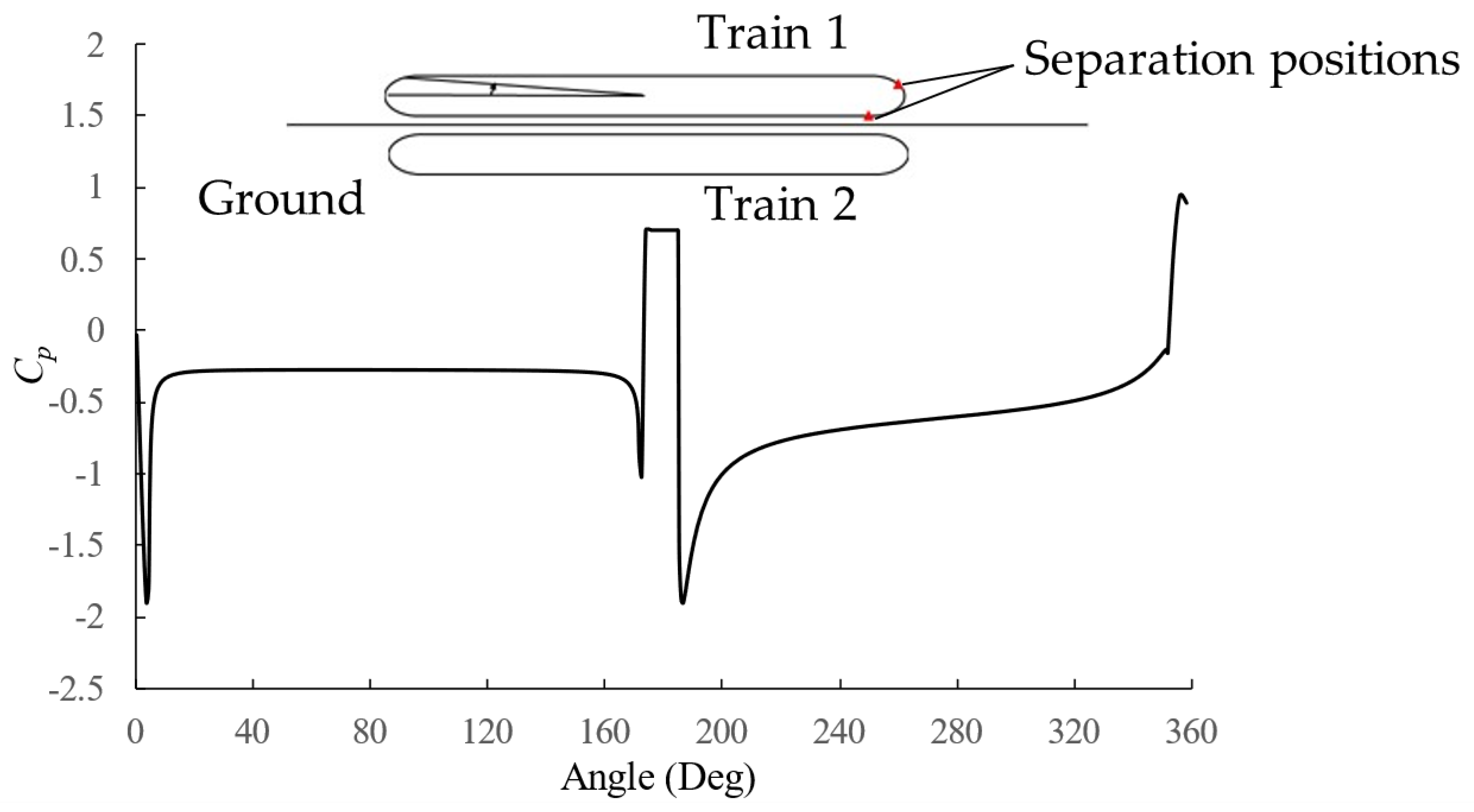
The influences of different nose shapes on the aerodynamic pressure loads of the train are investigated in this paper. The comparison of the nose lengths for Nose 1, Nose 2, and Nose 3 is presented in Figure 11, for which the values are 0.96 Dtr, 1.28 Dtr, and 1.6 Dtr, respectively. It can be concluded from Figure 11 that the peak values that appear just downstream of the stagnation position decrease with the increment of the nose length. The peak values just upstream do not have the same trend with the increase of the nose length, but the differences between the two peak values shrink as the nose length increases. One of the main features of the train is that it is running on the rails and is close to the ground while cruising. The presence of the ground must be considered when investigating the flow around the train. The method of images is employed in this case to model a solid ground at z = 0 by placing the mirror image of the 2-D train at the negative value of the height, which is 0.15 from the ground plane, as shown in Figure 12, where the number 1 refers to the 2-D train and the number 2 refers to the image. The method of images involves the analysis of the flow over multiple bodies, even if the original problem is for flow over a single solid body. In addition, as the solid bodies are symmetric at about z = 0 at the ground plane, the no-penetration condition is satisfied. A total of 200 panels were used in the simulation, including the ground effect. Unlike the symmetrical simulation above, the introduction of the ground plane leads to the flow around the train to be asymmetrical. According to the integral boundary-layer prediction, the separation positions with the presence of ground is not symmetric on the upper and lower surface of the train. They are about 176° on the upper surface and 186° on the lower surface in this case, as shown in Figure 12.
The asymmetry of the separation points leads to the difference in the wake panel lengths on the upper surface and the lower surface of the train. Thus, the interpolative procedure, as elaborated above, was conducted for the upper surface and the lower surface of the train, respectively. The determined “correct” lengths for the upper wake panel is 4 Dtr and for the lower wake panel is 9 Dtr.
For the asymmetric case, the pressure distribution on the upper and lower surface is different. The pressure distribution on the upper surface is similar to the symmetric case, but with a larger minimum pressure value in the head. On the lower surface, the pressure drops in the head and then remains almost constant until near the separation, where the pressure decreases slightly and then increases to meet the base pressure. Due to the asymmetry of the flow field, the stagnation moved slightly downward to the ground plane direction, which can be seen from the pressure distribution in Figure 12.
The effects of the ground clearance on the aerodynamic pressure loads of the train are also studied in the present work, as shown in Figure 13. Three different heights of the train are studied, which are h = 0.1, 0.15, and 0.2. It can be concluded from Figure 13 that that the ground clearance has little influence on the upper surface of the train. However, the pressure loads on the lower surface of the train increase with the decrease in the heights.

4. Conclusions

A 2-D separated-flow model based on the constant source/vortex panel method is proposed in this paper. The proposed model includes constant source panels to model the obstacle in the flow field and constant vortex panels to model the wake behind the body. To simulate the flow separation, the integral boundary-layer method is adapted to calculate the separation locations and an interpolative calculation is adapted to calculate the “correct” wake length for modelling the wake.
The proposed method is validated by comparing the calculated pressure distribution on a 2-D circular cylinder with the experimental data. The predicted separation location agrees well with the experiment, which proves the feasibility of incorporating the integral boundary-layer approximation in the separated-flow model. Additionally, the calculated pressure loads distributed on the train agree with the experimental results. This proves that the proposed model is credible in simulating flows around bluff bodies. Moreover, simulations with different panel densities are performed and the grid independency of the proposed method is verified by the results.
The proposed method is also applied to predict the pressure distribution along a 2-D generic train surface. According to the simulation results, the pressure changes dramatically at the front of the train. The flow then separates at the rear part of the train, with symmetrical separation locations in the absence of the ground configuration. The base pressure remains constant at the rear part of the train. Furthermore, the grid independency is validated in the 2-D train case by comparing the results of three different panel densities. In addition, the presence of the ground changes the pressure distribution pattern on the lower surface of the train: it weakens the pressure peak occurring around in the head and tail and increases the pressure on the underbody of the train. The stagnation position at the head of the train moves downward with the presence of the ground.
As the first stage to develop the numerical model for trains in tunnels, the presented method is capable of predicting the pressure distribution along arbitrary bluff bodies such as trains with flow separations. The most outstanding feature of the proposed method is that it saves tremendous computational time and resources comparing with high fidelity CFD simulations in pressure prediction. As a meshless method, it also saves the time and energy to construct a computational mesh. However, this method still needs improvements and modifications, for example, the effect of the compressibility, in order to be practised on other train aerodynamic applications such as the modelling of trains in tunnels.

Author Contributions

Conceptualization, H.H.; funding acquisition, J.X. and Y.J.; investigation, R.L.; supervision, H.H.; writing—original draft, R.L.; writing—review and editing, D.S. and J.N. All authors have read and agreed to the published version of the manuscript.

Funding

This research was funded by the National Natural Science Foundation of China, grant numbers 11962014 and 51965033.

Institutional Review Board Statement

Not applicable.

Informed Consent Statement

Not applicable.

Data Availability Statement

Not applicable.

Conflicts of Interest

The authors declare no conflict of interest.

References

  1. Buresti, G. Bluff-Body Aerodynamics; International Advanced School on Windexcited and Aeroelastic Vibrations of Structures: Genoa, Italy, 2000. [Google Scholar]
  2. Bearman, P. Bluff Body Flow Research with Application to Road Vehicles. In The Aerodynamics of Heavy Vehicles II: Trucks, Buses, and Trains; Lecture Notes in Applied and Computational Mechanics; Browand, F., McCallen, R., Ross, J., Eds.; Springer: Berlin, Heidelberg, 2009; Volume 41, pp. 3–13. [Google Scholar] [CrossRef]
  3. Flynn, D.; Hemida, H.; Soper, D.; Baker, C. Detached-eddy simulation of the slipstream of an operational freight train. J. Wind. Eng. Ind. Aerodyn. 2014, 132, 1–12. [Google Scholar] [CrossRef]
  4. Li, T.; Hemida, H.; Zhang, J.; Rashidi, M.; Flynn, D. Comparisons of Shear Stress Transport and Detached Eddy Simulations of the Flow Around Trains. J. Fluids. Eng. T ASME 2018, 140. [Google Scholar] [CrossRef]
  5. Morden, J.; Hemida, H.; Baker, C. Comparison of RANS and Detached Eddy Simulation Results to Wind-Tunnel Data for the Surface Pressures Upon a Class 43 High-Speed Train. J. Fluids Eng. 2015, 137. [Google Scholar] [CrossRef]
  6. Hemida, H.; Baker, C. Large-eddy simulation of the flow around a freight wagon subjected to a crosswind. Comput. Fluids 2010, 39, 1944–1956. [Google Scholar] [CrossRef]
  7. Hemida, H.; Krajnović, S. Exploring flow structures around a simplified ICE2 train subjected to a 30° side wind using LES. Eng. Appl. Comput. Fluid Mech. 2009, 3, 28–41. [Google Scholar] [CrossRef]
  8. Hemida, H.; Krajnović, S. LES study of the influence of the nose shape and yaw angles on flow structures around trains. J. Wind. Eng. Ind. Aerodyn. 2010, 98, 34–46. [Google Scholar] [CrossRef]
  9. Krajnović, S. Large eddy simulation of flows around ground vehicles and other bluff bodies. Philos. Trans. Royal Soc. A 2009, 367, 2917–2930. [Google Scholar] [CrossRef]
  10. Baker, C.; Johnson, T.; Flynn, D.; Hemida, H.; Quinn, A.; Soper, D.; Sterling, M. Train Aerodynamics, 1st ed.; Butterworth-Heinemann: Oxford, UK, 2019. [Google Scholar] [CrossRef]
  11. Jin, G.; Zou, L.; Jiang, Y.; Zong, Z.; Sun, Z. A circle theorem technique to handle 2-D flows around arbitrary cylinders in discrete vortex method. J. Wind. Eng. Ind. Aerodyn. 2021, 209, 104496. [Google Scholar] [CrossRef]
  12. Mukesh, R.; Lingadurai, K.; Selvakumar, U. Airfoil shape optimization using non-traditional optimization technique and its validation. J. King Saud Univ. Sci. 2014, 26, 191–197. [Google Scholar] [CrossRef]
  13. Rakhsha, M.; Kees, C.E.; Negrut, D. Lagrangian vs. Eulerian: An Analysis of Two Solution Methods for Free-Surface Flows and Fluid Solid Interaction Problems. Fluids 2021, 6, 460. [Google Scholar] [CrossRef]
  14. Moraes, P.G.; Alcântara Pereira, L.A. Surface Roughness Effects on Flows Past Two Circular Cylinders in Tandem Arrangement at Co-Shedding Regime. Energies 2021, 14, 8237. [Google Scholar] [CrossRef]
  15. Bellenoue, M.; Moriniere, V.; Kageyama, T. Experimental 3-D simulation of the compression wave, due to train–tunnel entry. J. Fluids Struct. 2002, 16, 581–595. [Google Scholar] [CrossRef]
  16. Yoon, T.S.; Lee, S.; Hwang, J.H.; Lee, D.H. Prediction and validation on the sonic boom by a high-speed train entering a tunnel. J. Sound Vib. 2001, 247, 195–211. [Google Scholar] [CrossRef]
  17. Rivero, J.M.; González-Martínez, E.; Rodríguez-Fernández, M. A methodology for the prediction of the sonic boom in tunnels of high-speed trains. J. Sound Vib. 2019, 446, 37–56. [Google Scholar] [CrossRef]
  18. Vardy, A.E.; Brown, J.M.B. Influence of ballast on wave steepening in tunnels. J. Sound Vib. 2000, 238, 595–615. [Google Scholar] [CrossRef]
  19. Ku, Y.C.; Rho, J.H.; Yun, S.H.; Kwak, M.H.; Kim, K.H.; Kwon, H.B.; Lee, D.H. Optimal cross-sectional area distribution of a high-speed train nose to minimize the tunnel micro-pressure wave. Struct. Multidisc. Optim. 2010, 42, 965–976. [Google Scholar] [CrossRef]
  20. Hess, J. Panel methods in computational fluid dynamics. Annu. Rev. Fluid Mech. 1990, 22, 255–274. [Google Scholar] [CrossRef]
  21. Baker, C. The flow around high speed trains. J. Wind. Eng. Ind. Aerodyn. 2010, 98, 277–298. [Google Scholar] [CrossRef]
  22. Baker, C. A review of train aerodynamics Part 1—Fundamentals. Aeronaut. J. 2014, 118, 201–228. [Google Scholar] [CrossRef]
  23. Hemida, H.; Baker, C.; Gao, G. The calculation of train slipstreams using large-eddy simulation. Proc. Inst. Mech. Eng. Pt. F J. Rail Rapid Transit. 2014, 228, 25–36. [Google Scholar] [CrossRef]
  24. Steinheuer, J. Aerodynamische Wirkungen Von Schnellfahrenden Schienenfahrzeugen Auf Die Umgebung; DFVLR-Bericht IB: Göttingen, Germany, 1981; pp. 129–181. [Google Scholar]
  25. Sanz-Andrés, A.; Santiago-Prowald, J.; Baker, C.; Quinn, A. Vehicle-induced loads on traffic sign panels. J. Wind. Eng. Ind. Aerodyn. 2003, 91, 925–942. [Google Scholar] [CrossRef]
  26. Sanz-Andrés, A.; Laverón, A.; Cuerva, A.; Baker, C. Vehicle-induced force on pedestrians. J. Wind. Eng. Ind. Aerodyn. 2004, 92, 185–198. [Google Scholar] [CrossRef]
  27. Sanz-Andrés, A.; Laverón, A.; Baker, C.; Quinn, A. Vehicle induced loads on pedestrian barriers. J. Wind. Eng. Ind. Aerodyn. 2004, 92, 413–426. [Google Scholar] [CrossRef]
  28. Sanz-Andrés, A.; Santiago-Prowald, J. Train-induced pressure on pedestrians. J. Wind. Eng. Ind. Aerodyn. 2002, 90, 1007–1015. [Google Scholar] [CrossRef]
  29. Barrero-Gil, A.; Sanz-Andrés, A. Aeroelastic effects in a traffic sign panel induced by a passing vehicle. J. Wind. Eng. Ind. Aerodyn. 2009, 97, 298–303. [Google Scholar] [CrossRef]
  30. Rutschmann, S.; Ehenfried, K.; Dillmann, A. Validation of a potential flow model for the prediction of the aerodynamic loads on track side objects. In Proceedings of the World Congress on Rail Research, Sydney, Australia, 25–28 November 2013. [Google Scholar]
  31. Rutschmann, S.; Ehrenfried, K.; Dillmann, A. Aerodynamic loads induced by passing trains on track side objects. Notes Numer. Fluid Mech. Multidiscip. Des. 2014, 124, 343–351. [Google Scholar] [CrossRef]
  32. Katz, J.; Plotkin, A. Low-Speed Aerodynamics; Cambridge University Press: Cambridge, UK, 2001. [Google Scholar] [CrossRef]
  33. Hermanns, L.; Giménez, J.; Alarcón, E. Efficient computation of the pressures developed during high-speed train passing events. Comput. Struct. 2005, 83, 793–803. [Google Scholar] [CrossRef] [Green Version]
  34. Takei, Y.; Izumi, Y.; Yamada, S.; Iida, M.; Kikuchi, K. Evaluation method for air pressure variation and station facility member deterioration caused by high-speed train passage in stations. Q. Rep. RTRI 2008, 49, 89–95. [Google Scholar] [CrossRef]
  35. Kikuchi, K.; Uchida, K.; Nakatani, K.; Yoshida, Y.; Maeda, T.; Yanagizawa, M. Numerical Analysis of Pressure Variation due to Train Passage Using the Boundary Element Method. Q. Rep. RTRI 1996, 37, 231–237. [Google Scholar]
  36. Khandhia, Y.; Gaylard, A.; Johnson, T. CFD simulation of three-dimensional unsteady train aerodynamics. Veh. Aerodyn. 1996, 10, 82–93. [Google Scholar]
  37. Johnston, G.; Seshagiri, B.; Ellis, N. Aerodynamic Interference of High Speed Ground Vehicles. In UTIAS Report, No. 185; University of Toronto: Toronto, ON, Canada, 1976; Available online: https://repository.tudelft.nl/islandora/object/uuid%3Acc2955c7-7f39-4c43-951c-8becc39c1530 (accessed on 11 September 2022).
  38. Morrow, T. Prediction of the Pressure Distribution on Vehicles Moving Near the Ground; Report No. TT72R05; Department of Transport Technology, Loughborough University of Technology: Loughborough, UK, 1972. [Google Scholar]
  39. Reinhardt-Piéchowiak, A.; Ducruet, C. Inviscid fluid flow around high-speed trains passing by in open air. Proc. Inst. Mech. Eng. Pt. F J. Rail Rapid Transit. 1999, 213, 105–116. [Google Scholar] [CrossRef]
  40. Bérenger, T.; Grégoire, R. Part 2: Panel Method Applied to Problems of European High-speed Train Interoperability. In TRANSAERO—A European Initiative on Transient Aerodynamics for Railway System Optimisation. Notes on Numerical Fluid Mechanics and Multidisciplinary Design (NNFM); Schulte-Werning, B., Grégoire, R., Malfatti, A., Matschke, G., Eds.; Springer: Berlin/Heidelberg, Germany, 2002; Volume 79. [Google Scholar] [CrossRef]
  41. Bérenger, T.; Kessler, A.; Grégoire, R. Part 1: Panel Method Applied to the Prediction of Unsteady Effects Caused by High-speed Trains Passing in the Open Air. In TRANSAERO—A European Initiative on Transient Aerodynamics for Railway System Optimisation. Notes on Numerical Fluid Mechanics and Multidisciplinary Design (NNFM); Schulte-Werning, B., Grégoire, R., Malfatti, A., Matschke, G., Eds.; Springer: Berlin/Heidelberg, Germany, 2002; Volume 79. [Google Scholar] [CrossRef]
  42. Farhan, I. Theoretical and Experimental Aerodynamic Analysis for High-Speed Ground Vehicles. Ph.D. Thesis, Department of Aeronautical and Automotive Engineering, Loughborough University, Loughborough, UK, 1991. Available online: https://hdl.handle.net/2134/22236 (accessed on 11 September 2022).
  43. Mahomedali, F. Two-dimensional potential flow calculations applied to train cross-section. In Internal Memorandum, IM AERO 67; British Railways Board, Research and Development Division, Aerodynamics Section: London, UK, 1973. [Google Scholar]
  44. Copley, J. The Three-Dimensional Flow around Railway Trains. Ph.D. Thesis, Department of Engineering, University of Cambridge, Cambridge, UK, 1985. [Google Scholar]
  45. Copley, J. The Three-Dimensional Flow around Railway Trains. J. Wind. Eng. Ind. Aerodyn. 1987, 26, 21–52. [Google Scholar] [CrossRef]
  46. Chiu, T. Aerodynamic Loads on a Railway Train in a Cross-Wind at Large Yaw Angles. Ph.D. Thesis, Churchill College, University of Cambridge, Cambridge, UK, 1990. [Google Scholar]
  47. Chiu, T. A two-dimensional second-order vortex panel method for the flow in a cross-wind over a train and other two-dimensional bluff bodies. J. Wind. Eng. Ind. Aerodyn. 1991, 37, 43–64. [Google Scholar] [CrossRef]
  48. Chiu, T. Prediction of the aerodynamic loads on a railway train in a cross-wind at large yaw angles using an integrated two- and three-dimensional source/vortex panel method. J. Wind. Eng. Ind. Aerodyn. 1995, 57, 19–39. [Google Scholar] [CrossRef]
  49. Tyll, J. Concurrent Aerodynamic Shape/Cost Design of Magnetic Levitation Vehicles Using Multidisciplinary Design Optimization Techniques. Ph.D. Thesis, Aerospace Engineering, Virginia Polytechnic Institute and State University, Blacksburg, VA, USA, 1997. [Google Scholar]
  50. Dvorak, F.; Maskew, B.; Woodward, F. Investigation of Three-Dimensional Flow Separation on Fuselage Configurations; US Army AMRDL Report TR-77-4; Analytical Methods Inc.: Bellevue, WA, USA, 1997. [Google Scholar]
  51. Balleur, J. Strong matching method for computing transonic viscous flows including wakes and separations. La Recherche Aérospatiale 1981, 3, 21–45. [Google Scholar]
  52. Drela, M.; Giles, M. Viscous-inviscid analysis of transonic and low Reynolds number airfoils. AIAA J. 1987, 25, 1347–1355. [Google Scholar] [CrossRef]
  53. White, F. Viscous Fluid Flow, 3rd ed.; McGraw-Hill: New York, NY, USA, 2006. [Google Scholar]
  54. Thwaites, B. Approximate Calculation of the Laminar Boundary Layer. Aeronaut. Q. 1949, 1, 245–280. [Google Scholar] [CrossRef]
  55. Whitfield, D.; Swafford, T.; Jacocks, J. Calculation of turbulent boundary layers with separation and viscous-inviscid interaction. AIAA J. 1981, 19, 1315–1322. [Google Scholar] [CrossRef]
  56. Smith, A. Transition, Pressure Gradient and Stability Theory; Report ES 26388; Douglas Aircraft Co.: Santa Monica, CA, USA, 1956; Available online: https://ci.nii.ac.jp/naid/10008210731 (accessed on 11 September 2022).
  57. Van Ingen, J. A suggested semi-empirical method for the calculation of the boundary layer transition region. In Technische Hogeschool Delft, Vliegtuigbouwkunde, Rapport VTH-74; Delft University of Technology: Delft, The Netherlands, 1956. [Google Scholar]
  58. Green, J.; Weeks, D.; Brooman, J. Prediction of Turbulent Boundary Layers and Wakes in Compressible Flow by a Lag-Entrainment Method; R&M Report 3643; Aeronautical Research Council, HMSO: London, UK, 1973; Available online: https://apps.dtic.mil/sti/citations/ADA041015 (accessed on 11 September 2022).
  59. Head, M.; Patel, V. Improved Entrainment Turbulent Boundary Method for Calculating Layer Development; R&M Report 3791; Aeronautical Research Council, HMSO: London, UK, 1968; Available online: https://reports.aerade.cranfield.ac.uk/handle/1826.2/2913 (accessed on 11 September 2022).
  60. Drela, M. Aerodynamics of Viscous Flows (Draft); Massachusetts Institute of Technology: Cambridge, MA, USA, 2016. [Google Scholar]
  61. Roshko, A. Experiments on the flow past a circular cylinder at very high Reynolds number. J. Fluid Mech. 1961, 10, 345–356. [Google Scholar] [CrossRef]
  62. Chiu, T.; Squire, L. An experimental study of the flow over a train in a crosswind at large yaw angles up to 90°. J. Wind. Eng. Ind. Aerodyn. 1992, 45, 47–74. [Google Scholar] [CrossRef]
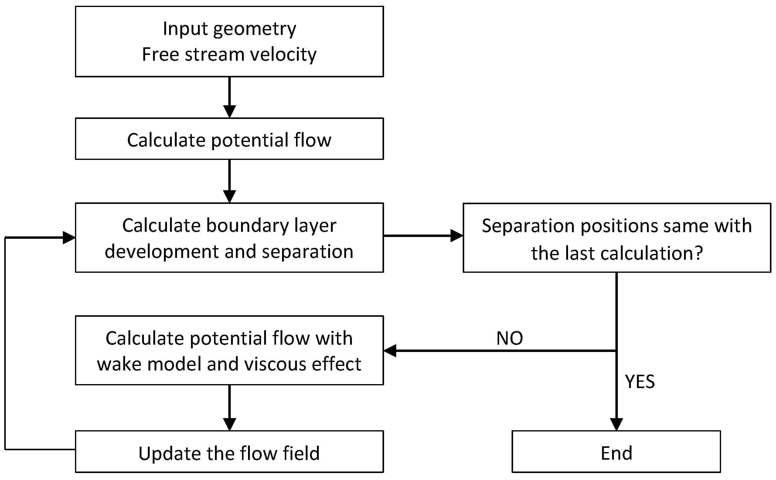
Figure 1. Flow diagram of the calculation procedure.
Applsci 12 09652 g001
Figure 2. Sketch of boundary discretisation and separated-flow model.
Applsci 12 09652 g002
Figure 3. Calculation of tangential velocity increment along the wake panel.
Applsci 12 09652 g003
Figure 4. Simulation results for a circular cylinder at Re = 1 × 10⁷: (a) flow field around the circular cylinder; (b) pressure distribution on half of the cylinder.
Applsci 12 09652 g004
Figure 5. Distributions of tangential velocity increment on a circular cylinder for various wake lengths.
Applsci 12 09652 g005
Figure 6. Results from the iterative wake length procedure applied to a circular cylinder.
Applsci 12 09652 g006
Figure 7. Generic train model.
Applsci 12 09652 g007
Figure 8. Distributions of tangential velocity increment on the train for various wake lengths.
Applsci 12 09652 g008
Figure 9. Pressure distribution on the train with different panel densities without the ground.
Applsci 12 09652 g009
Figure 10. Results from the iterative wake length procedure of the train.
Applsci 12 09652 g010
Figure 11. Comparison of the pressure distributions on trains with different nose shapes.
Applsci 12 09652 g011
Figure 12. Pressure distribution on the train with the ground configuration.
Applsci 12 09652 g012
Figure 13. Comparison of pressure distributions on the trains with different ground clearance.
Applsci 12 09652 g013
Table 1. Comparison of peak values and base pressure for trains with different panel numbers.
Position100 Panels200 Panels300 Panels
CpPositionCpPositionCpPosition
1−1.124.6°−1.195.2°−1.215.4°
2−0.41171.8°−0.7173.0°−0.6173.4°
3−0.41185°−0.7185.5°−0.6185.8°
4−1.12352.6°−1.19353.5°−1.21353.9°
Base pressure−0.34−0.3−0.36
Publisher’s Note: MDPI stays neutral with regard to jurisdictional claims in published maps and institutional affiliations.