
Numerical Investigation of the Influence of the Wake of Wind Turbines with Different Scales Based on OpenFOAM


Abstract
:1. Introduction
2. Project Overview
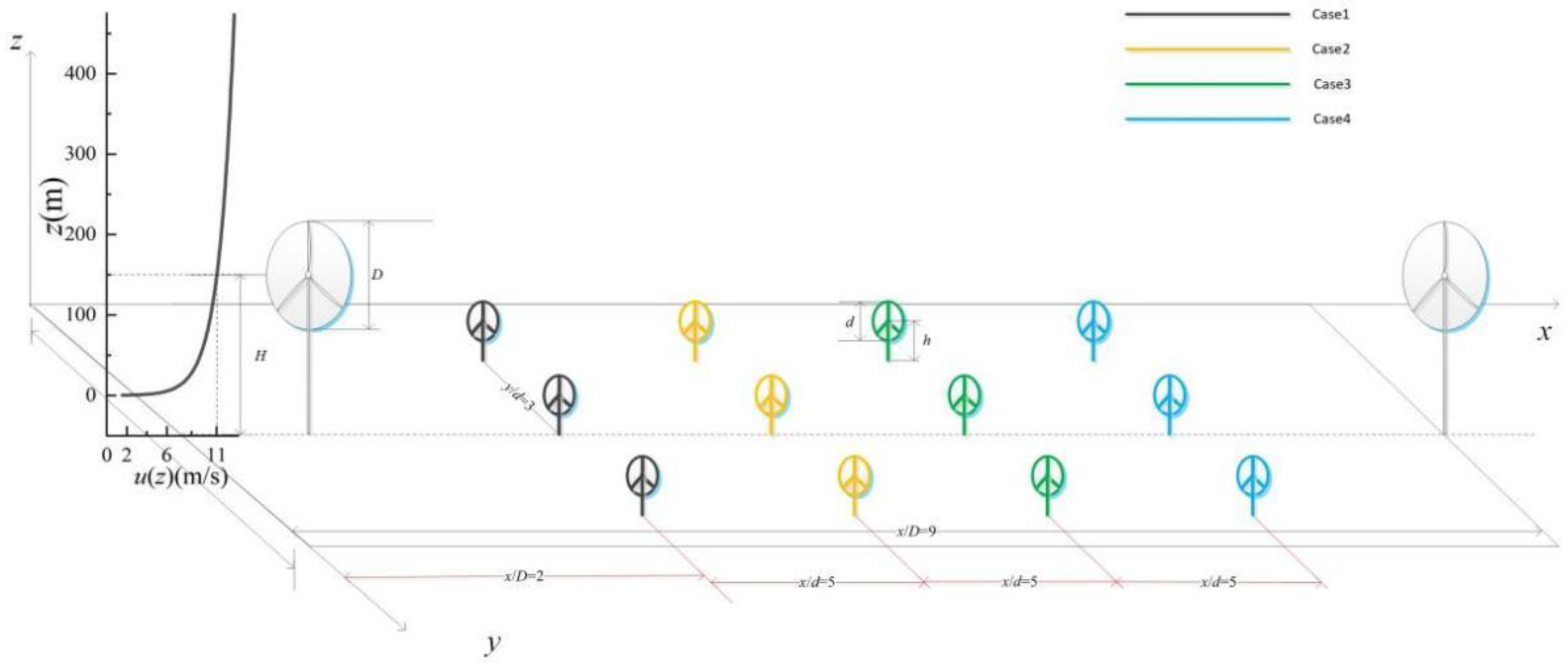
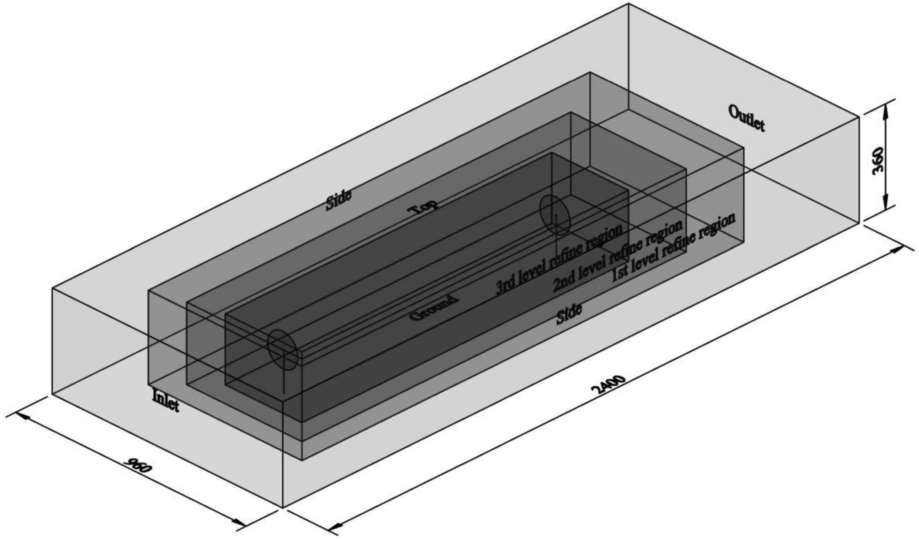
2.1. Simulation
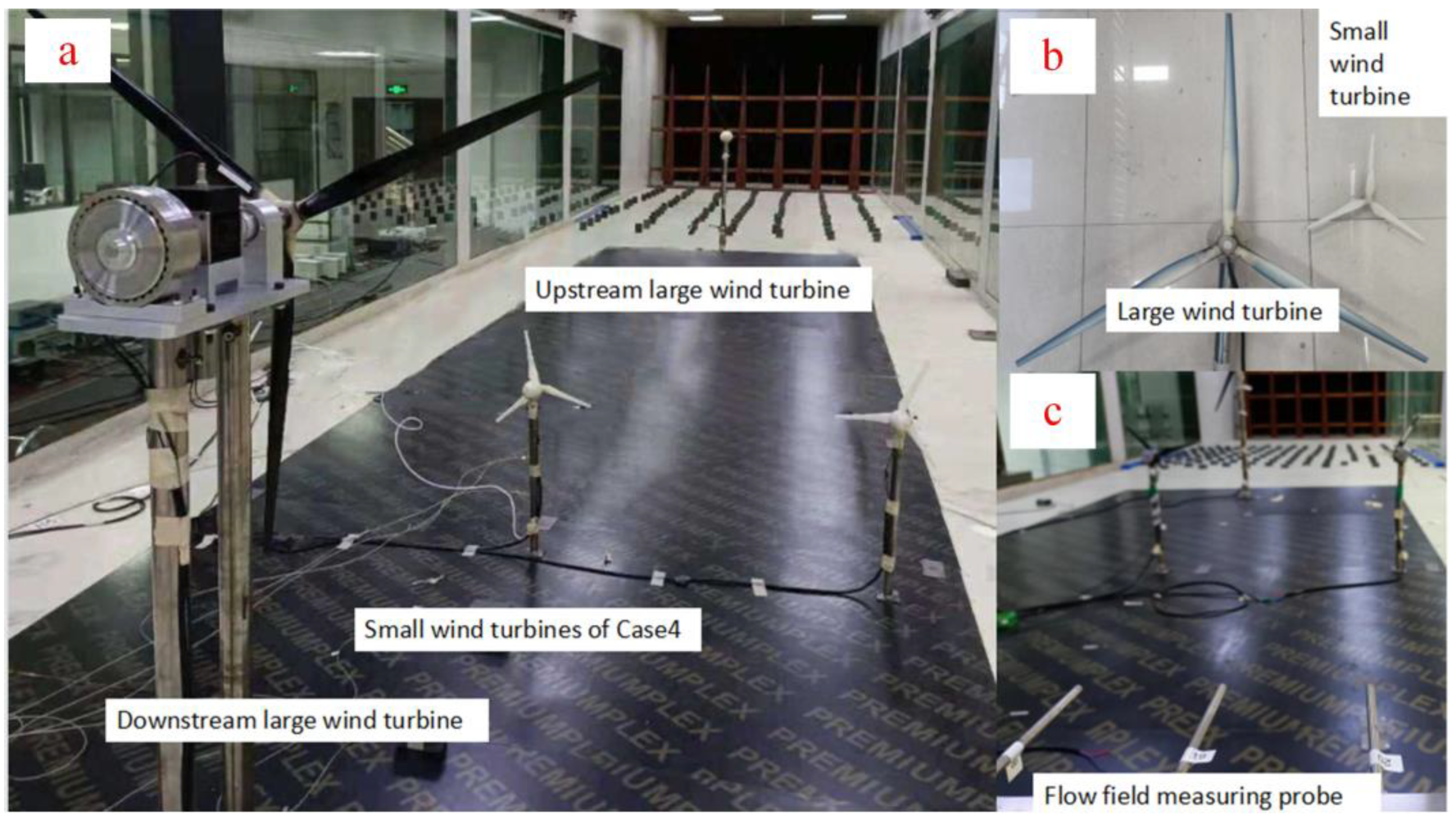
2.2. Wind Tunnel Test
3. Results and Discussions
3.1. Power of Large Wind Turbines
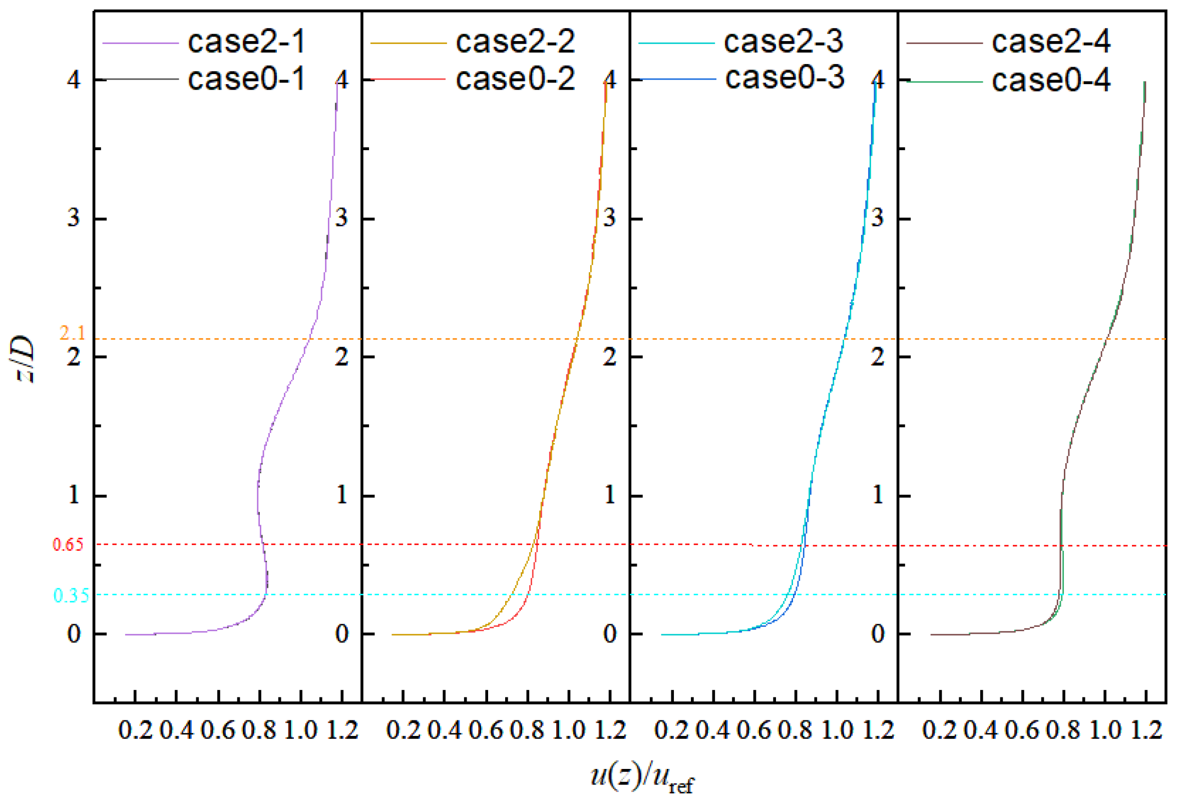
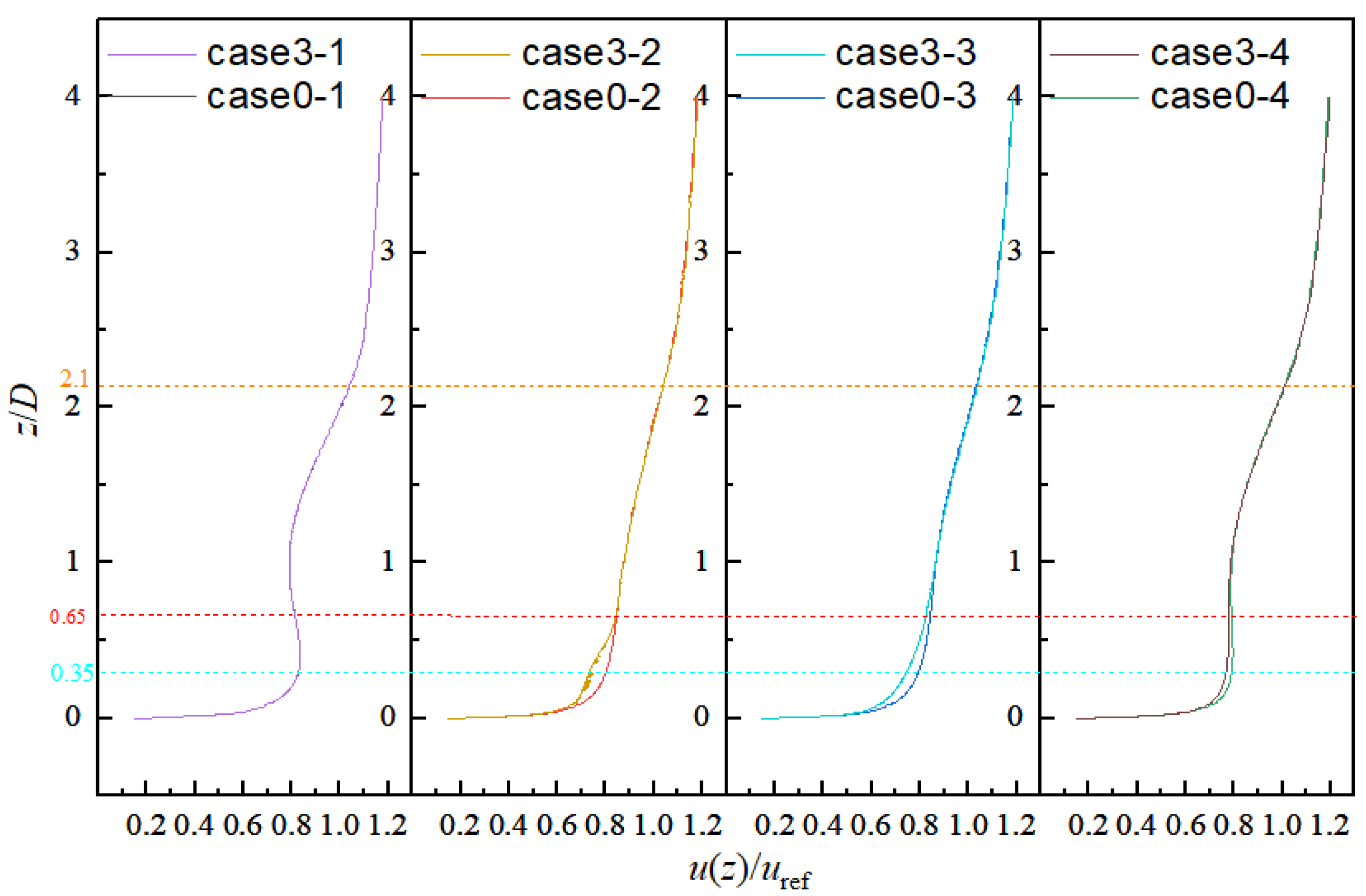
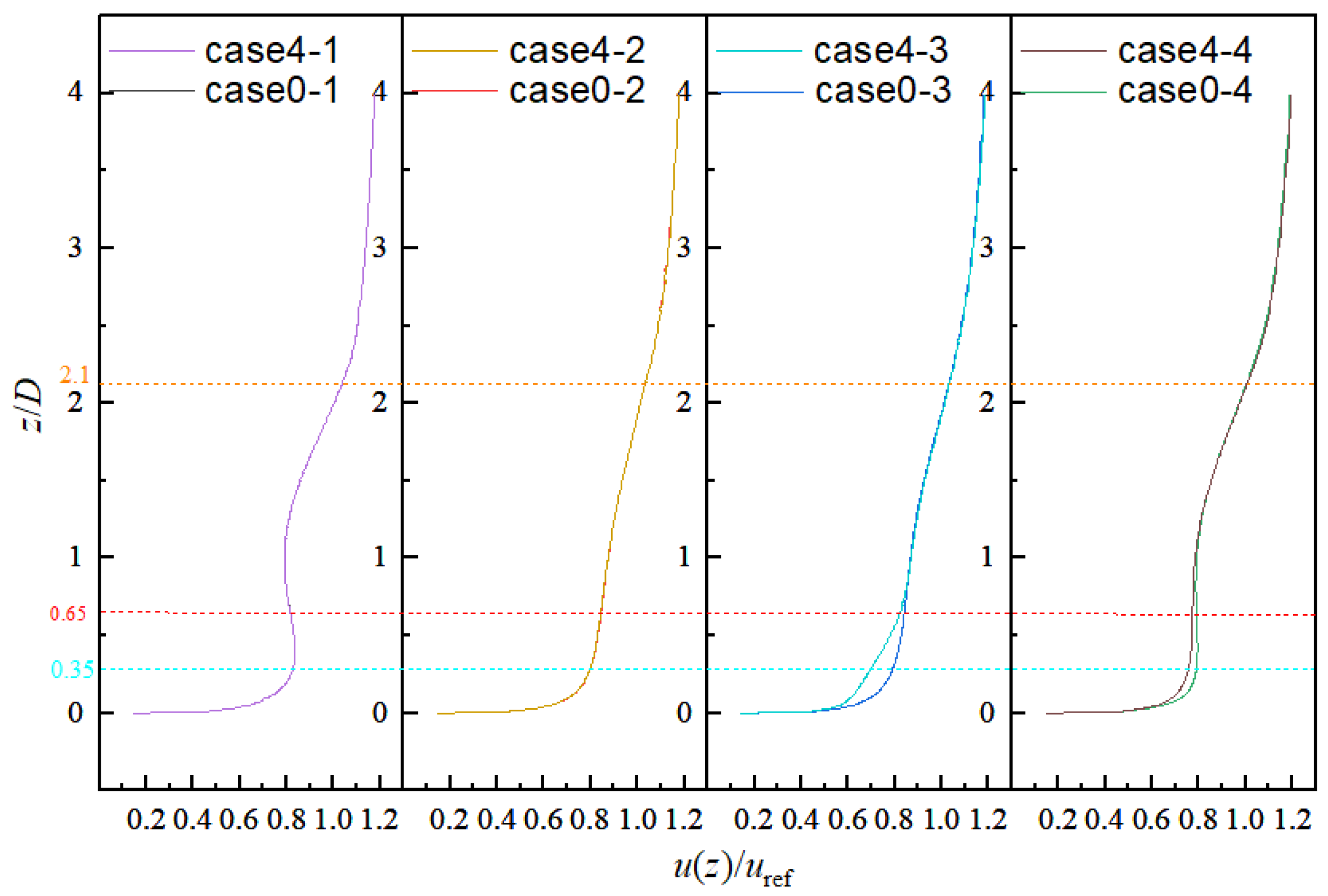
3.2. Vertical Velocity Distribution in the Flow Field
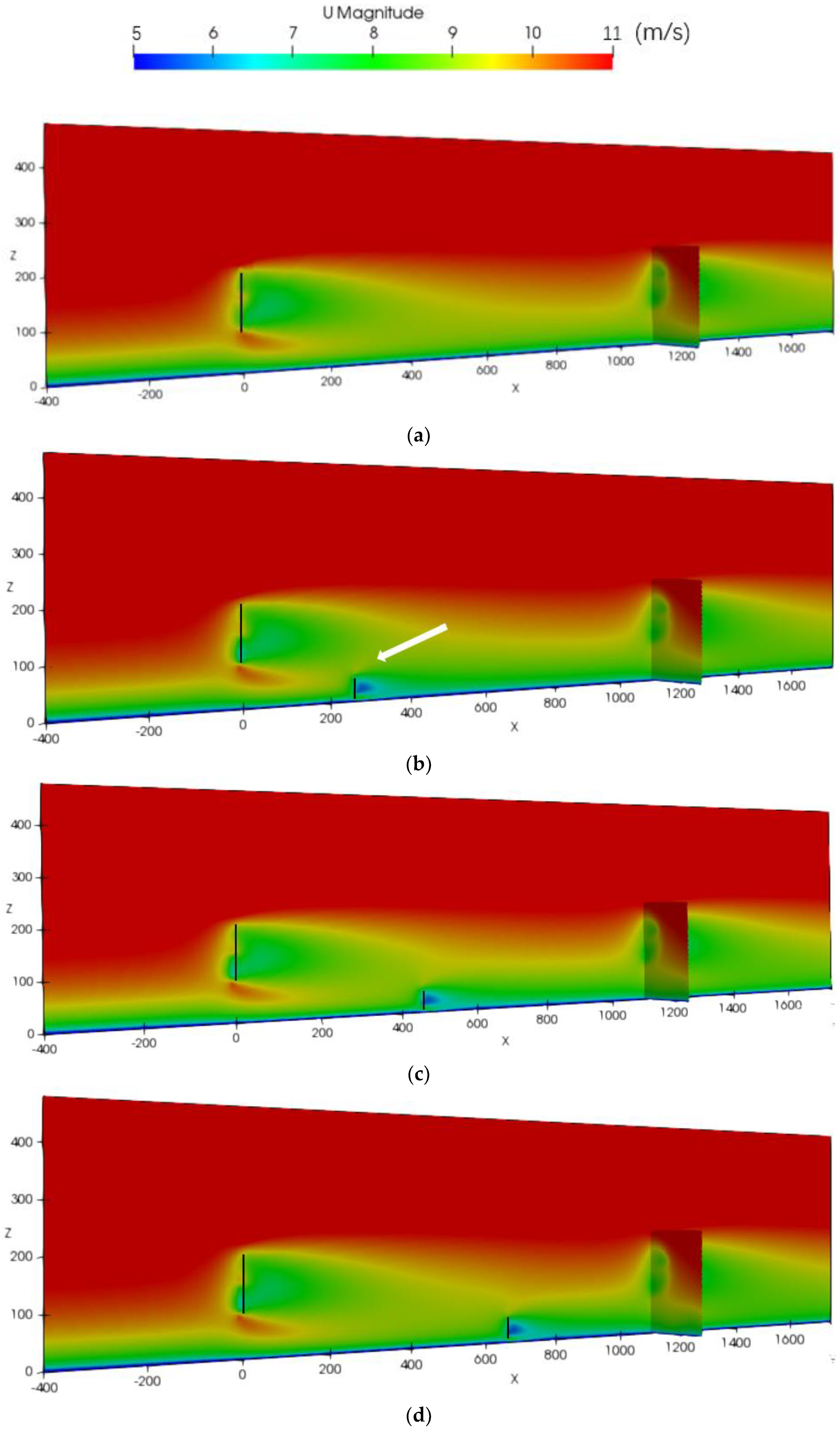
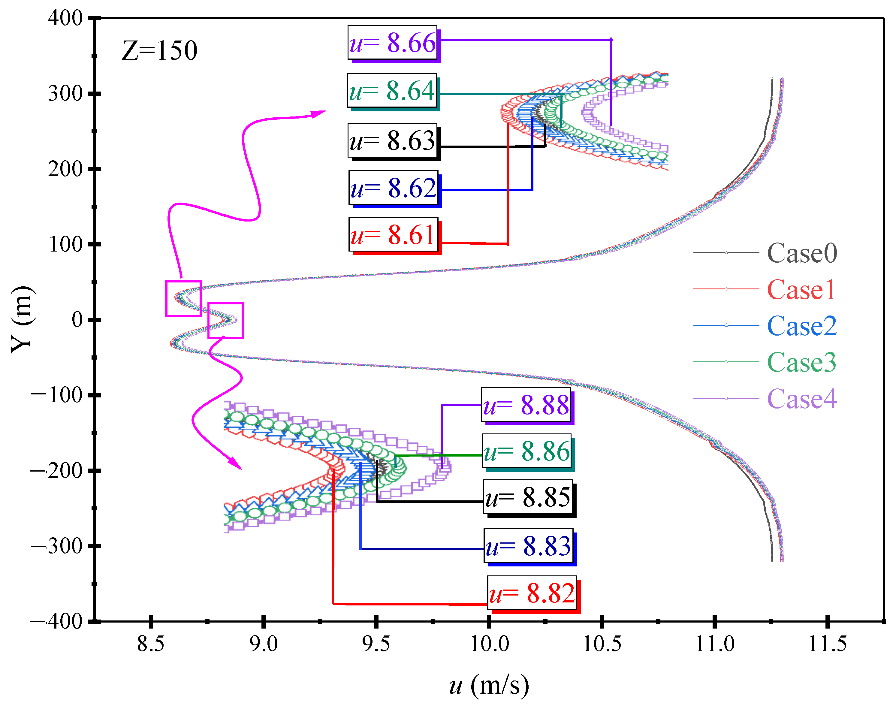
3.3. Velocity Field Distribution under Different Operating Conditions
4. Conclusions
- (1)
- Small wind turbines with different distances have an impact on the power output of downstream wind turbines. The power of the downstream large wind turbine increases by about 0.5% when the small and large wind turbines are 2D + 15d away from the upstream large wind turbines, as in Case 4. The wind tunnel experiment results also show that the power of the downstream large wind turbine increases by 0.69%.
- (2)
- At the height of the small wind turbine, the velocity distribution of the wake obviously attenuates, and this attenuation will weaken as it moves downstream; however, the wind speed at the higher position of the small wind turbine will increase, and this increase effect will be captured by the adjacent downstream large wind turbine, resulting in an increase in the output power of the downstream large wind turbine.
Author Contributions
Funding
Institutional Review Board Statement
Informed Consent Statement
Data Availability Statement
Conflicts of Interest
References
- Zhang, L.D.; Li, Y.; Zhang, H.; Xu, X.D. A review of the potential of district heating system in Northern China. Appl. Therm. Eng. 2021, 188, 116605. [Google Scholar] [CrossRef]
- Zhao, Z.Z.; Jiang, R.F.; Feng, J.X.; Liu, H.W. Researches on vortex generators applied to wind turbines: A review. Ocean Eng. 2022, 253, 111266. [Google Scholar] [CrossRef]
- Zhao, X.Y.; Hu, T.Y.; Zhang, L.D.; Yang, Z.L. Experimental study on the characteristics of wind turbine wake field considering yaw conditions. Energy Sci. Eng. 2021, 9, 2333–2341. [Google Scholar] [CrossRef]
- Ali, C.K.; Ryozo, N. A quantitative review of wind farm control with the objective of wind farm power maximization. J. Wind Eng. Ind. Aerodyn. 2019, 192, 45–73. [Google Scholar]
- Stanley, A.; Ning, A.; Dykes, K. Optimization of turbine design in wind farms with multiple hub heights, using exact analytic gradients and structural constraints. Wind Energy 2019, 22, 605–619. [Google Scholar] [CrossRef]
- Mao, Y.; Shi, C.Y.; Liu, H.Y. Day-ahead wind power forecasting based on the clustering of equivalent power curves. Energy 2021, 218, 119515. [Google Scholar]
- Li, X.Y.; Qiu, Y.N.; Feng, Y.H.; Wang, Z. Wind turbine power prediction considering wake effects with dual laser beam LiDAR measured yaw misalignment. Appl. Energy 2021, 299, 117308. [Google Scholar] [CrossRef]
- Chen, Y.; Li, H.; Jin, K.; Elkassabgi, K. Investigating the possibility of using different hub height wind turbines in a wind farm. Int. J. Sustain. Energy 2017, 36, 142–150. [Google Scholar] [CrossRef]
- Vasel-Be-Hagh, A.; Archer, C.L. Wind farm hub height optimization. Appl. Energy 2017, 195, 905–921. [Google Scholar] [CrossRef]
- Wang, L.Y. Effectiveness of optimized control strategy and different hub height turbines on a real wind farm optimization. Renew. Energy 2018, 126, 819–829. [Google Scholar] [CrossRef]
- Mo, J.; Choudhry, A.; Arjomandi, M.; Lee, Y. Large eddy simulation of the wind turbine wake characteristics in the numerical wind tunnel model. J. Wind Eng. Ind. Aerodyn. 2013, 112, 11–24. [Google Scholar] [CrossRef]
- Sanne, J.H.; Magnus, K.V.; Antonio, S.; Nicholas, A. A comparison of lab-scale free rotating wind turbines and actuator disks. J. Wind Eng. Ind. Aerodyn. 2021, 209, 104485. [Google Scholar]
- Bontempo, R.; Manna, M. A ring-vortex actuator disk method for wind turbines including hub effects. Energy Convers. Manag. 2019, 195, 672–681. [Google Scholar] [CrossRef]
- Abdolrahim, R.; Micallef, D. Wake interactions of two tandem floating offshore wind turbines: CFD analysis using actuator disc model. Renew. Energy 2021, 179, 859–876. [Google Scholar]
- Daniel, M.; Carlos, F.; Iván, H.; Leo, H. Assessment of actuator disc models in predicting radial flow and wake expansion. J. Wind Eng. Ind. Aerodyn. 2020, 207, 104396. [Google Scholar]
- Ingrid, N.; Michael, H.; Jonathan, W.; Joachim, P. Comparison of the turbulence in the wakes of an actuator disc and a model wind turbine by higher order statistics: A wind tunnel study. Renew. Energy 2021, 179, 1650–1662. [Google Scholar]
- Hamlaoui, M.N.; Smaili, A.; Dobrev, I.; Pereira, M. Numerical and experimental investigations of HAWT near wake predictions using Particle Image Velocimetry and Actuator Disk Method. Energy 2022, 238, 121660. [Google Scholar] [CrossRef]
- Mehtab, A.K.; Adeel, J.; Sehar, S.; Abdul, H.S. Optimization of a wind farm by coupled actuator disk and mesoscale models to mitigate neighboring wind farm wake interference from repowering perspective. Appl. Energy 2021, 298, 117229. [Google Scholar]
- Yu, W.; Ferreira, C.; Kuik, G.A.M. The dynamic wake of an actuator disc undergoing transient load: A numerical and experimental study. Renew. Energy 2019, 132, 1402–1414. [Google Scholar] [CrossRef]
- Stevens, R.J.A.M.; Martínez-Tossas, L.; Meneveau, C. Comparison of wind farm large eddy simulations using actuator disk and actuator line models with wind tunnel experiments. Renew. Energy 2018, 116, 470–478. [Google Scholar] [CrossRef]
- Jiang, R.; Zhao, Z.; Liu, H.; Wang, T.; Chen, M.; Feng, J.; Wang, D. Numerical study on the influence of vortex generators on wind turbine aerodynamic performance considering rotational effect. Renew. Energy 2022, 186, 730–741. [Google Scholar] [CrossRef]
- Chamorro, L.P.; Sotiropoulos, F. Turbulent flow inside and above a wind farm: A wind-tunnel study. Energies 2011, 4, 1916–1936. [Google Scholar] [CrossRef]
- Wu, Y.T.; Fernando, P. Modeling turbine wakes and power losses within a wind farm using LES: An application to the Horns Rev offshore wind farm. Renew. Energy 2015, 75, 945–955. [Google Scholar] [CrossRef]
- Lee, H.; Lee, D. Wake impact on aerodynamic characteristics of horizontal axis wind turbine under yawed flow conditions. Renew. Energy 2019, 136, 383–392. [Google Scholar] [CrossRef]
- Mereu, R.; Federici, D.; Ferrari, G.; Schito, P. Parametric numerical study of Savonius wind turbine interaction in a linear array. Renew. Energy 2017, 113, 1320–1332. [Google Scholar] [CrossRef]
- Rajagopal, V.B.; Santanu, M.; Pankaj, K. An OpenFOAM based study of Savonius turbine arrays in tunnels for power maximisation. Renew. Energy 2021, 179, 1345–1359. [Google Scholar]
- Shayesteh, A.; Mahmood, R.; Esmail, M.; Andres, J. Mohammad Hossein Abbaspour-Fard, Numerical simulation of the Mexico wind turbine using the actuator disk model along with the 3D correction of aerodynamic coefficients in OpenFOAM. Renew. Energy 2021, 163, 2029–2036. [Google Scholar]
- Churchfield, M.; Lee, S. NWTC Design Codes. Available online: http://wind.nrel.gov/designcodes/simulators/SOWFA (accessed on 5 September 2022).
- OpenFOAM. The Open Source CFD Toolbox. 2013. Available online: http://www.openfoam.com (accessed on 20 August 2022).
- Yang, Y.; Gu, M.; Chen, S.; Jin, X. New inflow boundary conditions for modelling the neutral equilibrium atmospheric boundary layer in computational wind engineering. J. Wind Eng. Ind. Aerodyn. 2009, 97, 88–95. [Google Scholar] [CrossRef]
- Hargreaves, D.M.; Wright, N.G. On the use of the k–ε model in commercial CFD software to model the neutral atmospheric boundary layer. J. Wind Eng. Ind. Aerodyn. 2007, 95, 355–369. [Google Scholar] [CrossRef]
- Li, Y.; Tong, G.; Zhao, B.; Feng, F.; Tagawa, K. Study on aerodynamic performance of a straight-bladed VAWT using a wind-gathering device with polyline hexagonal pyramid shape. Front. Energy Res. 2022, 10, 790777. [Google Scholar] [CrossRef]
- Liu, L.; Stevens, R.J.A.M. Enhanced wind-farm performance using windbreaks. Phys. Rev. Fluids 2021, 6, 074611. [Google Scholar] [CrossRef]


| Parameters | Values |
|---|---|
| Domain, x × y × z (m) | 2400 × 960 × 320 |
| Diameters of large turbine D (m) | 126 |
| Hub height of large turbine H (m) | 150 |
| Diameters of small turbine d (m) | 42 |
| Hub height of small turbine h (m) | 37 |
| vref (m/s) | 11.2 |
| Case 0 | No small wind turbine |
| Case 1 | 2D |
| Case 2 | 2D + 5d |
| Case 3 | 2D + 10d |
| Case 4 | 2D + 15d |
| Patch Names | Flow Variable Fields | ||||
|---|---|---|---|---|---|
| u | p | k | ε | μt | |
| inlet | atmBoundaryLayerInletVelocity | zeroGradient | atmBoundaryLayerInletK | atmBoundaryLayerInletEpsilon | calculated |
| outlet | inletOutlet | fixedValue | inletOutlet | inletOutlet | calculated |
| side | symmetry | symmetry | symmetry | symmetry | symmetry |
| top | fixedShearStress | zeroGradient | zeroGradient | zeroGradient | calculated |
| ground | fixedValue | zeroGradient | kqRWallFunction | epsilonWallFunction | atmNutkWallFunction |
| Case No. | Grid Number of the Background Mesh | Cubic Cell-Size Adjacent to Wind Turbine Blades | Averaged y+ of the Ground Patch | Time-Averaged Power Output of the NREL 5-MW Turbines | |||
|---|---|---|---|---|---|---|---|
| Streamwise | Cross-Streamwise | Elevational | Upstream One | Downstream One | |||
| 1 | 200 | 80 | 266 | 1.5 m | 101 | 4,857,263 | 4,228,941 |
| 2 | 150 | 60 | 200 | 2.0 m | 145 | 4,839,404 | 4,218,299 |
| 3 | 120 | 48 | 160 | 2.5 m | 188 | 4,795,899 | 4,183,746 |
| 4 | 100 | 40 | 133 | 3.0 m | 235 | 4,724,876 | 4,128,258 |
| Parameters | Values |
|---|---|
| Diameters of large turbine De (mm) | 1000 |
| Hub height of large turbine He (mm) | 1200 |
| Diameters of small turbine de (mm) | 340 |
| Hub height of small turbine he (mm) | 300 |
| Inflow 11.2 m/s | Case 0 | Case 1 | Case 2 | Case 3 | Case 4 |
|---|---|---|---|---|---|
| Power of upstream large wind turbine | 4839.40 | 4833.47 | 4837.80 | 4839.02 | 4839.31 |
| Power of downstream large wind turbine | 4218.30 | 4194.38 | 4202.52 | 4215.43 | 4239.35 |
| Total power of the larger wind turbines | 9057.70 | 9027.85 | 9040.32 | 9054.45 | 9078.66 |
| Total power of the smaller wind turbines | 0 | 604.36 | 603.24 | 602.52 | 601.46 |
| Total power of the larger turbines and small wind turbines | 9057.70 | 9632.21 | 9643.56 | 9656.97 | 9680.12 |
| Inflow 7 m/s | Case 0 | Case 1 | Case 2 | Case 3 | Case 4 |
|---|---|---|---|---|---|
| Power of downstream wind turbine | 7028.1 | 6910.3 | 6996.2 | 6961.1 | 7076.5 |
| Increase | / | −1.67% | −0.45% | −0.96% | 0.69% |
Publisher’s Note: MDPI stays neutral with regard to jurisdictional claims in published maps and institutional affiliations. |
© 2022 by the authors. Licensee MDPI, Basel, Switzerland. This article is an open access article distributed under the terms and conditions of the Creative Commons Attribution (CC BY) license (https://creativecommons.org/licenses/by/4.0/).
Share and Cite
Tian, W.; Tie, H.; Ke, S.; Wan, J.; Zhao, X.; Zhao, Y.; Zhang, L.; Wang, S. Numerical Investigation of the Influence of the Wake of Wind Turbines with Different Scales Based on OpenFOAM. Appl. Sci. 2022, 12, 9624. https://doi.org/10.3390/app12199624
Tian W, Tie H, Ke S, Wan J, Zhao X, Zhao Y, Zhang L, Wang S. Numerical Investigation of the Influence of the Wake of Wind Turbines with Different Scales Based on OpenFOAM. Applied Sciences. 2022; 12(19):9624. https://doi.org/10.3390/app12199624
Chicago/Turabian StyleTian, Wenxin, Hao Tie, Shitang Ke, Jiawei Wan, Xiuyong Zhao, Yuze Zhao, Lidong Zhang, and Sheng Wang. 2022. "Numerical Investigation of the Influence of the Wake of Wind Turbines with Different Scales Based on OpenFOAM" Applied Sciences 12, no. 19: 9624. https://doi.org/10.3390/app12199624
APA StyleTian, W., Tie, H., Ke, S., Wan, J., Zhao, X., Zhao, Y., Zhang, L., & Wang, S. (2022). Numerical Investigation of the Influence of the Wake of Wind Turbines with Different Scales Based on OpenFOAM. Applied Sciences, 12(19), 9624. https://doi.org/10.3390/app12199624