Workforce Learning Curves for Human-Based Assembly Operations: A State-of-the-Art Review

Abstract

In this state-of-the-art review, the authors explore the recent advancements in the topics of learning curve models and their estimation methods for manual operations and processes as well as the data collection and monitoring technologies used for supporting these. This objective is achieved by answering the following three research questions: (RQ1) What calculation methods for estimating the learning curve of a worker exist in the recent scientific literature? (RQ2) What other usages are manufacturing enterprises giving to the modern learning curve prediction models according to the recent scientific literature? and (RQ3) What data collection and monitoring technologies exist to automatically acquire the data needed to create and continuously update the learning curve of an assembly operator? To do so, the PRISMA methodology for literature reviews was used, only including journal articles and conference papers referencing the topic of manual operations and processes, and to fulfil the criteria of a state-of-the-art review, only the literary corpus generated in the last five years (from 2017 to 2022) was reviewed. The scientific databases where the explorative research was carried out were Scopus and Web of Science. Such research resulted in 11 relevant journal articles and international conference papers, which were first reviewed, synthesized, and then compared. Four estimating methods were found for learning curves, and one recently developed learning curve model was found. As for the data collection and monitoring technologies, six frameworks were found and reviewed. Lastly, in the discussion, different areas of opportunity were found in the current state-of-the-art, mainly by combining the existing learning curve models and their estimation methods and feeding these with modern real-time data collection and monitoring frameworks.

1. Introduction

Over the last decade, increasingly more manufacturing enterprises have adopted a data-driven operations management approach [1] based on the Industry 4.0 or Smart Manufacturing paradigm [2] to enhance their operations on the shop floor by combining machine learning and optimization techniques [3] for improved decision-making. This is particularly true when it comes to “automated” manufacturing processes where data is already available and can be used to empower shop floor managers to make effective data-driven decisions based on facts, trends, and statistical numbers. However, things are much different regarding still “manual” manufacturing processes on the shop floor, such as human-based assembly operations, where data is limited or simply unavailable for supporting decision-makers.

One operations management aspect that has roughly changed in 80 years [4], but is currently and rapidly changing, are the methods used to monitor the execution of human-based assembly operations in the production line to understand and calculate their long-term behaviour (e.g., accuracy, speed, repeatability) for effective production performance management [5]. In the past, monitoring human-based assembly operations took in many cases additional steps to be integrated into an assembly sequence increasing its cycle time, while at present, new smart sensors based on computer vision systems and machine learning techniques could offer non-invasive approaches making possible such monitoring without affecting the assembly operation performance [6].

A relevant measurement involved in the performance evaluation of a human-based assembly operation is the learning curve of an assembly operator, which represents his/her (assembly) skill increase over time [7]. Such measurement is of extreme relevance for objectively adjusting individual assembly operations cycle times and the overall assembly line takt time to improve its production performance (e.g., throughput) without compromising product quality. Other synonyms for the learning curve concept are “experience curve”, “progress curve”, or “improvement curve” [8].

In this state-of-the-art review, a study of workforce learning curves is conducted to explore their latest measurement methods as well as the associated smart technologies used for collecting the data needed for their creation and continuous updating to always represent the present skill level (performance) of an assembly operator.

The research questions this review aims to answer are:

RQ1.

What calculation methods for estimating the learning curve of a worker exist in the recent scientific literature?

RQ2.

What other usages are manufacturing enterprises giving to the modern learning curve prediction models according to the recent scientific literature?

RQ3.

What data collection and monitoring technologies exist to automatically acquire the data needed to create and continuously update the learning curve of an assembly operator?

This article has been organised as follows: Section 2 provides the reader with a theoretical background on the most important learning curve concepts and models based on their classic literature. Section 3 introduces the PRISMA methodology, which was used to conduct this state-of-the-art review in a scientific way. Section 4 presents the search strategy results, discussing in detail the review findings, which were divided into two domains: (D1) workforce learning curve models and measurement methods, and (D2) data acquisition and monitoring technologies for human-based assembly operations. In Section 5, the formulated research questions are answered with help of the information gathered from the reviewed journal articles and conference papers. Finally, Section 6 offers insights into possible future research directions and areas of opportunity in the current state-of-the-art of workforce learning curve measurement and monitoring approaches.

2. Theoretical Background

In the following subsections, the concepts of “manual assembly operations” and “learning curves” will be explored in detail to provide a theoretical background to this state-of-the-art review.

2.1. Manual Assembly Operations

As described by Swift & Booker [9], assemblies involve two or more combined components or parts to reproduce a final product in a cost-effective way for a manufacturing company by merging the input components or parts. In industry, current assembly technologies include automatic and flexible, semi-automatic processes to accomplish this merging task. However, in this work, the focus is on manual assemblies, implying that a human operator will fully (manually) conduct the (assembly) task at hand. Examples of manual assembly tasks include screwing, spotting, MAG and MIG welding, and component tightening. It is important to highlight, as discussed by Swift & Booker [9], that although many robotic systems are substituting human operators in the assembly lines, many manufacturers opt to move their assembly operations from high-labour cost countries to lower-cost regions due to the extreme flexibility offered by manual assembly systems in comparison to robotic ones as well as due to their low capital investment costs in terms of tooling and machines, and of course short development time [9]. Moreover, manual assembly operations cycle times tend to be lower than automatic and semi-automatic operations led by machines, creating the need to constantly measure manual assembly operations performance and the factors that affect these, for example, the personnel rotation, the assembly difficulty, and for this paper’s interest: the learning effect of assembly operators.

2.2. Learning Curves

The first learning curve theories were proposed back in 1885 by psychologist Hermann Ebbinghaus to describe the development of the skill level of a subject over time [8]. Starting in 1936, the first learning curve models were formulated in a world recovering from World War I and looking to reduce the costs of military equipment manufacturing [10]. Since then, multiple diverse methods for estimating the learning curves and even different approaches have emerged for assessing different needs and areas. Multiple applications have been explored during the last decades for the use of learning curves to drive the performance development of individuals, teams, and technical systems in different domains.

Moreover, in the manufacturing world, these workforce learning curves refer to “the mathematical description of the performance of a worker through time” [10]. Due to the familiarity and expertise gained by a worker in a certain job, the number of units he/she can produce is usually expressed in either “cost-per-unit-manufactured” – understood as the monetary cost per unit manufactured, in the case of manual assembly operations the part of the salary of the operator allocated to the production of a single unit [11] or “time-per-unit” – expressed simply as the time required to complete an assembly operation for a single unit [11]. This last unit of measurement was reported by Yelle [8] to be the more effective one due to the change in monetary compensation in time for workers, while time remains a comparable unit across time.

Based on their main mathematical model function, the existing learning curve models in the scientific literature can be classified as:

Traditional Log-Linear Models

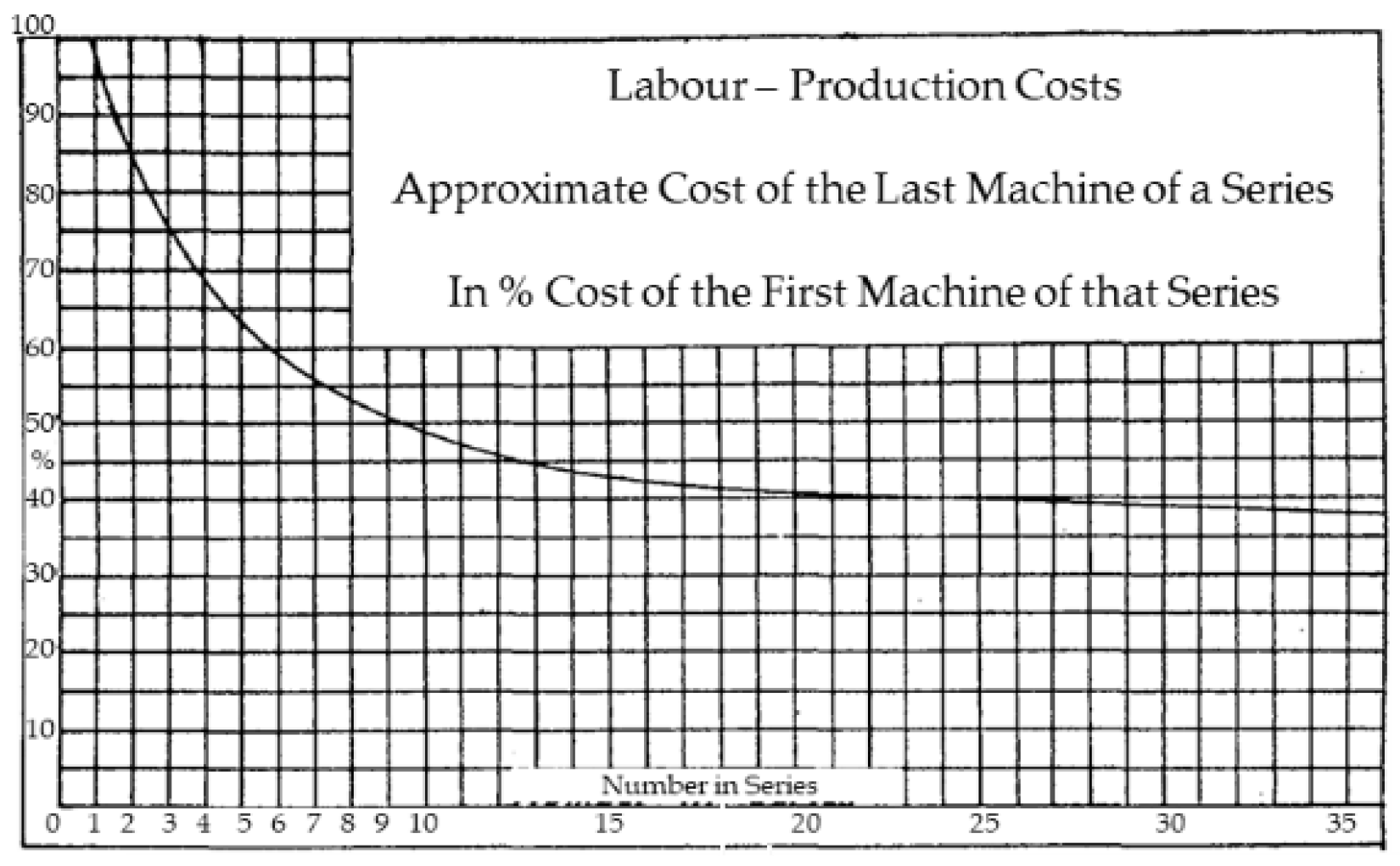
• Cumulative Average Learning Model—Developed in 1936 by Wright [10] who observed that after doubling the produced parts, the production time was reduced by a constant rate. Wright’s learning curve model offers its calculations based on the following Equation (1):

  $$\overline{y}=a{X}^{-b}$$

  (1)

  which represents the cumulative average cost or time of the first x unit, where A is the theoretical cost or time to produce the first unit, and b is the natural logarithm of the learning curve slope divided by the natural logarithm of 2. From Wright’s observations, the learning curve slope parameter should be 80% to approximate a bomber manufacturing process behaviour (see Figure 1). Multiple variations of his model were created afterwards, accounting for process-specific variables observed by other authors and parameters not considered in his initial model. Some of the more popular examples are the Stanford-B model, Crawford’s unit learning model, and Conaway & Schultz’s plateau model.

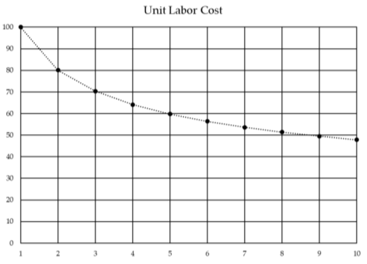
• Unit Learning Model—Developed in 1947 by Crawford [12], which base formula is the same as the cumulative average learning model from Wright [10], however, there is a difference in interpretation of the values where $\overline{y}$ represents the individual cost or time of unit x where the rest of the variables remain the same (see Figure 2).

These previous log-linear models as presented by Wright [10] and Crawford [12] had a main disadvantage in the long term; the learning rate would keep on reducing the estimated cycle time indefinitely, which prompted several other authors to explore and develop better fitting models to account for the reduced learning rate.

Adapted Log-Linear Models

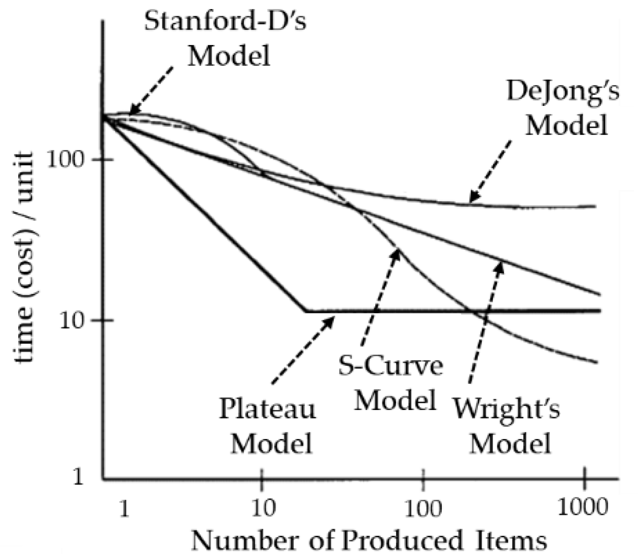
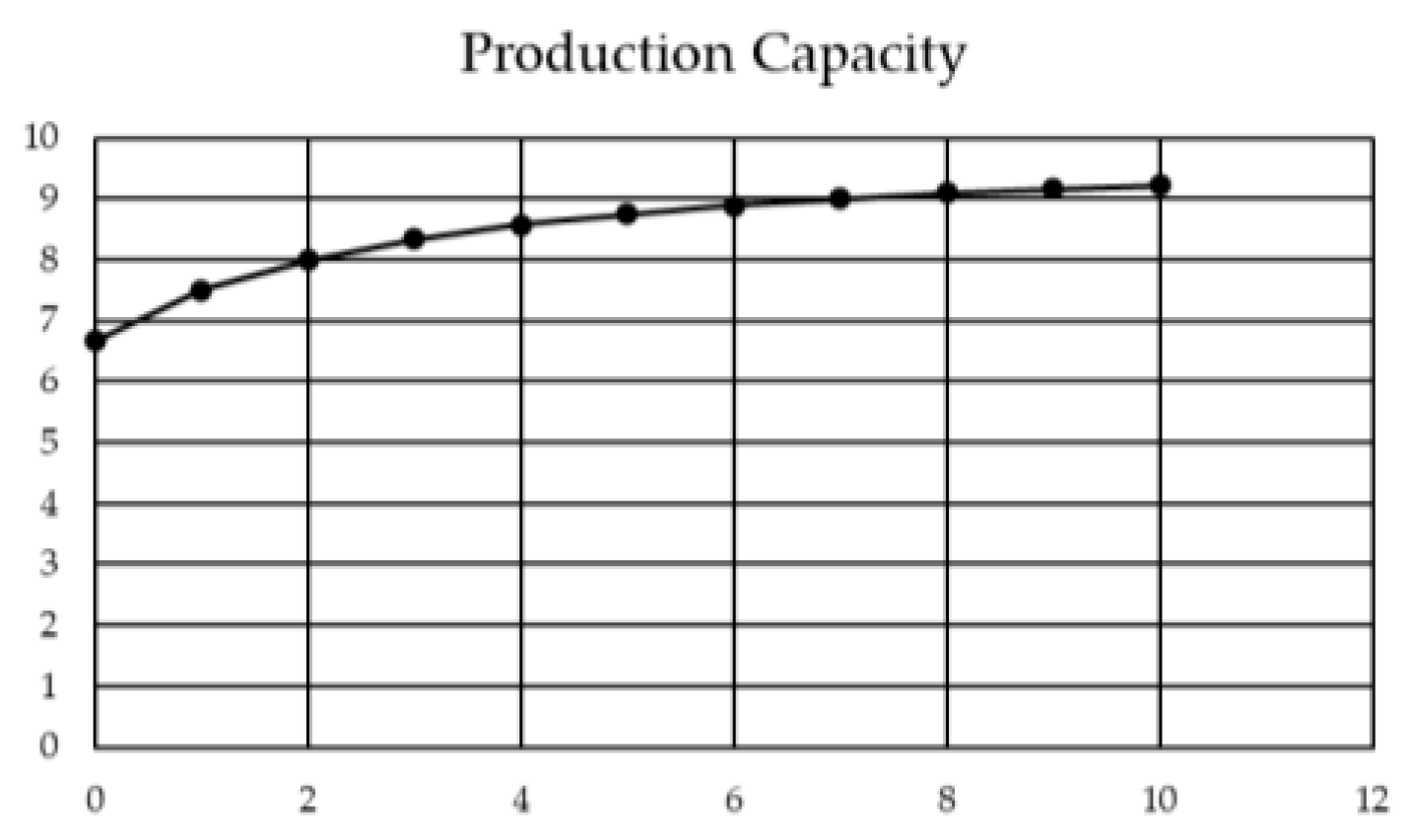
• Plateau Model—In 1957, Conaway & Schultz [13] first described the plateau effect in their learning curve model to account for the reduction in the learning rate. To account for this effect, the authors based their model on Wright’s learning curve [10], modifying it by adding a second process parameter c, which represents the standard time estimated from empirical data (the long-term value of the cycle time), thus generating a plateau on the learning curve on the value of c, via the Equation (2):

  $$\overline{y}=(A-c)x^{-b}+c$$

  (2)

  where the values of A, x, and b are the same as the ones found in Wright’s model [10] (see Figure 3). Another notable example of the plateau geometry model is presented by Yelle in 1979 [14], accounting for the limits a machine presents on the learning curve of an operator, meaning he/she cannot lower the cycle time below the standard operating time of a machine.

• Stanford-B Model—After World War II, the Stanford Research Institute was commissioned by the US Air Force to develop a new cost estimating learning curve for a process with previous similar production, meaning a previous workforce experience. To assess the presented requirement, the Institute developed the Stanford-B model, named after the additional B parameter, corresponding to the previous B number of units of experience, shifting the original log-linear along the time axis [15] (see Figure 3). To achieve this, the new learning curve model was expressed as Equation (3):

$$\overline{y}=A{(x+B)}^{-b}$$

(3)

• DeJong’s Model—DeJong realized in 1957 [16] that certain operations where machines were involved had a reduced learning effect on the operator, and a fraction of the cycle time came from the standard operation of the machine. He developed a model to assess this effect on burden-heavy operations with the mathematical modelling of Equation (4):

  $$\overline{y}=A[M+(1-M\left)x^{-b}\right]$$

  (4)

  where M represents the fraction of the work performed by a machine. When M = 1, meaning a total automated process, the learning effect becomes 0, leaving a constant work rate, and when M = 0 the model simply becomes Wright’s log-linear model [10] (see Figure 3).

• S-Curve Model—Named after the particular shape of the graph of the model [17], it is a combined form of both DeJong’s assessment of the machine involvement in the learning process [16] and Stanford-B’s previous experience effect [15]. Thus, the resulting model is Equation (5):

  $$\overline{y}=A[M+(1-M\left){(x+B)}^{-b}\right]$$

  (5)

  where the parameters keep the same meaning as in the origin model. The result is an S-shaped curve with a more precise but harder-to-estimate model of four parameters (see Figure 3).

Other adapted function models have been created following the base log-linear model of Wright [10] such as Levy’s Adapted Function [18] or Knecht’s [19] modification of Levy’s model [18]. Although these models are not usually discussed in the broader literature, it is to note that Levy’s Adapted Function [18] was presented as the first step towards an exponential model, the later Levy’s Adateed Function Model in the same article [18].

Derived from all the variations of the log-linear model, different models started adding new learning parameters, which lead to more complex mathematical models, mainly hyperbolic and exponential models to assess different particularities found in certain groups of work processes.

Exponential Models

To assess the diverse learning effects on workforce skills development, different exponential models were developed using the existing log-linear models as their foundation but adding a “damping” effect on their learning curves, thus an exponential behaviour. The main exponential models discussed in the scientific literature are:

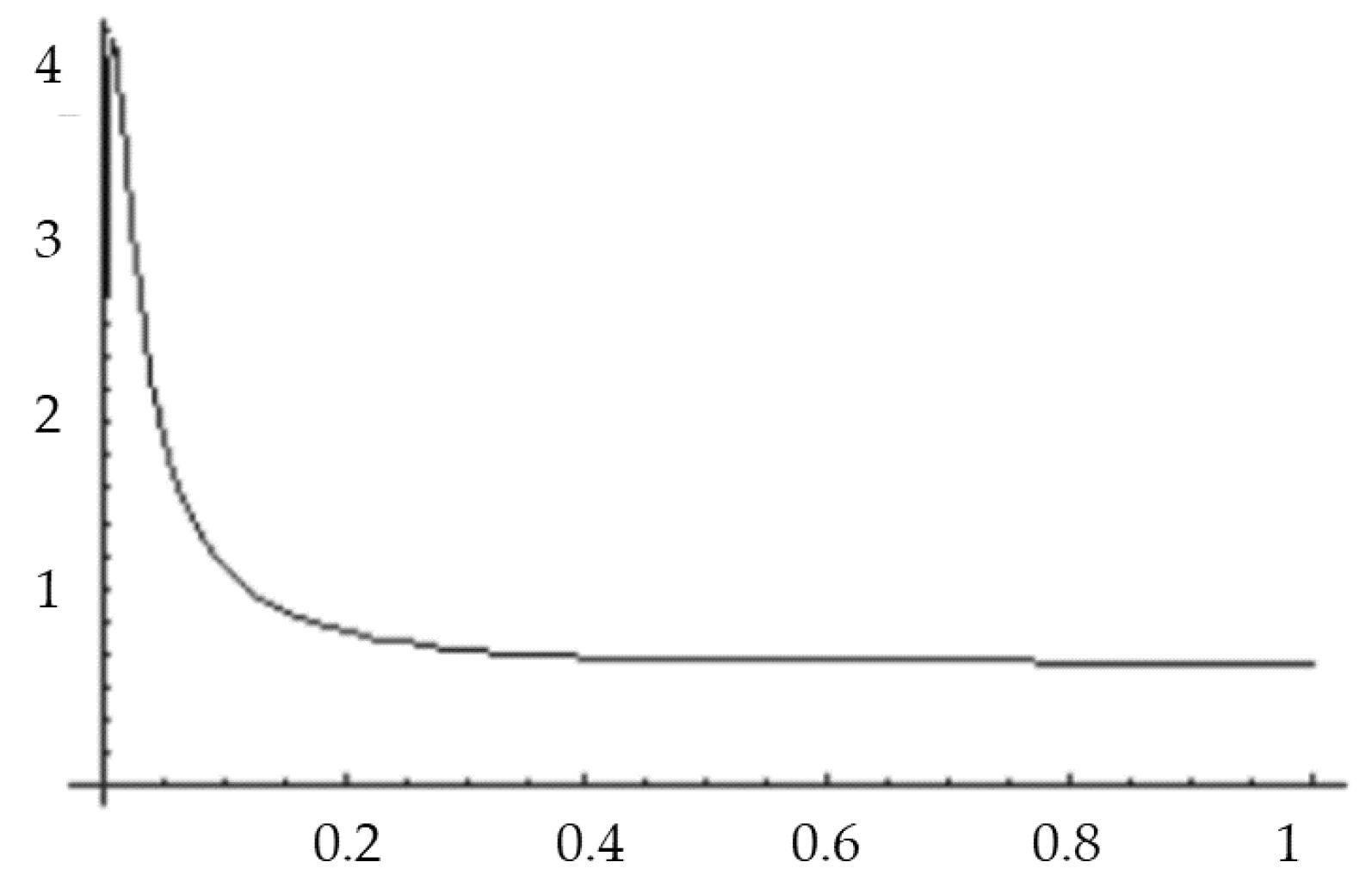
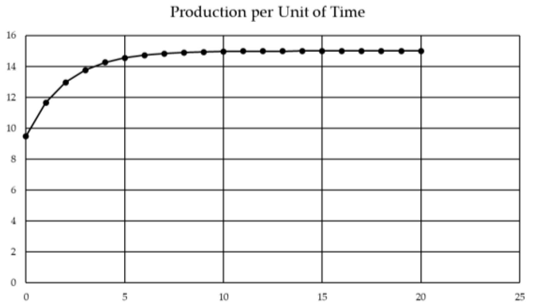
• Levy’s Adapted Function Model—From the adapted function model developed by Levy [18], the author added a parameter λ representing the speed at which the model approaches the maximum estimated throughput (P max). The resulting mathematical Equation (6):

  $$iP\left(x\right)=\left({1-e}^{\wedge }\right(-\lambda x\left)\right)(+(x^{\wedge }b/y\_1 \left)e^{\wedge }\right(-\lambda x)$$

  (6)

  where the variables b, x and y keep the same interpretation as in Wright’s model [10], being b the natural logarithm of the learning curve slope divided by the natural logarithm of two, x the current production unit in the lifecycle and y the initial cycle time of the process (see Figure 4).
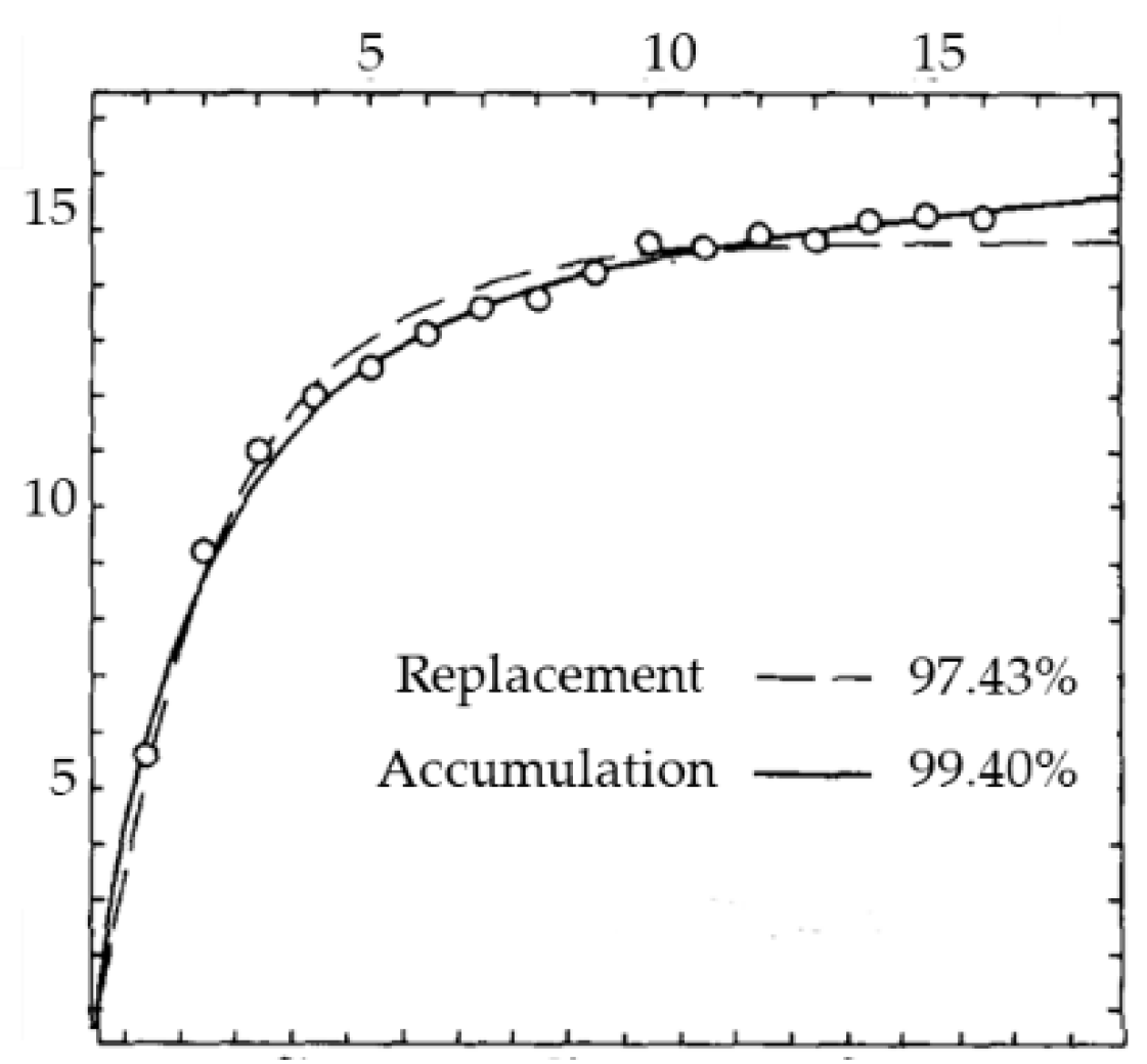
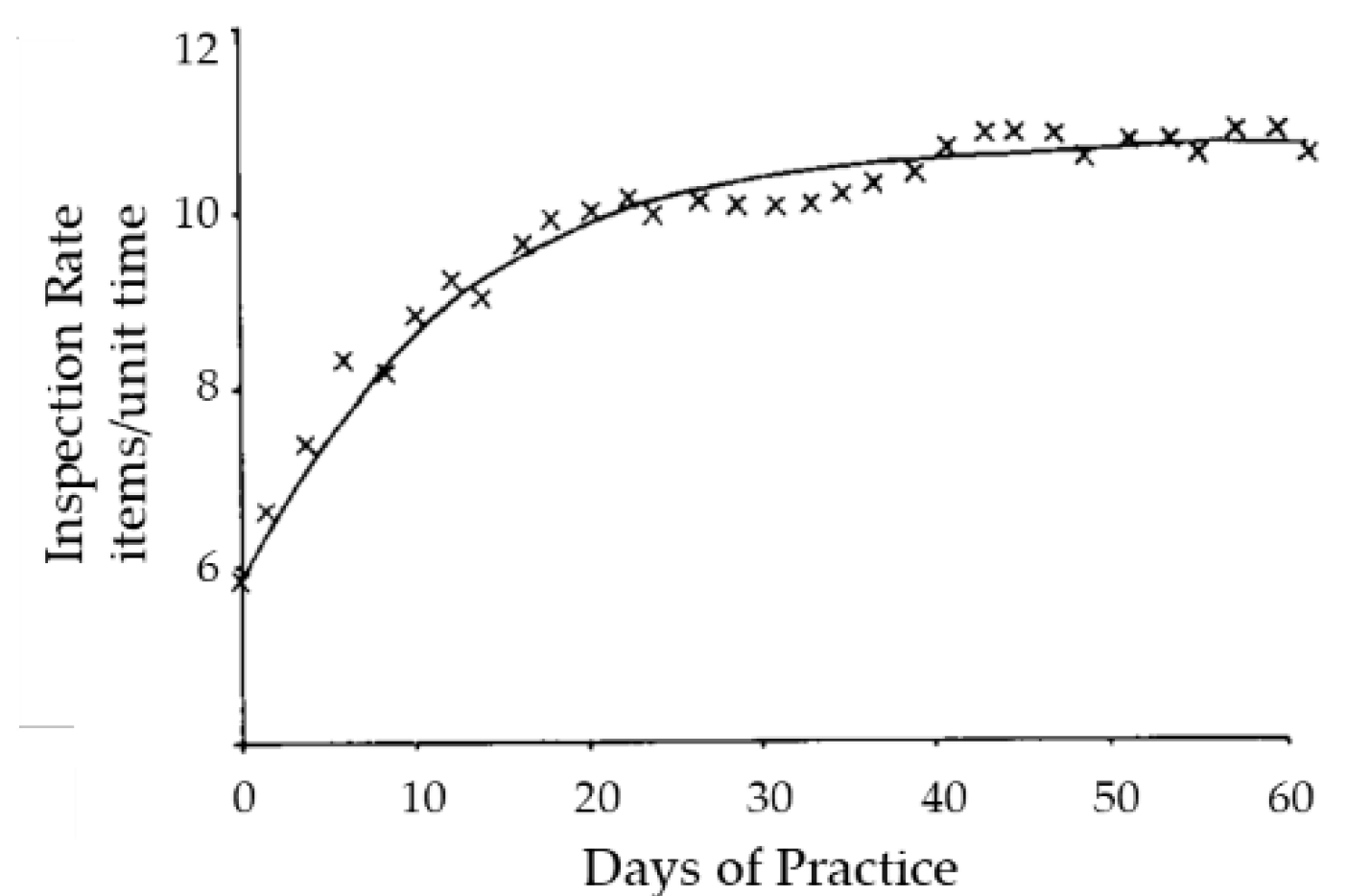
• Two and Three Parameter Models—Both models were proposed by Mazur & Hastie in 1978 [20], the Two Parameter model offers an approximation of the skill development behaviour in the workforce using two new parameters; k which represents the maximum throughput of a worker after the learning curve slope approaching zero, and the parameter r representing the learning rate in time units. The resulting Equation (7) is:

  $$y=k\left(1-e^{-\frac{x}{r}}\right)$$

  (7)

  After t developing the Two Parameter model, Mazur & Hastie [20] improved the fitting accuracy by adding a third parameter, p which corresponds to the worker’s prior experience, expressed in time units (see Figure 5). The mathematical Equation (8) for this variation is:

  $$y=k\left(1-e^{\frac{-\left(x+p\right)}{r}}\right)$$

  (8)

  The authors establish that their Three Parameter model has a good fit with operations where the operator has previous experience but performs poorly with operations that frequently require new and complex tasks (see Figure 6).
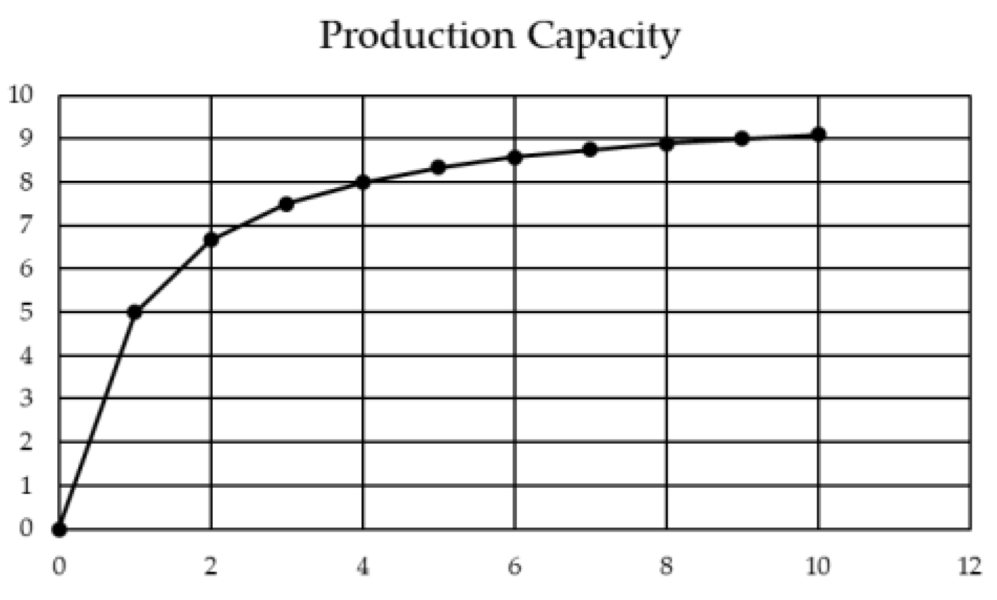
• Constant Time Model—In 1990, Towill [21] validated a similarly structured model to the Two Parameter model. He found that an exponential model with a starting constant value is better suited to estimate the learning curve of processes after the steepest learning curve period, meaning after they have adapted to a new task or job. The model’s mathematical Equation (9) is represented as:

  $$y=y_c+y_f\left(1-e^{-\frac{x}{\tau }}\right)$$

  (9)

  where y_c represents the worker’s initial performance, y_f is the highest achievable performance after learning, x remains the same as previous models (meaning how many units of experience the worker has), and τ is the time constant for a particular curve (see Figure 7).

Hyperbolic Models

Another group of models that came after the log-linear models were the hyperbolic models. These novel models have become relevant for the study and further advancement in recent years of learning curves due to their capacity of showing both the increase and decrease of cycle time due to the parameters they use to measure work performance. There is one main group of hyperbolic models developed by Mazur & Hastie in 1978 [20]. These are the Two and Three Parameter hyperbolic learning curve models, both of which have a similar mathematical formulation as the Two and Three Parameter exponential learning curve models, but these differentiate themselves by including a parameter p to assess the prior experience (see Figure 8). The resulting Two Parameter hyperbolic model Equation (10) is:

$$y=k\left(\frac{x}{x+r}\right)$$

(10)

where initially the parameter r refers to the total nonconforming units, x refers to the conforming units, and k refers to a constant production level. The Three Parameter hyperbolic model follows a similar Equation (11):

with the inclusion of the parameter p representing the previous units of experience (see Figure 9).

$$y=k\left(\frac{x+p}{x+p+r}\right)$$

(11)

One of the main topics of discussion in the scientific literature is the estimation of the parameters of the learning curves. In most of the case studies used to validate the previous models presented, the data was collected using work study techniques, or in some cases just approximations of the cycle times. Estimating the parameters allows a researcher to categorise previous runs or batches, and understand how similar processes learning curves will behave. However, multiple new data collection methods have arisen due to technological advancements in different areas (e.g., smart sensors). Combining the previous learning curve theories and current technological advancements could benefit all the different research areas where learning curves are being studied and applied.

Comparative Analysis of the Clusters of Learning Curve Models Revised

Table 1. Comparative analysis of the clusters of learning curve models revised.

Cluster	Advantages	Disadvantages
Traditional Log-Linear Models	A single parameter makes the estimation simpler. Due to their simplicity, they are commonly used in the industry.	Assume continuous learning, never reaching a plateau. Do not consider additional effects such as learning dampening.
Adapted Log-Linear Models	Consider additional effects such as burden-heavy operations and previous work experience. Most need a single learning parameter, making them easy to estimate.	Most still rely on the continuous learning assumption not achieving a learning plateau.
Exponential Models	Use a maximum achievable rate to the dampen effect of learning.	Due to their increased complexity and damping effect, most have two or three parameters making them harder to estimate.
Hyperbolic Models	Consider a simultaneous increase and decrease in the learning rate. Have a focus on quality calculations considering non-conforming and conforming units.	Due to their complexity, they include two or three parameters making them harder to estimate.

presents a comparative analysis of the advantages and disadvantages of the clusters of learning curve models revised in this state-of-the-art review.

3. State-of-the-Art Review Methodology

In this state-of-the-art review, the focus is on the use of learning curves in the manufacturing domain to understand the capacity of an operator to improve his/her assembly skills over time so that his/her work cycle time can be improved without compromising the process and its output quality as well as on the understanding of the technological advancements in data collection methods for labour intensive operations. Both objectives aimed to better comprehend if the advancements in both research areas (domains) could be integrated for the benefit of each other.

To identify, select, and analyse the sources of information relevant to this state-of-the-art review, the PRISMA 2020 updated guidelines as presented by Page et al. [22] were followed. Figure 10 shows the executed phases with the filters applied at each phase as the review was being conducted.

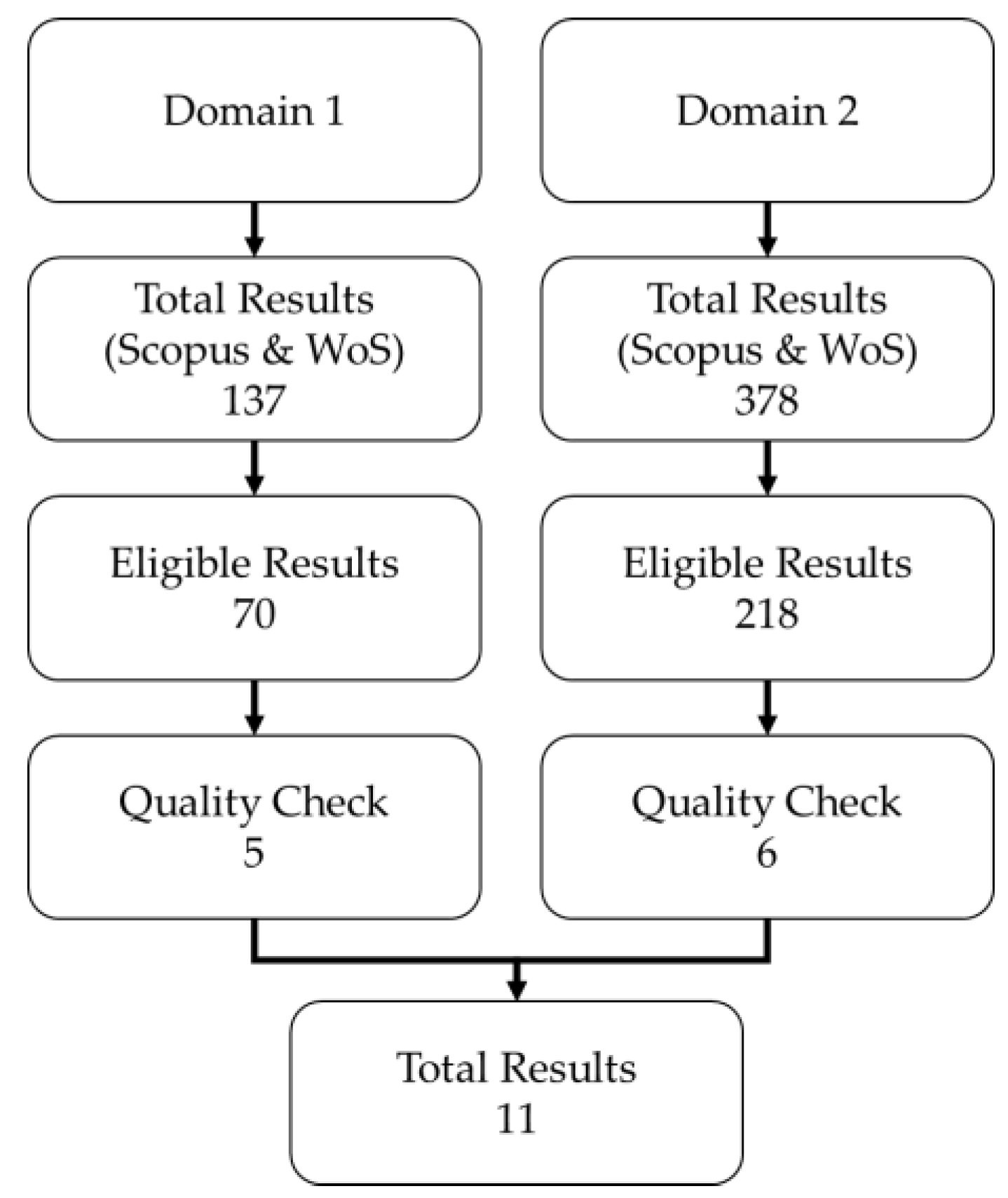
3.1. Search Strategy

The scientific databases that were selected for this state-of-the-art review are Scopus and Web of Science due to their high indexing level of engineering and sciences journals and international conference proceedings. The queries in the databases were done manually according to the keywords defined in the next subsection.

3.2. Keywords Selection

The authors proposed two sets of keywords based on the two main domains related to the research questions to be answered: (D1) workforce learning curve models and measurement methods, and (D2) data acquisition and monitoring technologies for human-based assembly operations. The selection was made by taking into account a broad set of words used commonly to describe this review’s desired area of interest.

Table 2. Keywords selection.

Domain	Keywords
D1. Workforce learning curves models and measurement methods (see RQ1 & RQ2)	Learning curves; Human factors; Throughput prediction; Standard times; Productivity
D2. Data acquisition and monitoring technologies for human-based assembly operations (see RQ3).	Monitoring; Assembly operations; Standard times; Human factors; Prediction; Manufacturing

shows the keywords selected for each domain of research. It is important to note that the keyword “prediction” was selected due to the similarity of use in scientific journal articles and conference papers not closely related to work studies but rather to productivity management and scheduling so it was evaluated as a synonym of application.

Some of the keywords overlap due to the need of making the queries more context-specific towards industrial engineering and manufacturing disciplines since for example learning curves may also refer to machine learning curves in the computer science discipline. Moreover, it is important to mention that even though the selection of keywords for this review was made trying to be as semantically broad as possible, different authors may use different terms to refer to similar concepts, and due to this some papers relevant to the area may not be included in this state-of-the-art review.

3.3. Query Construction and Execution

Given the selected keywords, one query stream was created applicable to each domain. The search string generated for each domain contains the keywords in multiple combinations relevant to the topic of this state-of-the-art review based on papers touching upon the topic of matter.

Table 3. Query string executed and initial results.

Query Stream	Domain	Results
(“standard times” AND “learning curve”) OR (“throughput prediction” AND “variability”) OR (“productivity” AND “learning curve” AND “prediction”) OR (“productivity” AND “human factor” AND “prediction”) OR (“productivity” AND “labor intensive” AND “prediction”)	D1	137
(“standard times” AND “variability” AND “monitoring”) OR (“monitoring” AND “human factors” AND “prediction”) OR (“labour intensive” AND “monitoring” AND “prediction”) OR (“labour intensive” AND “prediction” AND “variability” AND “manufacturing”) OR (“labor intensive” AND “prediction” AND “variability” AND “manufacturing”)	D2	378

shows the different combinations of keywords and the domain applicable to each as well as the initial results for the utilized query streams.

The presented number of results in Table 3 is the direct output number of their corresponding query in the selected databases, previous to any filters detailed in the next subsections. Needless to say, additional possible combinations of keywords could be used for supplementary query strings, however, the selected keywords combinations (strings) were decided to have in mind the scope and aims of this review, which are understanding the learning curve “prediction” models state-of-the-art and technologies available to acquire the data needed for supporting their “forecasts” for manual assembly operations.

3.4. Information Sources and Eligibility

Scopus and Web of Science databases were selected to search for relevant and up-to-date scientific literature due to their fast and high indexing efforts of engineering and sciences journals and international conference proceedings. Scopus was selected because based on a quick scanning of the pertinent literature for this state-of-the-art review, a large number of articles and papers related to learning curve studies have been indexed by this database, and Web of Science, on the other hand, was selected due to the indexed journals relating to applied sciences, such as the case of the main research topic at hand, since learning curves are by itself a practical application of theoretical and mathematical concepts such as “curve fitting”.

To filter the most relevant information sources for this state-of-the-art review, rather than a full literature review, the following filters were applied to the searches:

1.

Language: English—Due to being the main publishing language for the most important journals and international conference proceedings related to this research.

2.

Time-span: From 2017 to the current writing year (2022) looking to study the research domains state-of-the-art covered by this review.

3.

Article-type: Academic (peer-reviewed) journal articles and international conference papers; these last ones are given that international conference proceedings normally offer the most recent research results.

4.

Full keyword combination hit in an article: Title, keywords, or abstract.

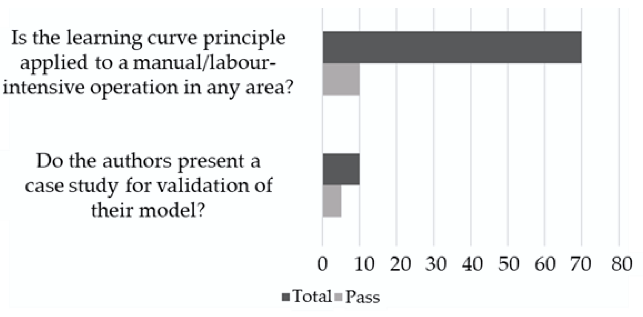
3.5. Quality Check

The following criteria were generated to select relevant journal articles and conference papers for this state-of-the-art review. These criteria (questions) allowed the authors to select the articles and papers with the most pertinent information to answer the research questions.

For Domain 1—Workforce learning curves models and measurement methods – the quality check criteria were:

• Is the learning curve principle applied to a manual/labour-intensive operation in any area?
• Do the authors present a case study to validate their model/research method?
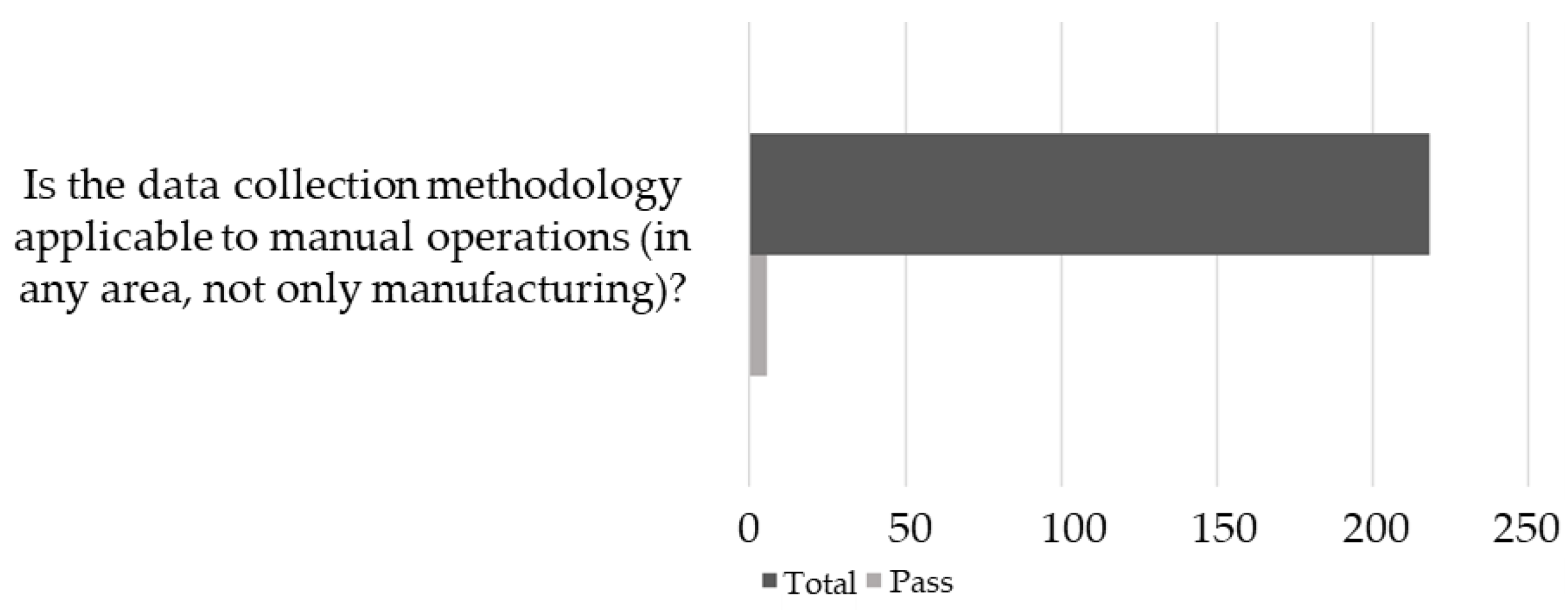
• For Domain 2—Data acquisition and monitoring technologies for human-based assembly operations—The quality criteria were:
• Is the data collection methodology applicable to manual operations (in any area, not only manufacturing)?

Though some papers from D1 address data collection methods due to their primary focus on “validating a learning curve model” these are classified as D1. Later in Section 5, their contributions to D2 are discussed in detail.

The results of each check and domain are presented in Figure 11 and Figure 12. Out of the initial 137 articles or papers for Domain 1, and 378 articles or papers for Domain 2, all the filters left 11 relevant articles and papers related to the incumbent topic for this state-of-the-art review.

To avoid selection bias in this phase of the PRISMA methodology, first, the authors worked independently during the quality check process to avoid influencing each other’s decisions, and then collaboratively to make a final selection of the articles and papers to be included in this review.

In the next section, the resulting 11 journal articles and conference papers will be presented, summarized, and discussed.

4. Results

This section was divided into two-level subsections to provide a concise description of the state-of-the-art findings per article/paper reviewed in chronological order of appearance in the scientific literature from the oldest to the newest. To keep the division of the two domains of study established, the results are presented separately in their respective domain subsection.

4.1. Domain 1: Workforce Learning Curves Models and Measurement Methods

The reviewed articles and papers in this domain subsection are related to workforce learning curve models, applied to different scenarios, and their different measurement methods for calculating and assessing the learning effect in manual operations (not only applicable to manufacturing as presented in the filters of Section 3).

4.1.1. Learning Curve Parameter Estimation beyond Traditional Statistics by Tilindis & Kleiza (2017)

This journal article by Tilindis & Kleiza [23] focuses on the parameter estimation of both Wright’s [10] and Crawford’s [12] learning curve models using limited production data by unit. To conduct this study, Tilindis & Kleiza proposed multiple estimation methods, namely: two-point, invariant, point-&-interval (just for Crawford’s model [12]), and two intervals. Moreover, to test and validate which estimation method produces a learning curve model (either in Wright’s [10] or Crawford’s [12] curves) that adjusts to real-life data, Tilindis & Kleiza [23] applied the methods to data obtained from a manual harness assembly process for the automotive industry. Furthermore, the reasoning behind utilizing simple, univariate models (C W) instead of more complex, multivariate ones is due to the limited data available, and the low production capacity available to run tests limited the ability of the researchers to test. The conclusions gathered from the experiment were that Wright’s learning curve model [10] presents a better fit to the real process behaviour when obtained through the invariant estimation method with enough fed data.

4.1.2. Application of Learning Curves in Operations Management Decisions by Tamás & Koltai (2019)

In this journal article by Tamás & Koltai [24], the authors present two reviews on learning curve topics within the scope of operations management decisions. The first review is on the development of learning curve models up to the year 2019, and the second review is on the learning effect on the calculation of the Economic Manufacturing Quantity (EMQ), which in traditional literature considers constant production rates [25]. Tamás & Koltai had the hypothesis that constant production rates are not applicable for new products, new processes, or long lifecycle ones. However, after reviewing different learning curve models and their validations, the authors concluded that utilizing the traditional Equation (12):

$$Q=\sqrt{\frac{2KD}{h\left(1-x\right)}}$$

(12)

To calculate the EMQ offers a more accurate and far simpler method in computational terms than introducing the learning curve effect. Next, Tamás & Koltai analyzed the effect of learning curves in break-even analysis for financial evaluation, where they conclude, that if the learning effect is ignored in processes where labour represents a large portion of production costs, the financial results could be underestimated, making a company lose focus on possible competitive opportunities. Finally, Tamás & Koltai, within the application of learning curves on assembly lines and the balancing of operations, concluded that traditional balancing is not enough when the learning effect is present.

4.1.3. A Machine Learning Approach to Predict Surgical Learning Curves by Gao et al. (2020)

Although this research work is not in the manufacturing domain, the novel approach used by Gao et al. [26] for predicting the learning curves of manual surgical operations could be well translated to manual assembly operations in a production line. In this journal article, Gao et al. utilize the “Kernel partial least squares” [27] machine learning technique to predict the learning curve features of a surgical operation through a non-linear transformation of the 10 first trials of a new operation/new subject using 13 inputs of learning curves based on Wright’s model [10], and the observations are then regressed to maximize their covariance. Moreover, to verify that the obtained learning curve data applies to multiple training environments, virtual and real training environments were used in the experiment, specifically the VBlaST-PT (consisting of Haptic devices to capture the hand movements of the surgeons and digitize them in a virtual environment) and the FLS Surgery Training Box (set of haptic devices to monitor and correct movements for surgery, similar to VBlaST-PT, but with physical surgery elements). Both are further described by the authors in the article. Furthermore, the conclusions of this study focused on the benefits of early identification of lack of training in some surgeons since the training and feedback systems proposed can be custom-tailored early on in the training.

One key feature to note is that this research work focuses on a single learning parameter like Wright’s model. Here Gao et al. name it “learning ability”, which captures the complexity of the learning process in the activity developed.

4.1.4. Cost Estimating Using a New Learning Curve Theory for Non-Constant Production Rates by Hogan et al. (2021)

In this journal article, Hogan et al. [28] begin the presentation of their research work by introducing two traditional learning curve models proposed by Wright in 1936 [10] and Crawford in 1947 [12] and their prediction values in the manufacturing domain. However, they immediately proceeded to explain the main disadvantage of using these two models that arises from having a “constant learning rate”, which means that these learning curve models do not consider a decline in human performance in the long-term that is normally caused by natural (human) forgetting, during production breaks, and/or by random factors (both external and internal) not planned by production [16]. Then, Hogan et al. proceed to detail five different decaying learning rate methods, which are more appropriate to the dynamics of the labour realities of the shop floor: (i) the plateau model [13], (ii) the Stanford-B model [15], (iii) the DeJong model [16], (iv) the S-Curve model [17], and (v) the Knecht’s upturn model [19].

The main research goal of Hogan et al. is to demonstrate how Boone et al.’s [29] model compares to other popular and/or traditional models for learning curve prediction models. Boone et al.’s [29] model Equation (13):

$$\overline{y}=A{x}^{\frac{b}{1+\frac{x}{c}}}$$

(13)

where the parameters keep the same value as Wright’s model [10] being A the initial cost of producing the first unit, b is the natural logarithm of the slope of the learning curve divided by the natural logarithm of two, and c a positive decay value affecting the slope of the learning curve along the time, keeping the number of units produced expressed as x. Given that Boone et al.’s learning curve model is relatively recent (published in 2021 [29]), Hogan et al. considered that further testing is required in real manufacturing environments, so they obtained more data from real manufacturing processes and compared Boone et al.’s prediction model [29] versus both Wright’s [10] and Crawford’s [12] models. The results showed that the accuracy of Boone et al.’s model [29] was statistically higher than the selected traditional models when sample sizes were large enough. Moreover, one caution of Hogan et al.’s research work, expressed by its authors, is that most of the data was gathered from production lots instead of unitary production data (single products), which should not have any effect on the study results but makes the findings not conclusive on whether Boone et al.’s model [29] is better when production data is unitary.

4.1.5. The Human Performance Impact on OEE in the Adoption of New Production Technologies by Di Luozzo et al. (2021)

In this journal article, Di Luozzo et al. [30] begin their study by acknowledging the impact of human performance, process configuration, and technical features on the ramp-up phase of the adoption of a new process or technology on an automated or semi-automated production process. Here, Di Luozzo et al. refer to Wright’s [10] learning curve model to consider it in the learning of maintenance operations and the time that it takes a maintenance technician to perform these. Thus, Di Luozzo et al. propose two new methods for OEE (Overall Equipment Effectiveness) calculation, making it easier to separate and identify the errors of the mentioned factors during a production ramp-up period. They tested their new OEE calculation methods with a case study that involved the implementation of a new semi-automated packaging process in a logistics company, which allowed them to demonstrate that having several more factors for an OEE calculation, helps to better visualize the training plans for the operators to accelerate the ramp-up production period.

As depicted in

Table 4. Comparison of Domain 1—Reviewed journal articles and conference papers for learning curve models.

Article/Paper	Described Models	Technique	Data Collection Method	Application Area	Contribution	Areas of Opportunity
Section 4.1.1 Tilindis & Kleiza (2017) [23]	Wright’s [10] Crawford’s [12]	Estimation via: Two Point, Invariant Point, Interval, and Two Intervals	Not Specified	Manual Harness Assembly	Achieved the estimation of curve parameters using limited data	Only traditional log-linear models were tested
Section 4.1.2 Tamás & Koltai (2019) [24]	Wright’s [10] Crawford’s [12] Plateau [13] Standford-B [15] DeJong’s [16] S-Curve [17] Two & Three Parameter Hyperbolic [20]	None	None	Economic Manufacturing Quantity (EMQ) [24] Break-Even Financial Analysis Balancing of Operations	Multiple application areas are reviewed with a deep comparison between the validation models reviewed by the authors	Applications are not evaluated with Exponential Models
Section 4.1.3 Gao et al. (2020) [26]	Wright’s [10]	Machine Learning (Kernel PartialLeast Squares) [26]	VBlaST & FLS Surgery Training Box	Surgery Training	Prediction of learning curves was achieved using the first few points in the proposed Machine Learning Algorithm	Only Wright’s model was tested
Section 4.1.4 Hogan et al. (2021) [28]	Boone et al.’s [29]	Data Fit (MAPE Evaluation)	Batch Production Time Reports	Military Plane Assembly	Demonstrated Boone’s model fits better to the presented study case	Only traditional log-linear models were tested
Section 4.1.5 Di Luozzo et al. (2021) [30]	Wright’s [10]	OEE Calculation Integration	Maintenance DurationReports	Packaging Semi-Automatic Process Maintenance	Not only learning curve is assessed, but many other human factors in a singl calculation	Learning curve is only considered for maintenance, not for a mainmanual activity

, only one new learning curve model has appeared in recent years (2021) in the scientific literature: Boone et al.’s model [29]. This “new” model integrates the previous knowledge from the different classic models discussed in this review. Furthermore, one major trend that has been identified in this state-of-the-art review of learning curve models is their growing application beyond manufacturing in the areas like Finance/Economics [25] and Health [26]. Moreover, new ways of estimating learning curve parameters are being observed in the state-of-the-art such as with the support of machine learning approaches [26] that in an emerging data-rich era might turn out to be the next step in learning curve measurements/estimations in different areas, including manufacturing.

4.2. Domain 2: Data Acquisition and Monitoring Technologies for Human-Based Assembly Operations

The presented journal articles and conference papers are related to data collection methods and monitoring tools applicable to manual operations. These can be applied to cycle time monitoring, but are not limited to it, since other technologies to monitor additional factors could be adapted to monitor time. The main focus of this subsection is to understand what are the latest advancements in general data acquisition and monitoring technologies.

4.2.1. Human Factor Analyzer for Work Measurements of Manual Manufacturing and Assembly Processes by Faccio et al. (2019)

The purpose of this journal paper by Faccio et al. [31] is to present and demonstrate the function of a “human factor analyzer”, a combination of software and hardware solution components consisting of a set of motion tracking cameras similar to the ones used in motion tracking for animated films, and a software program that digitizes the tracked operator movements to monitor his/her manual manufacturing and assembly process-tasks and gathered data related his/her movements’ time, speed, and reach. Faccio et al. have proposed this work measurement model since traditional measuring methods are often expensive, both in time and resources, and the reliability of the data depends on the skill and repeatability of the person responsible for the measurements. Faccio et al. first tested their proposed human factor analyzer in a lab environment, and later in an industrial environment, an Italian welding factory containing a process mainly dependent on human operators (i.e., welders), both of which demonstrate the easiness and simplification of high-quality data collection.

4.2.2. Continuous Measurement of Muscle Fatigue Using Wearable Sensors during Light Manual Operations by Fu et al. (2019)

Fu et al. [32], in their conference paper, address the muscle fatigue measure and management in real-time by using surface Electromyography (sEMG) sensors. The first topic they cover is the selection of the type of sensors, given they found common sEMG sensors to be heavy and stationary, they chose wearbands with wireless capabilities to monitor the fatigue. Another interesting approach from the authors is that, as mentioned by them, previous studies measured the signal during work breaks, and not in real-time during the operation during the production day. To validate if any correlation existed between perceived fatigue of the operator with real fatigue measured with the sEMG, the authors used Borg Rating of Perceived Exertion [33] where twelve operators rated their fatigue on different parts of the arm as well as using the sensors to objectively measure their fatigue. The results showed no correlation between the two variables, which the authors attribute to different possible psychological reasons that are not assessed in the sensor measurement. However, they also concluded the sEMG sensors offer a reliable way to measure physical fatigue that could help manage fatigue with additional breaks to optimize production and reduce health problems for operators.

4.2.3. Exploring the Potential of Operator 4.0 Interface and Monitoring by Peruzzini et al. (2020)

This journal article by Peruzzini et al. [34] proposes a human-centric digital performance measurement application, pertinent to the Industry 4.0 manufacturing framework, based on different data collection methods and devices for shop floor workers’ performance, actions, and reactions monitoring with the final objective of improving the overall production performance. The human-centric application consists of different performance measurement devices such as smart glasses to monitor eye gaze and pupil dilatation to monitor the operator’s interaction with devices and interfaces, wearable sensors to measure the operator’s health vitals, a bio-harness to measure the angle of the back of the operator, and a motion tracking system to digitize the operator body postures for proper work ergonomics, and a digital human modelling software to identify non-ergonomic movements. The research work revolves around generating ideal human-centric workstation designs based on the data collected. Peruzzini et al. tested their monitoring application on a case study of a manual assembly of air cabins of tractors. Using the data collected, they were able to find and improve activities that were not economical or efficient.

4.2.4. Human Digital Twin for Fitness Management by Barricelli et al. (2020)

This journal article by Barricelli et al. [35] focuses on the creation of a digital twin system to monitor vitals and relevant measurements of an athlete using “SmartFit”, a previously developed tool to capture said measurements. However, the main point of the article is the introduction of machine learning techniques to further the reach of “SmartFit”, where the authors propose a KNN imputation method and classifiers to generate performance forecasts for the athletes based on multiple predictors (i.e., calories consumed, speed, etc.) and generate suggestions to increase their performance, such as increasing calories or reducing speeds. Finally, the authors test their model with real athletes and validate that the presented application functions as expected.

4.2.5. A Multi-Sensor Approach for Digital Twins of Manual Assembly and Commissioning by Rebmann et al. (2020)

In the conference paper presented by Rebmann et al. [36], the authors focus on creating a digital monitoring system, and an aiding system based on the monitored data, which allows the operator to identify potential errors and available options in a manual process. To design and test their system, the authors use a manual operation consisting of multiple scenarios (i.e., inventory, assembly, and pickup stations) where the actions that the operator can perform are exclusive to each station. One of the main points of the paper is how, instead of constantly monitoring the movements of the operator in search of any specific movement related to any of the operations, the authors use what they call a “search approach”, which first validates the position of the operator and instead of looking for every possible action the operator could be doing, possible actions are filtered according to the current station, so only a certain quantity of actions are looked for at any given time. To achieve this, the proposed system is fed via a headset used by the operator as well as sensors on each of the stations to validate the possible actions, for example, picking something up that is on stock in the inventory station. The authors conclude that integrating information from different sensors allows each other to complement their capabilities and overcome their shortcomings while improving the performance of the operator and reducing the errors they can incur.

4.2.6. Parametrization of Manual Work in Automotive Assembly for Wearable Force Sensing by Kerner et al. (2021)

In this journal article by Kerner et al. [37], the researchers identify the need to parameterize a manual operation since having additional numerical data from something considered to be skill-based would help apply process control through statistical methods. The operation analysed is a hose assembly process, where the operator applies a sheer force in multiple stages. The authors developed a sensor inside the glove used by the operator that allowed them to measure precisely the force applied. Though it was not considered to estimate a learning curve, the methodology of how they analysed the operation to create a “method” to collect data could apply to other processes.

Even though most of the data collection systems presented are not fully implemented for manual operations tracking in an industrial setting, researchers are starting to look into ways of incorporating such human-based operations into Industry 4.0 environments. Moreover, currently, the focus is on improving the workstations and making them more ergonomic, the most recent papers (see

Table 5. Comparison of Domain 2 – Reviewed journal articles and conference papers for data collection methods.

Article/Paper	Data Collection Method	Monitored Data	Software	Application	Focus
Section 4.2.1 Faccio et al. (2019) [31]	Motion Tracking Depth Cameras	Joint Position, Joint Movements, Picking Duration and Frequency, and Travel Distance	Human Factor Analyzer (Proprietary)	Laboratory Production Setting for Picking Operation	Ergonomics, and Workstation Design
Section 4.2.2 Fu et al.(2019) [32]	Surface Electromyography Armbands	EMG Muscle Signals	None	Manual Assembly of Electrical Products	Fatigue Management
Section 4.2.3 Peruzzini et al. (2020) [34]	Eye Tracking System, Vitals Monitoring Wearable Sensor, Personal Video Camera, and Motion Tracking Cameras	Eye Gaze & Pupil Dilatation, Heart Rate, Breathing Rate, Temperature, Posture Angle, Ergonomic Scores, and Human Positions, Postures and Movements	Human Digital Modelling, and Motion Tracking Digitalization	Manual Assembly of Tractor’s Air Filter	Ergonomics, and Error-Proofing (Quality)
Section 4.2.4 Baricelli et al. (2020) [35]	Wristband Tracker	Nutritional Income, Daily User Activity, Duration and Quality of Sleep, and User’s Mood	Mood Tracking App, and Nutritional Tracking App	Fitness	User Feedback Loop for Improvement
Section 4.2.5 Rebmann et al. (2020) [36]	Inventory Weight Sensor, and Head Mounted Display Lenses	Material Handling Tracking	Image Based Scenery Classification	Laboratory Assembly Environment	Error-Proofing
Section 4.2.6 Kerner et al. (2021) [37]	Proprietary Shear Force Sensor	Manual Shear Force	None	Manual Hose Connections	Manual Operation Parametrization

) show a trend of aiding the operator to improve and even parametrize operations that previously were thought to be skill correlated [36], making it simpler to transfer knowledge and even find hidden parameters on his/her operations.

5. Discussion

After studying the journal articles and conference papers selected for this state-of-the-art review, in this section, a discussion is open to answer the original research questions presented by this work and for establishing possible areas for further research. It is worth mentioning that during this state-of-the-art review, three “literature reviews” were found in the scientific body of knowledge on learning curves. These reviews were excluded from the results presented in Section 4 since their focus was more on providing a retrospective analysis of the learning curves literary corpus rather than addressing its current research matters and future directions as intended by this “state-of-the-art review”. Nevertheless, a summary of the highlights of these three literature reviews found is discussed next.

Anzanello & Foglliato [11] presented in the year 2011 a literature review on applications, validations, and modifications to existing learning curve models to provide a theoretical background of these to the scientific community. Eight years later, Glock et al. [38] in the year 2019 offered a similar literature review, updating the work of Arizanello & Foglliato [11] once again with a retrospective vision. Later in the same year, 2019, Tamás & Kolte [24] also presented a literature review on the applications of learning curves but once again the focus was on the past and present rather than the future.

In the following subsections, each research question will be discussed in order.

RQ1. What Calculation Methods for Estimating the Learning Curve of a Worker Exist in the Recent Scientific Literature?

As demonstrated by the journal articles and conference papers reviewed, new learning curve models are starting to emerge. These models deliver higher complexity, considering decreasing learning rates, making these models multivariate models. This review shows that these models are more precise than previous models though they are harder to estimate. These new learning curve models, still tested with real-life data, are yet to be implemented for long-term parameterization in industry settings.

Advancements in the learning curves field have emerged, such as Boone et al.’s model [29], which considers a decaying learning rate with each unit produced. The authors [29] were able to show that their improved model is relatively better than the traditional univariate models proposed by Wright [10] and Crawford [12], making it a new possible model for future references such as the traditional models of Stanford-B [15], DeJong´s [16], and S-Curve [17].

Also, other authors have addressed the learning curve in new ways, such as including it in the OEE calculation method [30]. The main limitation to the approach that these authors took is that they only addressed the learning of human factors in the maintenance activity and not as part of the main production process, meaning the calculation is mainly affected by the “availability” component of the OEE, were, if considering the human factor for a manual operation instead of a semi-automated, the effects would be seen on the performance component.

However, parametrizing these learning curves is of uttermost importance since the parameters on any model are what characterize the curve and allow it to be studied. To conduct this, the main breakthrough, although not in manufacturing is the combination of machine learning with learning curves to estimate their parameters [26], which helps predict the learning curve from the first few tries to improve training programs. The adaptation of this method to other environments, such as manufacturing, testing additional learning curves could be further developed.

RQ2. What Other Usages Are Manufacturing Enterprises Giving the Modern Learning Curve Prediction Models According to the Recent Scientific Literature?

The main point of this discussion is to understand how real-time data is being used for the learning curve calculations and is in this regard that most papers provide an advancement on the state-of-the-art on learning curves. First of all, Gao et al. [26] propose a machine learning approach to predict traditional learning curves with the first few data points of a surgeon. This approach considers real-time data from training boxes and VR simulations, which are then processed and analysed by a KNN imputation algorithm [27]. The benefits presented by such an approach include identifying early training opportunities for surgeons to improve their learning curves. Though the application is not directly involved with manufacturing, the approach could be well applied and carried over to the industry.

Tilindis et al. [23] have a similar goal, to estimate traditional learning curves with as few points as possible, however, their approach leans towards iterative predictions using different methods, in the end resulting in the approximation of the real performance evolution through Wright’s learning curve with Invariant approximation method.

Baricelli [35] goes a step further, by not only predicting the learning curve, but generating an algorithm capable of generating suggestions to improve the learning curve based on the Kernel imputation method, using multiple linear regressions to predict the effect of changing one or more predictor variables, in the application case, calorie intake and speeds, and presenting these to the final user.

It is important to mention that this discussion is framed and limited to the scope of the learning curve models and data collection methods state-of-the-art since this research work objective is to address the latest advancements in both domains.

RQ3. What Data Collection and Monitoring Technologies Exist to Automatically Acquire the Data Needed to Create and Continuously Update the Learning Curve of an Assembly Operator?

As presented by Faccio [31] and Peruzzini et al. [34], a highly detailed digitalization of the human operator in the production line is helpful to gather specific and precise operations data, both to improve workstations taking into account the human anatomy and positions and to track and monitor the performance of movements and interactions. Both of these approaches collect massive data sets from single operations or operators. However, no journal articles or conference papers deal with the cost of implementing these solutions, which in the best case is affordable for one workstation, but makes it unsustainable for production lines with multiple operators in a line. Another point of discussion is how intrusive these sensors and tracking tools are, if not directly with the activity performed, such as interference in the movement, at least how hard is for the operator to put on and set up the whole sensor setup.

Baricelli [35] in his paper proposes tracking vitals through smart wearables, and even though the application of the paper is not directed to manufacturing, the detail obtained from the wearable proposed could provide valuable information regarding operator work conditions such as stress levels, heartbeat, and movement speed. However, this technology would have to be paired with a gyroscopic tracking device to identify exactly in which movement vitals change.

In the paper by Gao et al. [26] data collection is done in training boxes, both virtual and physical for surgeon operations. In manufacturing, plants usually have training grounds for their new operators, before moving them to a real environment, so similar data collection could be performed. However, one condition for this method is that it can only be applied to a pre-manufacturing area, meaning only to training conditions. This, however, can in turn be used similarly to the application Gao et al. journal article has, improving the operators’ training.

A simpler method, such as scale sensors mentioned in the article by Rebmann et al. [36], though useful for monitoring material picking, could hardly be applied by itself to predict learning curves. One main point of all papers is trying to have a human-centric approach when designing the capture systems, most of them using wearables or tracking systems focused on the operator. Another approach to follow could be the one followed by Kerner et al. [37] by creating human monitoring sensors on parameters not considered measurable in a previous state by using simpler sensors such as the shear force sensor presented by them.

6. Conclusions and Further Research

In this state-of-the-art review of the learning curves body of knowledge, two main topics were touched upon. First of all, the learning curve models, applications, and estimation methods achieved in applicable environments in recent years. Though not many new models have been developed (for this review only Boone et al.’s model [29] was found) the application and the reach of integration with estimation methods through mathematical [23] and machine learning [26] approaches, and the integration into the known concept of OEE (Overall Equipment Effectiveness) [30] are currently growing. Improving upon and even combining the methods of each of the journal articles and conference papers could contribute to even more precise results in the prediction of learning curves. In the case of Boone et al.’s model [29], having a similar approach that Gao et al. [26] had with Wright’s model [10] to parametrize it with machine learning, could bring forward both the model and the prediction accuracy. Applying Boone et al.’s model [29] to different applications, such as the ones found by Tamás & Koltai [24] to understand which scenarios using Boone et al.’s model [29] is more precise but also computationally comparable to traditional models could be of help for multiple areas of study.

Another area reviewed was the data collection methods. In an age where data is becoming more and more relevant with the rise of Industry 4.0 or Smart Manufacturing, measuring, monitoring, and processing data obtained from manual operations could be the next big step to a human-centred process design. In the current review, there were multiple systems identified, not only for the manufacturing sector but for general monitoring. It is important to note that the centre of the current researchers is improving working conditions and enhancing the capabilities of the operator, giving them feedback on the operations being carried out, moving forward with the concept associated with Industry 5.0, which evolving from Industry 4.0, represents a human-centred approach towards integrating technology to aid humans [39].

Integrating the two concepts, i.e., learning curve models and data collection methods, results in a potential research area, where learning curves could be analyzed and predicted in real-time using data obtained from any collection method, fed into a system and processed into different applications. In this research, mainly, four different integrated research points were identified, concerning the different papers reviewed. First of all, the data collection methods are an important factor to monitor and gather data from operators. Next, the learning curves, either the newest methods such as Boone et al.´s [29] or classical models such as Wright’s [10] or Crawford’s [12] to understand the increase in skill of operators. The parameter estimation method is another critical field, with recent papers utilizing methods such as point estimation methods [23] and machine learning [26] to process the gathered data, and approximate the learning curve parameters to better predict the performance of operators in the long term. Finally, the output or application of the result of the learning curve, meaning how the prediction of the performance could be used to benefit the operator, the organization or the process in an integrated way. In the literature reviewed, examples such as a feedback loop to improve human performance [35] or fatigue management in an operation [32] were found. In Figure 13, these four areas and their interaction are presented in a graphical format.

Further investigation will be carried out on the different components of the proposed conceptual research framework (see Figure 13) in the form of literature reviews for specific topics such as data collection and learning curve estimation methods that could offer good feasibility for their implementation in real manufacturing environments. Finally, using the manufacturing background found in the current literature as an initial base, and the current trend towards estimating the learning curves using “mixed” methods in this state-of-the-art review, the next research steps will focus on using these combined methods to predict the production performance of workers affected by the learning curve effect to aid the scheduling of production line in the long term.

References

- Gölzer, P.; Fritzsche, A. Data-driven Operations Management: Organisational Implications of the Digital Transformation in Industrial Practice. Prod. Plan. Control 2017, 28, 1332–1343. [Google Scholar] [CrossRef]
- Mittal, S.; Kahn, M.; Romero, D.; Wuest, T. Smart Manufacturing: Characteristics, Technologies and Enabling Factors. J. Eng. Manuf. 2019, 233, 1342–1361. [Google Scholar] [CrossRef]
- Wuest, T.; Weimer, D.; Irgens, C.; Thoben, K.-D. Machine Learning in Manufacturing: Advantages, Challenges, and Applications. Prod. Manuf. Res. 2016, 4, 23–45. [Google Scholar] [CrossRef]
- Hogan, D.W. An Analysis of Learning Curve Theory & Diminishing Rates of Learning. Master’s Thesis, Air Force Institute of Technology, Wright-Patterson AFB, OH, USA, 2020; p. 3607. [Google Scholar]
- Ohlig, J.; Hellebrandt, T.; Poetters, P.; Heine, I.; Schmitt, R.H.; Leyendecker, B. Human-centered Performance Management in Manual Assembly. Procedia CIRP 2021, 97, 418–422. [Google Scholar] [CrossRef]
- Andrianakos, G.; Dimitropoulos, N.; Michalos, G.; Makris, S. An Approach for Monitoring the Execution of Human-based Assembly Operations using Machine Learning. Procedia CIRP 2019, 86, 198–203. [Google Scholar] [CrossRef]
- Ebbinghaus, H. Memory: A Contribution to Experimental Psychology; Ruger, H.A.; Bussenius, C.E., Translators; Teachers College Press: New York, NY, USA, 1913. [Google Scholar]
- Yelle, L.E. The Learning Curve: Historical Review and Comprehensive Survey. Decis. Sci. 1979, 10, 302–328. [Google Scholar] [CrossRef]
- Swift, K.G.; Booker, J.D. Manufacturing Process Selection Handbook; Butterworth-Heinemann: Oxford, UK, 2013. [Google Scholar]
- Wright, T.P. Factors Affecting the Cost of Airplanes. J. Aeronaut. Sci. 1936, 3, 122–128. [Google Scholar] [CrossRef]
- Anzanello, M.J.; Fogliatto, F.S. Learning Curve Models and Applications: Literature Review and Research Directions. Int. J. Ind. 2011, 41, 573–583. [Google Scholar] [CrossRef]
- Crawford, J.R. Learning Curve, Ship Curve, Ratios, Related Data; Lockheed Aircraft Corporation: Burbank, CA, USA, 1944. [Google Scholar]
- Conway, R.; Schultz, R. The Manufacturing Progress Function. J. Ind. Eng. 1959, 10, 39–53. [Google Scholar]
- Yelle, L.E. Technological Forecasting: A Learning Curve Approach. Ind. Mark. Manag. 1976, 5, 147–154. [Google Scholar] [CrossRef]
- Baloff, N. Manufacturing Startup: A Model. Dissertation, Stanford University, Redwood City, CA, USA, 1963. [Google Scholar]
- DeJong, J.R. The Effects of Increasing Skill on Cycle Time and Its Consequences for Time Standards. Ergonomics 1957, 1, 51–60. [Google Scholar] [CrossRef]
- Carlson, J.G.H. Cubic Learning Curves—Precision Tool for Labor Estimating. Manuf. Eng. Manag. 1973, 5, 22–25. [Google Scholar]
- Levy, F.K. Adaption in the Production Process. Manag. Sci. 1965, 6, B136–B154. [Google Scholar] [CrossRef]
- Knecht, G.R. Costing, Technological Growth and Generalized Learning Curves. J. Oper. Res. Soc. 1974, 3, 487–491. [Google Scholar] [CrossRef]
- Mazur, J.E.; Hastie, R. Learning as Accumulation: A Reexamination of the Learning Curve. Psychol. Bull. 1978, 6, 1256. [Google Scholar] [CrossRef]
- Towill, D.R. Forecasting Learning Curves. Int. J. Forecast. 1990, 1, 25–38. [Google Scholar] [CrossRef]
- Page, M.J.; McKenzie, J.E.; Bossuyt, P.M.; Boutron, I.; Hoffmann, T.C.; Mulrow, C.D.; Shamseer, L.; Tetzlaff, J.M.; Akl, E.A.; Brennan, S.E.; et al. The PRISMA 2020 Statement: An Updated Guideline for Reporting Systematic Reviews. Res. Methods Report. 2021, 327, 71. [Google Scholar]
- Tilindis, J.; Kleiza, V. Learning Curve Parameter Estimation beyond Traditional Statistics. Appl. Math. Model. 2017, 45, 768–783. [Google Scholar] [CrossRef]
- Tamás, A.; Koltai, T. Application of Learning Curves in Operations Management Decisions. Period. Polytech. Soc. Manag. Sci. 2019, 1, 81–90. [Google Scholar] [CrossRef]
- Jaber, M.Y.; Bonney, M. The Economic Manufacture/Order Quantity (EMQ/EOQ) and the Learning Curve: Past, Present, and Future. Int. J. Prod. Econ. 1999, 59, 93–102. [Google Scholar] [CrossRef]
- Gao, Y.; Kruger, U.; Intes, X.; Schwaitzberg, S.; De, S. A Machine Learning Approach to Predict Surgical Learning Curves. Surgery 2020, 167, 321–327. [Google Scholar] [CrossRef] [PubMed]
- Kim, K.; Lee, J.M.; Lee, I.B. A Novel Multivariate Regression Approach based on Kernel Partial Least Squares with Orthogonal Signal Correction. Chemom. Intell. Lab. Syst. 2005, 79, 22–30. [Google Scholar] [CrossRef]
- Hogan, D.; Elshaw, J.; Koschnick, C.; Ritschel, J.; Badiru, A.; Valentine, S. Cost Estimating using a New Learning Curve Theory for Non-Constant Production Rates. Forecasting 2020, 2, 429–451. [Google Scholar] [CrossRef]
- Boone, E.R.; Elshaw, J.J.; Koschnick, C.M.; Ritschel, J.D.; Badiru, A.B. A Learning Curve Model Accounting for the Flattening Effect in Production Cycles. Def. Acquis. Res. J. 2021, 28, 72–97. [Google Scholar]
- Di Luozzo, S.; Pop, G.R.; Schiraldi, M.M. The Human Performance Impact on OEE in the Adoption of New Production Technologies. Appl. Sci. 2021, 11, 8620. [Google Scholar] [CrossRef]
- Faccio, M.; Ferrari, E.; Gamberi, M.; Pilati, F. Human Factor Analyser for Work Measurement of Manual Manufacturing and Assembly Processes. Int. J. Adv. Manuf. Technol. 2019, 103, 861–877. [Google Scholar] [CrossRef]
- Jiawei, F.; Ma, L.; Tsao, L.; Zhang, Z. Continuous Measurement of Muscle Fatigue Using Wearable Sensors during Light Manual Operations. In Lecture Notes in Computer Science; Springer International Publishing: New York, NY, USA, 2019; pp. 266–277. [Google Scholar]
- Sundelin, G.; Hagberg, M. Electromyographic Signs of Shoulder Muscle Fatigue in Repetitive Arm Work Paced by the Methods-Time Measurement System. Scand. J. Work. Environ. Health 1992, 18, 262–268. [Google Scholar] [CrossRef]
- Peruzzini, M.; Grandi, F.; Pellicciari, M. Exploring the Potential of Operator 4.0 Interface and Monitoring. Comput. Ind. Eng. 2020, 39, 105600. [Google Scholar] [CrossRef]
- Barricelli, B.R.; Casiraghi, E.; Gliozzo, J.; Petrini, A.; Valtolina, S. Human Digital Twin for Fitness Management. IEEE Access 2020, 8, 26637–26664. [Google Scholar] [CrossRef]
- Rebmann, A.; Knoch, S.; Emrich, A.; Fettke, P.; Loos, P. A Multi-Sensor Approach for Digital Twins of Manual Assembly and Commissioning. Procedia Manuf. 2020, 51, 549–556. [Google Scholar] [CrossRef]
- Kerner, S.; Gunasekar, S.; Vedant, R.M.; Krugh, M.; Mears, L. Parametrization of Manual Work in Automotive Assembly for Wearable Force Sensing. J. Manuf. Syst. 2021, 69, 686–700. [Google Scholar] [CrossRef]
- Glock, C.H.; Grosse, E.H.; Jaber, M.Y.; Smunt, T.L. Applications of Learning Curves in Production and Operations Management: A Systematic Literature Review. Comput. Ind. Eng. 2019, 131, 422–441. [Google Scholar] [CrossRef]
- Nahavandi, S. Industry 5.0—A Human-Centric Solution. Sustainability 2019, 11, 4371. [Google Scholar] [CrossRef]