Optimal Regulation of Parallel Closing Angle of Power System Loop Network Considering Wind–Wave Dynamics

Abstract

The shortage of fossil fuels has led to increasing attention on new energy technologies, such as wind power and photovoltaic energy technologies, and the volatility of new energy has become the biggest obstacle for its participation in the process of power-system restoration. This paper presents an optimal control method of the parallel closing angle of the loop network in the process of power system recovery considering the uncertainty of wind-power output. Firstly, based on solving the uncertainty of wind-power output, a probability-prediction model of wind-power output based on the quantile regression of long-term and short-term memory networks (LSTMs) is established. Based on predicting the future wind-power output interval, the probability density function of the output at each time point in the future is obtained by a kernel density estimation. Secondly, by adjusting the output of conventional units and restoring the feeder load, a multiobjective optimal-control model is established to minimize the output change of conventional units and restore the most important feeder load. Based on considering the output probability of new energy, the optimal control of the phase angle difference at both ends of the line to be paralleled is realized, and the multiobjective optimization algorithm is used to solve the established model. Finally, the effectiveness of the proposed method and model is verified by IEEE 39-bus system simulation.

1. Introduction

Building new power systems based on renewable energy has become a hot topic in the context of energy structure transformation. Due to the rapid development of renewable energy, the power system has changed from the traditional deterministic system to a strong stochastic system. Unlike the traditional conventional units, the new energy generation represented by wind and photovoltaic technologies is heavily dependent on changes in weather conditions and environmental factors. The output is intermittent and volatile. Its large-scale grid connection is bound to change the original power flow distribution of the power system The wide access of new loads such as electric vehicles has exacerbated the uncertainty of the source load of the power system and brought severe challenges to the safe, economic, and stable operation of the system [1]. Therefore, compared with the traditional power system, the uncertainty factors of the new power system under the energy transformation have increased dramatically, and research on the uncertainty of power systems has received extensive attention.

Probability prediction is widely concerned with the quantitative analysis of prediction uncertainty through the probability distribution of prediction uncertainty [2]. In [3], a probability density forecasting method is proposed in power system load forecasting, which can not only be used for regional load forecasting but also is extended to the field of new energy output forecasting and price forecasting. In [4], support vector quantile regression based on kernel function (KSVQR) is used to predict short-term power load. After the copula theory is used to analyze the correlation of the factors affecting the load, the accuracy of prediction is further improved. The authors of [5] established a comprehensive probability-prediction model by combining concept learning and machine learning. The model effectively reduces the error value of midpoint prediction in the process of flood prediction and reduces the uncertainty of prediction. The authors of [6] established and realized a short-term load forecasting model based on Gaussian process quantile regression (GPQR), but its calculation efficiency is greatly reduced when the amount of data is large. In distribution networks, a large number of flexible loads are connected, which aggravates the uncertainty of the system. In [7,8], the probability densities of building load and charging pile load are predicted by combining kernel density estimation and LSTM neural network, and the validity of the proposed models are verified, respectively. To improve the accuracy of short-term load forecasting in microgrid optimal dispatching, the authors of [9] proposed a load probability density forecasting method based on K-means deep learning regression. The authors of [10] established a short-term user power load probability prediction method based on a random forest algorithm, and the verification shows that the method can be applied to users with different power-consumption behaviors. The authors of [11] established a neural network model based on the least absolute shrinkage and selection operator (LASSO) quantile regression and analyzed the influence of multidimensional factors on power-load forecasting.

The massive access to new energies, such as wind and solar energies, has significantly increased system uncertainty, has increased the difficulty of power system planning and dispatching, and has effectively suppressed the output fluctuation of new energies [12]. However, in the whole prediction chain from meteorological prediction to end users, it is difficult to eliminate the prediction error and related uncertainty. Therefore, it is necessary to analyze the source and propagation mode of prediction uncertainty to implement a more reasonable and uncertainty-oriented guidance scheme [13]. The authors of [14] suppress the fluctuation of wind-power output and reduced the impact of wind-power uncertainty on the safe operation of power systems by establishing a hybrid wind-storage system. The authors of [15] used historical statistical information to transform the traditional prediction sequence of new energy output into an output scenario set, and realized the short-term joint dispatching of wind, water, and solar energy. The authors of [16] established a wind-power probability density prediction model based on cubic spline difference and support vector quantile regression (CSI-SVQR), and used a quartile method and CSI function to preprocess the data to improve the prediction accuracy. The authors of [17] considered data uncertainty and model uncertainty, respectively, in the prediction process, which improved the performance of their probability distribution prediction. In [18], considering the multi-timescale probability characteristics in wind-power probability prediction, a super-short-term wind-power probability-prediction model (TMDN) based on a mixed-time-series density network was established. In order to solve the operational risk problems, such as the tie line which can be overrun in power grid dispatching control, the authors of [19] constructed a rolling probability-prediction model based on short-term memory network and a support vector machine to effectively avoid the system operational risk. The authors of [20] introduced an information-gap decision-making theory to deal with the price uncertainty in the power market; using this, it is not necessary to obtain the probability distribution of the uncertain factors for modeling. The authors of [21] introduced blockchain technology in improving system security to reduce system line congestion and operation risk.

Recovery control after a power outage is an important aspect of power system security defense [22]. After a power outage, the parallel recovery of each subnetwork can effectively speed up the recovery process, and the new energy access represented by wind and power can improve the ability of the power grid to quickly recover from the interruption [23,24]. However, the uncertainty of wind-power output brings new challenges to the formulation of system recovery schemes [25], and inappropriate recovery schemes may cause the risk of secondary power outages [26]. The authors of [27] studied a model and scheme that can quickly restore the load in the case of multiple faults in an integrated energy system. In order to solve uncertain problems such as the output of wind and new energy, the authors of [28] adopted the Monte Carlo method, and took the minimization of the cost in the recovery process as the objective, adopting a dynamic programming method. The authors of [29] described the uncertainty of load and scenery through conditional value at risk (CVaR), constructing a two-stage load recovery optimization model, and effectively solved the uncertainty in load recovery by solving linear programming and mixed-integer quadratic programming. The authors of [30] proposed a prediction method considering the increase in cooling load demand during load recovery, and took electric vehicle load as an example for explaining the impact process of the increase in cooling load demand on system recovery. The authors of [31], established a mixed-integer programming model to reduce the phase angle difference at both ends of the line to be paralleled, and part of the load was restored simultaneously; this approach was proposed to solve the problem of the closing angle exceeding the limit in the process of subnetwork paralleling. In [32], a robust optimization model for load recovery was established on the basis of considering wind-power prediction errors, and uncertainty was treated in the way that uncertainty sets are treated. In [33], considering the participation of new energy sources, a secondary scheduling strategy was proposed to improve the degree of load recovery while ensuring the reliability of the power system through three-stage optimization. The authors of [33] analyzed the system recovery of energy storage and distributed power supply in a distribution network and proposed a two-level optimal recovery strategy considering the power supply modes of different power sources; this study had the objective of minimizing costs in the recovery process and restoring the largest possible number of power supply users. The authors of [34,35,36] analyzed the impact of a DC system and a wind power connection on system recovery in an AC/DC hybrid power system; they established a load-recovery model considering source load uncertainty which effectively balanced safety and stability in recovery, and ensured the coordination and optimization of DC transmission power and the safe access of load. Considering the problem of line overload in system recovery caused by large-scale access to wind power, the authors of [37] eliminated line overload through ring network reconstruction by building a regional ring network in which the wind-power output was scenario based; the upper layer of the optimization model, with minimum operation complexity, and the lower layer of the model, with the constraint of the angle to be paralleled and closed, were established, and the effectiveness of the model was verified. In the process of load recovery, one of the most important processes is to strengthen the connection between systems through a parallel connection between subnets, improve the stability of the system, and speed up the recovery of load. In the process of parallel connection, it is necessary to limit the voltage and phase angle at both ends of parallel elements or lines [38]. The authors of [39] established a multiobjective model for load recovery to improve the power supply quality of subnetworks and minimize the parallel closing angle between subnetworks; they used a water cycle algorithm (WCA) to solve the model. In the optimal regulation of the closing angle of the power system ring grid parallel, and considering the influence of the uncertainty of the wind-power output on the closing angle, the authors of [40] represented the uncertainty of the wind farm output collectively; a two-stage robust optimization model was established, which takes the minimum charge of the unit output and restores part of the load at the same time. However, due to the limitations of the robust optimization itself, it is difficult to quantify the uncertainty; as a result, the solution scheme is conservative and subjective in the weight distribution of the solution objective, and it is difficult to guarantee the quality of the solution. Improving the flexibility of the power system has a great effect on improving the recovery capacity of the power system [41]. The authors of [42] further summarized the recovery technologies and optimization methods of future smart grids. In the context of increasing penetration of new energy such as wind and solar energy, it is necessary to analyze and study the recovery stage of power systems after wind and solar energy are connected, to deal with the impact of its output uncertainty on the system-recovery process.

Table 1. Advantages and shortcomings of current research.

Problem	Model and Method	Advantage	Shortcoming
Handling of uncertain factors	Stochastic optimization [29,31,38]	Consider statistics of random variables	Poor performance outside the sample and low calculation efficiency
	Conditional value at risk (CVaR) [27,30]	Better subadditivity, which can reflect the VaR beyond the confidence interval	It is difficult to obtain the distribution information of all random variables
	Robust optimization [33,36,41,43,44]	Better performance outside the sample	The solution result is conservative
System-recovery process	Three-stage load recovery [34]	Improve overall load recovery rate	The impact of uncertain factors in the recovery process on the system-recovery process is not considered
	Distribution network system restoration considering multiple energy sources [35]	Improve the economy of the recovery process
	Route selection for re-commissioning of power equipment [37]	Applicable to recovery planning under N-M events
	Sectional recovery of load before and after subnetwork paralleling [40]	Adopt staged a recovery to ensure that the system parallel process is not affected

summarizes the characteristics of the models and solution methods established during power-system restoration.

According to Table 1, the current research on the system-recovery phase has the following deficiencies:

• In some studies, the impact of uncertainty factors on systems was not considered in the system-recovery phase, and the goal in the recovery phase was singular.
• In the treatment of system uncertainty factors, the adopted method has limitations such as low calculation efficiency and conservative solution results.

Based on this, the following methods can be adopted to make up for the shortcomings of current research:

• Probability density prediction is adopted to solve the impact of wind-power output uncertainty on the system-recovery process;
• Based on a consideration of the uncertainty of wind-power output, a multiobjective optimization model is established to minimize the adjustment of unit output and maximize the recovery of important loads.

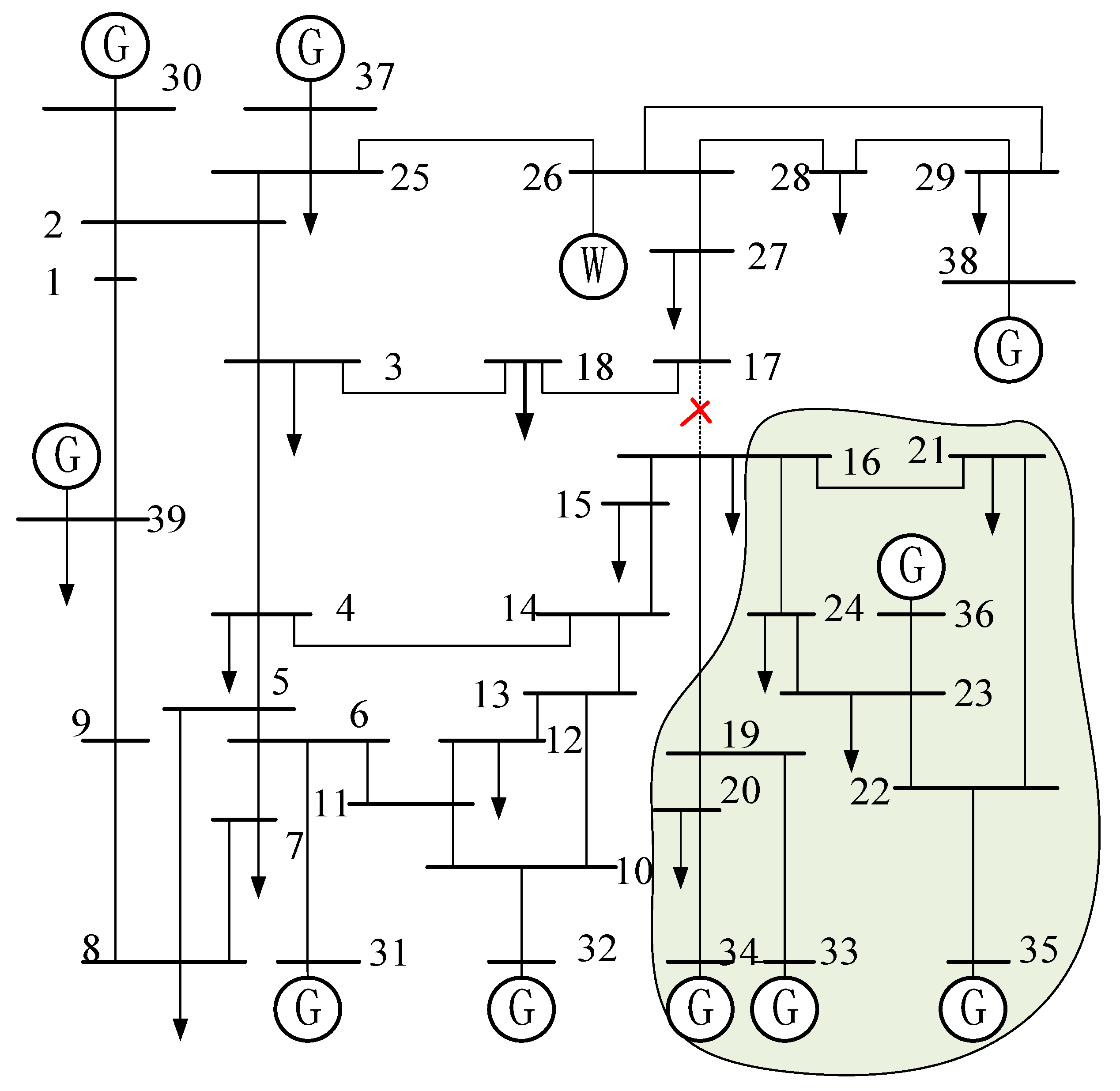
Therefore, this paper studies the optimal control of the closing angle of the subgrid parallel process in the power-system-recovery process. Based on considering the uncertainty of the wind-power output, the subgrid parallel process is realized, and the power loss load is restored to speed up the system-recovery process. Firstly, the uncertainty of wind-power output is described in the form of probability density prediction, and a probability-prediction model of wind-power output based on quantile regression LSTM is established. Based on predicting future wind-power output intervals, the probability density function of the output at each time point in the future is obtained through kernel density estimation, and various output probability scenarios of wind power are integrated through weight addition to improve the accuracy of wind-power prediction. The influence of wind-power output uncertainty on the closing angle and adjustment scheme is fully considered. Then, based on a consideration of the probability of wind-power output, a control model to reduce the phase angle difference at both ends of the parallel point is established by adjusting the active power output of the conventional units of the system and assigning as the control measure the load to be restored after power failure. In the regulation process, the multiobjective collaborative optimization is carried out with the minimum output adjustment sum of conventional units and the maximum input of important loads to be restored, and the NSGA-II algorithm is used to solve the established model. Finally, the effectiveness of the proposed method and model is verified by the IEEE 39-bus system simulation.

2. Prediction of Wind-Power probability Density Based on Quantile Regression LSTM

2.1. Quantile Regression Model

The principle of quantile regression is to split the data according to the dependent variable, form multiple quantiles, and study the regression relationship under multiple quantiles. In general, quantile regression has the following functions:

(1)

Analyze the influence trend of influencing factor X on variable Y.

(2)

Stability analysis for the regression model.

The assumed distribution function of the random variable is shown in Formula (1).

$$F(y)=\mathrm{Pr}(Y\le y)$$

(1)

The $\tau$ quantile of Y is defined as the minimum value $\tau$, satisfying $F(y)\ge \tau$, as shown in Formula (2).

$$Q(\tau )=\inf \{y:F(y)\ge \tau \};0<\tau <1$$

(2)

Assuming that a group of random samples of Y is $Y_1,Y_2,\dots Y_n$ and that this is affected by k influencing factors $X_1,X_1,\dots X_n$, the quantile regression of samples essentially minimizes the sum of absolute values of weighting errors, and the calculation formula is shown in Formula (3).

$$Q_Y(\tau |X)={\beta }_0(\tau )+{\beta }_1(\tau )X_1+\dots +{\beta }_k(\tau )X_k=\beta (\tau )X^{\prime }$$

(3)

where $Q_Y(\tau |X)$ represents the $X={[X_1,X_2,\dots ,X_k]}^T$ conditional quantile under the dependent variable y independent variable $\tau$; $\beta (\tau )=({\beta }_1(\tau ),{\beta }_2(\tau ),\dots ,{\beta }_k(\tau ){)}^T$ represents the regression coefficient vector at the $\tau$ quantile. Its expansion is shown in Formula (4).

$$\underset{\beta }{\min }{\displaystyle \sum _{i=1}^n{\rho }_{\tau }(Y_i-X_i^{\prime }\beta (\tau ))}$$

(4)

where ${\rho }_{\tau }(u)$ is the inspection function. The definition formula is shown in Formula (5).

$${\rho }_{\tau }(u)=(\tau -I(u<0))u$$

(5)

where $I(u)$ is an indicator function, $u$ is a conditional relationship, and when $u$ is true, $I(u)=1$, and vice versa: $I(u)=0$.

For the conditional quantile function, the parameter estimation value can be obtained by solving Formula (4), as shown in Formula (6).

$$\hat{\beta }=\arg {\min }_{\beta \in R}\left\{{\displaystyle \sum _{i=1}^n{\rho }_{\tau }(Y_i-X_i^{\prime }\beta (\tau ))}\right\}$$

(6)

In Formula (6), arg min represents the value of $\beta$ when the function takes the minimum value.

From the above analysis, for any $\tau \in (0,1)$, the parameter $\beta (\tau )$ is referred to as the $\tau$ regression quantile coefficient. The essence of quantile regression is to estimate different conditional quantiles of dependent variables by taking different $\tau$ values and using independent variables.

2.2. Network Model of Long- and Short-Term Memory

The traditional quantile regression model can effectively reflect the influence of independent variables on the distribution range and shape of dependent variables, but it is not suitable for nonlinear new energy output prediction. Taylor proposed a neural network quantile regression model (QRNN) by combining the nonlinear fitting of the neural network with the data analysis ability of QR. Based on the training mechanism of the original recurrent neural network (RNN), the network training results are more inclined to new information but show weak memory function. To solve the long-term dependence on RNN training, Hochreiter and Schmidhuber proposed the long-term and short-term memory network.

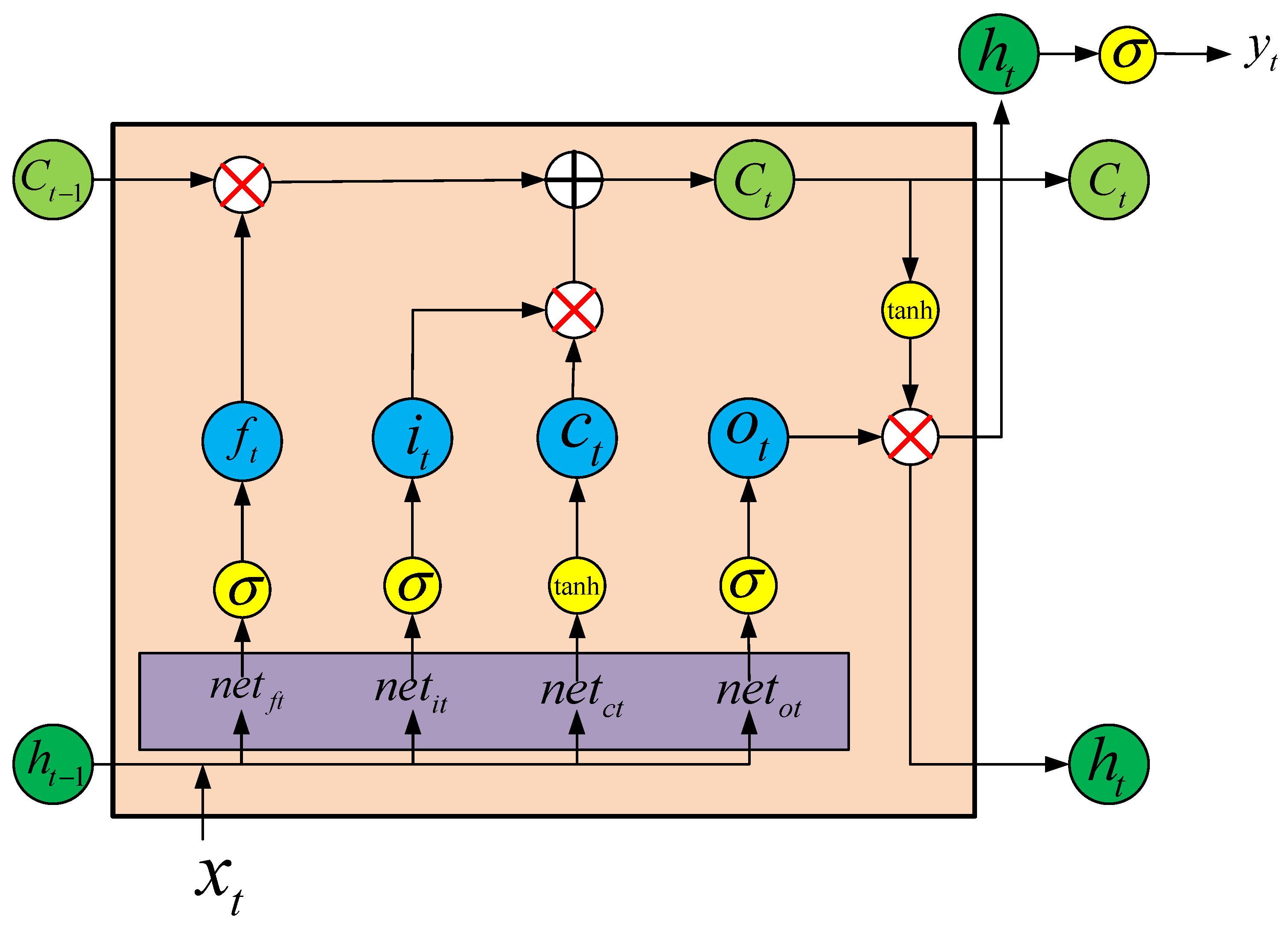
As a variant of the recurrent neural network, LSTM has a basic structure, as shown in Figure 1. LSTM is represented as a chain structure by time expansion, and the repetitive module of LSTM contains four neural network layers. The hidden layer in the RNN is replaced by a memory unit in the LSTM to realize effective memory of past information.

In the RNN network, the hidden layer has only one state, $h$, and a cell state, $c$, is added to the LSTM. Compared with the original RNN network, the LSTM is expanded according to the timeline, and the inputs are increased to three, including the cell state $c_{t-1}$ at the previous time, the output $h_{t-1}$ at the previous time, and the input $x_t$ at the current network. The outputs are increased to two, namely, the output $h_t$ of the LSTM at the current time and the cell state $c_t$ at the current time.

The LSTM has four gates in total. At each time, the LSTM receives the current time input $x_t$, the previously hidden state output $H_{t-1}$, and the memory cell state $C_{t-1}$ through three gates.

The first layer of neurons is the forgetting gate control layer, which helps LSTM decide to delete some information in the memory cell state, as shown in Formula (7).

$$f_t=\sigma (W_f[h_{t-1},x_t]+b_f)$$

(7)

The second layer and the third layers are the input gate and tanh layer, respectively, as shown in Formulas (8) and (9). Using the input gate, $i_t$, to determine the new information, $C_t^{\prime }$, to be stored in the new cell state, the tanh layer creates a new candidate value—$C_t^{\prime }$.

$$i_t=\sigma (W_i[h_{t-1},x_i]+b_i)$$

(8)

$$C_t=\tan h(W_C[h_{t-1},x_t]+b_C)$$

(9)

$$C_t^{\prime }=f_t^{*}{C}_{t-1}+i_t^{*}{C}_t$$

(10)

where $f_t^{*}{C}_{t-1}$ determines how much information is forgotten $C_{t-1}$; $i_t^{*}{C}_t$ determines how much information is stored in the new cell state $C_t$.

Finally, calculate $\sigma$ through the output gate, $H_t$. As shown in Formula (11), after Formula (10) passes through the tanh layer, it is multiplied by the output gate to bring the forgetting and memory parameters to the final output.

$$O_t=\sigma (W_o[h_{t-1},x_t]+b_o)$$

(11)

$$h_t=O_t\tan h(C_t)$$

(12)

where $W_f, b_f, W_i{b}_i$ are the weight and offset of the forgetting gate and the input gate, respectively; $W_C, b_C, W_O, b_O$ are the updated value and the weight and offset of the output gate, respectively; $\sigma (\cdot )$ is an activation function; $\tanh (\cdot )$ is a tangent activation function. Reference numeral $[h_{t-1},x_t]$ denotes a combination of matrices having the same number of rows.

As a deep neural network with memory ability, LSTM has been widely used in nonlinear sequence prediction. Compared with a static neural network, LSTM can better explore the correlation between sequence data and is very suitable for dealing with problems highly related to time series [7,8].

2.3. Nuclear Density Estimation

As one of the nonparametric estimation methods, kernel density estimation is often used to estimate the unknown density function in probability theory. Nonparametric estimation does not need to assume the distribution function of the sample data in advance. It can directly analyze the sample data, study the data analysis characteristics, simulate the real probability density curve, and realize the estimation of the sample data.

Assuming that there are $k$ random discrete samples $X_1,X_2,\dots ,X_k,$ and the probability density function is $f(x)$, the kernel density estimation formula of the probability density function is shown in Formula (13).

$${\hat{f}}_h(x)=\frac{1}{kh}{\displaystyle \sum _{i=1}^{k}K(\frac{x-X_i}{h})}=\frac{1}{h}{\displaystyle \sum _{i=1}^k{K}_h}(x-X_i)$$

(13)

where $h$ is the bandwidth; $k$ is the sample volume; $x$ is a one-dimensional array with equal spacing; $X_i$ is the $i$ data in the time series sample, $i=1,2,\dots ,k$; $K(y)$ is a kernel function. Generally, Gauss, matrix, triangle, etc., can be selected. In this paper, the Gaussian kernel function (GKF) is selected, and the expression is shown in Formula (14).

$${\hat{f}}_h(x)=\frac{1}{kh}{\displaystyle \sum _{i=1}^{k}K(\frac{x-X_i}{h})}=\frac{1}{h}{\displaystyle \sum _{i=1}^k{K}_h}(x-X_i)$$

(14)

where $\eta$ is the smoothing parameter of bandwidth, $\eta >0$, and its height affects the shape of the distribution. The optimal bandwidth can be determined by the plug-in bandwidth selector. In this paper, the empirical rule is used to select the appropriate bandwidth, and the expression is shown in Formula (15).

$$h\approx 1.06\hat{\sigma }{k}^{-\frac{1}{5}}$$

(15)

In Formula (15), $\hat{\sigma }$ is the estimated standard deviation; $k$ is the number of samples.

2.4. Wind-Power Probability Density Prediction Process Based on Quantile Regression LSTM

(1) Normalize the obtained historical wind power data, as shown in Formula (16), to reduce the training time and improve the accuracy of the model.

$$X_t=\frac{X_t-X_{\min }}{X_{\max }-X_{\min }}$$

(16)

where $X_t$ is the sample data at a time $t$, and $X_{\max },X_{\min }$ are the maximum value and minimum value of all samples, respectively.

(2) Divide the training set and the test set, determine the parameters of each layer in the LSTM network, and preset the required number of loci.

(3) The test set is input into the trained LSTM model for power prediction, and the power prediction results under each quantile are obtained.

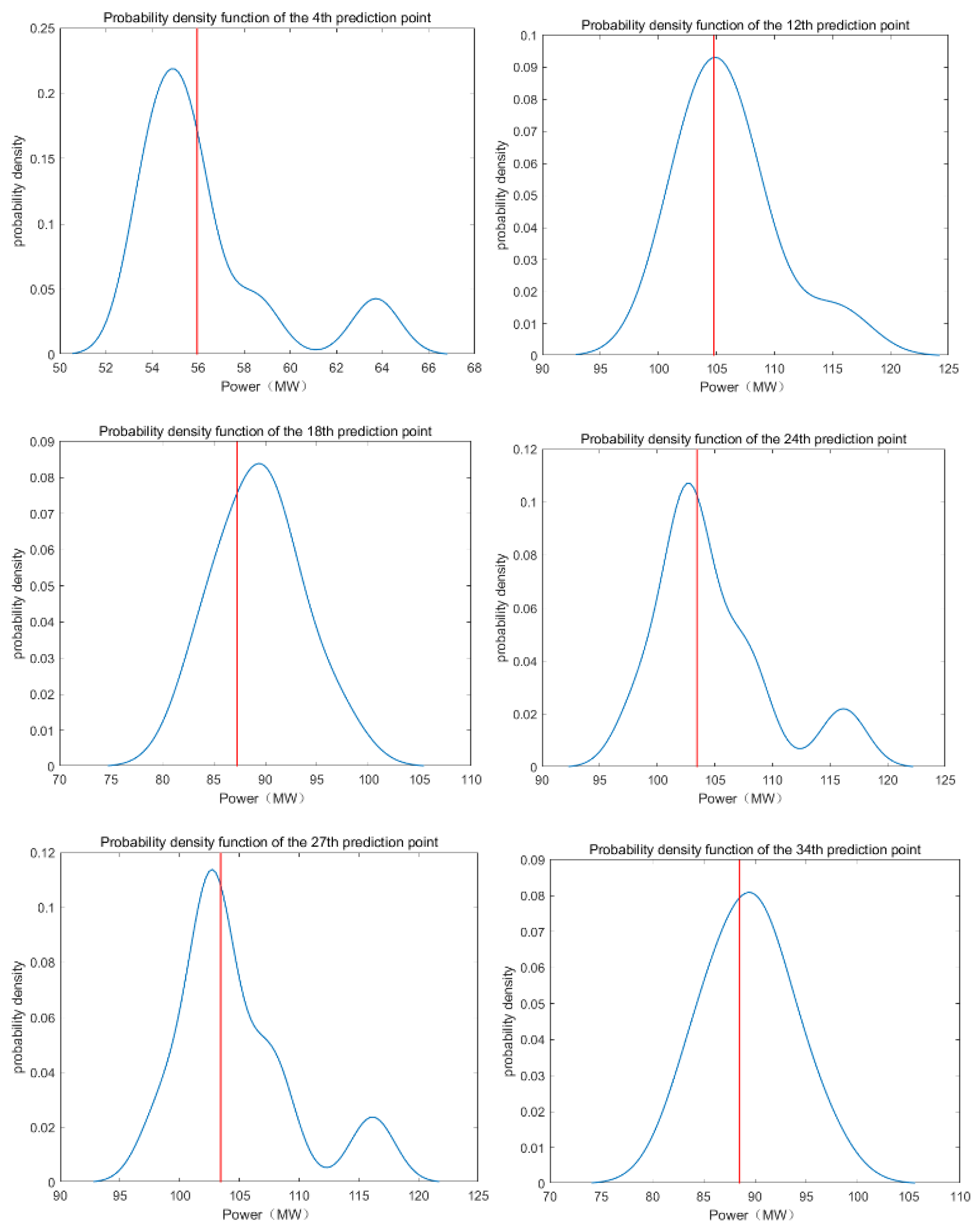
(4) The kernel density estimation is performed on the prediction results at each quantile obtained by training, and the probability density function at each prediction point is calculated.

The specific prediction process is shown in Figure 2.

2.5. Model Evaluation Index

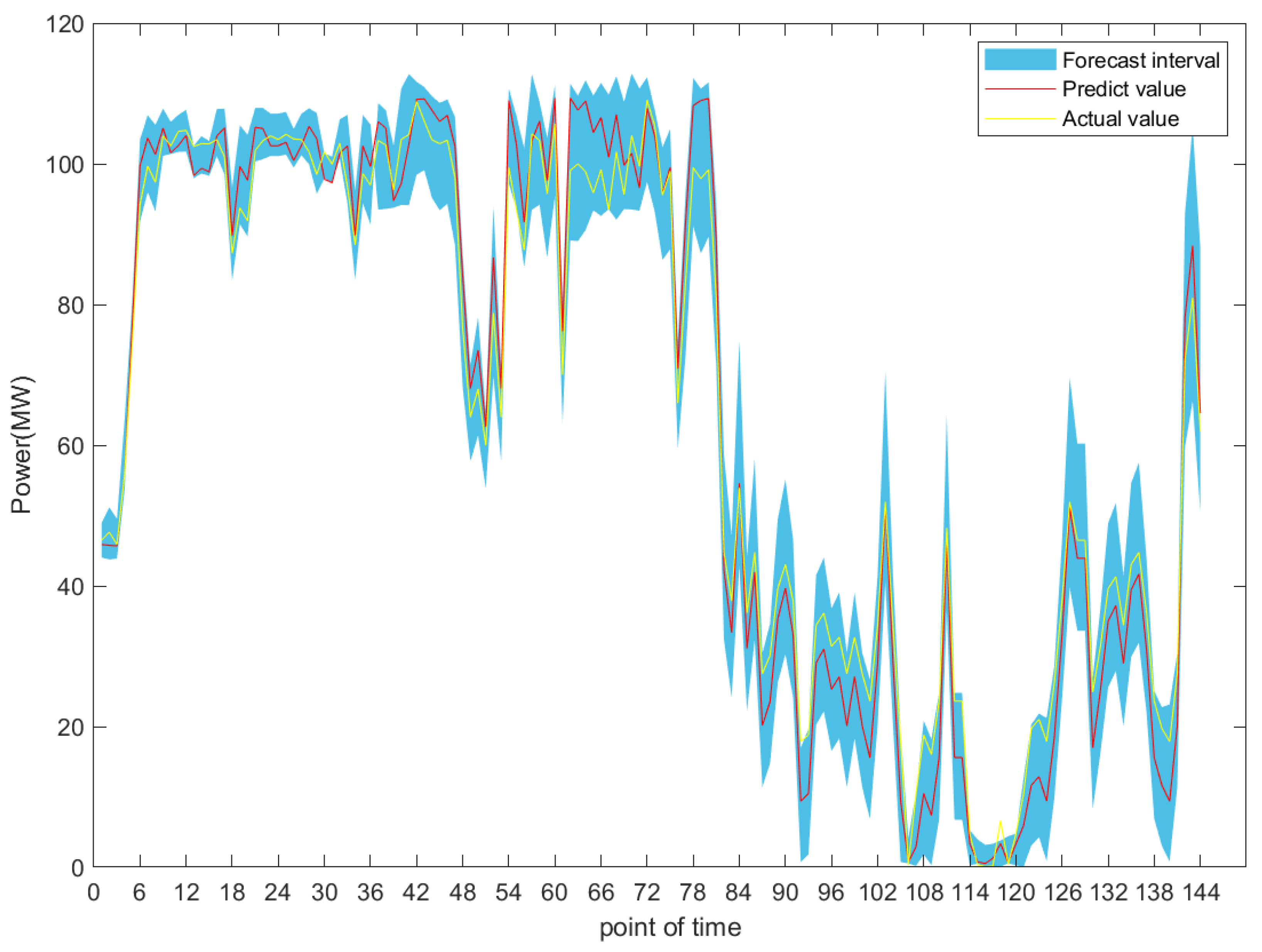
After the wind-power interval-prediction results are obtained, the following two indicators are used to evaluate the accuracy of the model prediction.

(1) Interval coverage (reliability):

The larger the coverage of the interval, the higher the reliability of the model.

$$PICP=\frac{1}{N}\xi \ast 100\%$$

(17)

where $PICP$ is the interval coverage rate and $\xi$ is the number of actual values falling within the interval.

(2) Interval average width (sensitivity):

When the prediction interval is large enough, the reliability of the prediction can be improved. However, at this time, wind power cannot be effectively predicted and has no practical value. Therefore, the average interval width is used to evaluate the prediction interval width to ensure the validity of the prediction.

$$PINAW=\frac{1}{N}{\displaystyle \sum _{i=1}^N(U_i-L_i)}$$

(18)

where $PINAW$ is the average interval width, $U_i$ is the upper limit value of the $i$ prediction interval, and $L_i$ is the lower limit value of the $i$ prediction interval.

2.6. Summary

LSTM has a good fitting ability for nonlinear time series and has a good prediction effect in medical protein structure prediction, road traffic flow rate prediction, etc. Probability density is mainly used to obtain the probability density curve, provide the fluctuation range of wind power, and obtain more useful information. Quantile regression is used to combine the two, and regression prediction is conducted under different quantiles. Finally, nuclear density estimation is used to calculate the probability density function, which provides wind power information for the subsequent optimal regulation model of closing angle.

3. Optimal-Control Model of the Parallel Closing Angle of Ring Network Considering Wind-Power Uncertainty

Compared with the radiative grid structure with poor resistance to source and load fluctuations, the ring network can not only improve network security and enhance system transmission capacity but can also withstand the power fluctuations of new energy and better support the recovery of important loads. Through the analysis of the power grid structure and the trend of power flow, the voltage phase angle of the nodes at both ends of the line to be paralleled is studied. Generally, the power grid is divided into the sending end and the receiving end according to the voltage phase angle of the nodes at both ends. By reducing the active power from the sending end to the receiving end, the phase angle difference of the node voltages at both ends can be effectively reduced. Generally, the phase angle difference at both ends is reduced by inputting the load at the sending end and increasing the output of the unit at the receiving end.

Due to the uncertainty of wind-power output, the fluctuation of active power output after grid connection will cause the power flow fluctuation of the access point, thus causing the phase angle fluctuation of the point to be paralleled. Through the probability density prediction of wind-power output, this paper not only further improves the prediction accuracy, but also integrates various output probability scenarios of wind power, and fully considers the impact of the uncertainty of wind-power output on the closing angle and the adjustment scheme.

Based on considering the uncertainty of new energy output, this paper establishes a control model to reduce the phase angle difference at both ends of the parallel point by adjusting the active output of the conventional unit of the system and putting the load to be restored after power failure as the control measure. In the process of regulation and control, multiobjective collaborative optimization is carried out considering that the sum of output adjustment of conventional units is the smallest and the most important loads to be restored are input.

3.1. Objective Function

(1) Minimum sum of the regulated output of the conventional unit

During system recovery, to speed up the system-recovery process and reduce the regulation cost, the minimum output adjustment sum of conventional units in the regulation process is taken as the objective function I, which is defined as:

$$\min f_1={\displaystyle \sum _{s=1}^k{P}_s}\ast [{\displaystyle \sum _{i=1}^n(P_{Gis}-P_{Gi0})}]$$

(19)

where $P_s$ is the probability value of different output scenarios of wind power; $P_{Gis}$ is the adjustment value of generator output considering different wind-power output probabilities; $P_{Gi0}$ is the initial output value of the conventional unit; $n$ is the number of generator nodes.

(2) Maximum weight of the load to be restored

In the process of system restoration, the load with high importance shall be preferentially restored to minimize the outage loss. Therefore, objective function II is to maximize the total load restoration weight in the regulation process, which is defined as:

$$\max f_2={\displaystyle \sum _{s=1}^k{P}_s}\ast \left({\displaystyle \sum _{i=1}^N{\displaystyle \sum _{l=1}^m{c}_{ils}{\omega }_{il}{P}_{Lil}}}\right)$$

(20)

where $c_{ils}$ represents whether the feeder $l$ connected to the node $i$ is restored. If it is restored, the value is 1—otherwise, it is 0; ${\omega }_{il}$ is the load weight of the feeder $l$ connected to the node $i$; $P_{Lil}$ is the load value of the feeder $l$ connected to the node $i$; $N$ is the total number of system nodes; $m$ is the number of feeders connected to a node $i$.

Based on the objective function of the minimum sum of the regulated output of conventional units and a maximum weight of the load to be restored, the general objective of optimal control of the parallel closing angle of the ring network is defined as follows:

$$\min F=[f_1,-f_2]$$

(21)

3.2. Constraint Condition

The constraints included in the model are as follows:

$$P_{Gi}+P_{wis}-{\displaystyle \sum _{l=1}^m{c}_{ils}}{P}_{Lil}-P_{dresi}={\displaystyle \sum _{i,j}{P}_{ij}},i=1,2,\dots ,N$$

(22)

$$Q_{Gi}+Q_{wis}-{\displaystyle \sum _{l=1}^m{c}_{ils}}{Q}_{Lli}-Q_{dresi}={\displaystyle \sum _{i,j}{Q}_{ij}},i=1,2,\dots ,N$$

(23)

$$P_{ij}={U_i}^2{G}_{ij}-U_i{U}_j(G_{ij}\cos {\theta }_{ij}+B_{ij}\sin {\theta }_{ij})$$

(24)

$$Q_{ij}=-U_i^2(B_{ij}+B_{ij}^C)-U_i{U}_j(G_{ij}\sin {\theta }_{ij}-B_{ij}\cos {\theta }_{ij})$$

(25)

$$P_{gi0}\le P_{gi}\le P_{gi}^{\max }$$

(26)

$$Q_{gi0}\le Q_{gi}\le Q_{gi}^{\max }$$

(27)

$$U_i^{\min }\le U_i\le U_i^{\max }$$

(28)

$$\left|P_{ij}\right|\le P_{ij}^{\max }$$

(29)

$$\left|{\theta }_{mn}\right|\le {\theta }_{set}$$

(30)

$$\Delta f(c_{il}{P}_{Lil})\le \Delta f_{\max }$$

(31)

Formulas (22)–(31) are the constraint conditions to be met in the process of closing angle regulation. Equations (22) and (23) are constraints of active power balance and reactive power balance of nodes, where $P_{dresi}$, $Q_{dresi}$ are the restored loads of node $i$; $P_{wis}$, $Q_{wis}$ are the active output and reactive output of the wind farm, respectively, connected to node $i$ under different probabilities, $P_s$; $P_{Gi}$, $Q_{Gi}$ are the active output and reactive output of the conventional unit connected to node $i$, respectively. Equations (24) and (25) are the active and reactive power calculation formulas of the line $(i,j)$ flowing through the $i$ end, where $U_i$,$U_j$ is the voltage of the node $i$, $j$; $G_{ij}$, $B_{ij}$ and ${\theta }_{ij}$ are the conductance and susceptance of the line $(i,j)$ and the phase angle difference of the nodes at both ends of the line, respectively; $B_{ij}^C$ is the susceptance parameter of the $i$ end to the ground branch of the $\Pi$ type equivalent circuit of the line $(i,j)$. Equations (26)–(29) are inequality constraints for safe operation of the power system, which are unit active output constraints, unit reactive output constraints, node voltage constraints, and tie line transmission power constraints; here, $P_{gi0}$ and $Q_{gi0}$ are the initial active output and reactive output of conventional units, respectively. During system recovery, the system has a large power loss load, and most units are in an upward-climbing state. To accelerate the recovery process, It is required that all units are not allowed to operate with reduced output; $P_{gi}^{\max }$ and $Q_{gi}^{\max }$ are the maximum active output and reactive output allowed for unit operation, respectively; $U_i^{\min }$ and $U_i^{\max }$ are the allowable lower and upper limits of the node voltage, respectively; $P_{ij}^{\max }$ is the maximum power allowed to flow through the line $(i,j)$. Equation (30) is the phase angle difference constraint at both ends of the line to be paralleled and ${\theta }_{set}$ is the maximum setting value allowed in system recovery. Equation (31) is the constraint of system frequency change caused by load input and $\Delta f_{\max }$ is the maximum frequency drop value caused.

3.3. Model Solving

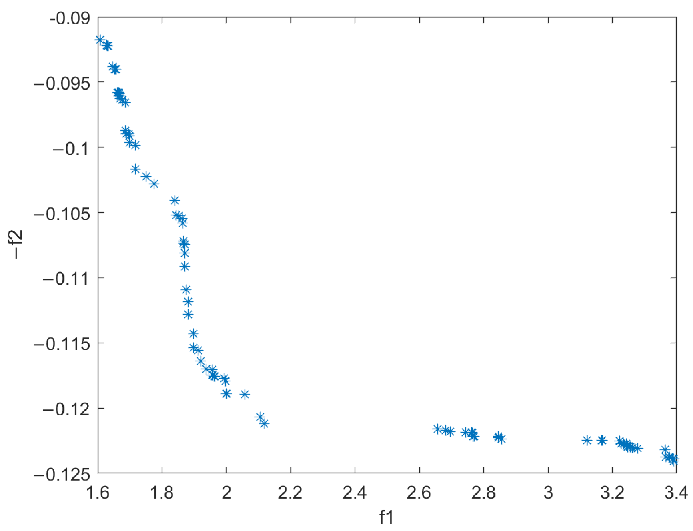
The optimal-control model of the parallel closing angle of the power system loop network considering the uncertainty of wind-power output established in this paper is a multiobjective nonlinear programming problem, and its standard form is:

$$\{\begin{array}{l}\min F(x)=[f_1(x),-f_2(x)]\\ s.t.\{\begin{array}{l}{g}_i\left(x\right)=0\hspace{1em}i=1,2,\dots ,n\\ h_k\left(x\right)\le 0\hspace{1em}k=1,2,\dots ,m\end{array}\end{array}$$

(32)

where $f_1(x)$ and $f_2(x)$ are the two objective functions of minimum unit output adjustment and maximum load weighted recovery, respectively; $x$ is an $n$-dimensional decision variable, including the output value of the conventional unit after adjustment, determining whether the feeder connected to each bus is restored; $g_i\left(x\right)$ is an equality constraint function; $h_k\left(x\right)$ 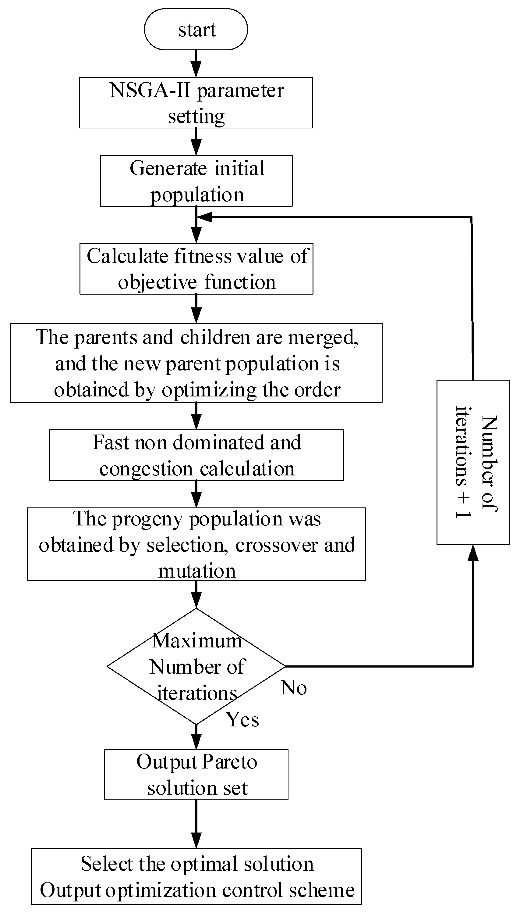is an inequality constraint function. This paper uses the NSGA-II algorithm to solve the established model, and the specific solution process is shown in Figure 3. Finally, the fuzzy multi-attribute decision-making scheme is used to select the optimal solution in the Pareto solution set. The formula is as follows.

$${\mu }_j^k=\frac{f_j^{\max }-f_j^k}{f_j^{\max }-f_j^{\min }}$$

(33)

$${\mu }^k=\frac{{\displaystyle \sum _{j=1}^{\mathrm{n}}{\mu }_j^k}}{{\displaystyle \sum _{k=1}^{\mathrm{m}}{\displaystyle \sum _{j=1}^{\mathrm{n}}{\mu }_j^k}}}$$

(34)

$$opt=\left\{o|{\mu }^o=\max ({\mu }^k)\right\}$$

(35)

Use Equation (33) to standardize the data and use Equation (34) to calculate the proportion of the sum of the attributes of each solution in the population. Finally, use Equation (35) to select the solution with the largest proportion of the population as the optimal solution.

Compared with the multiobjective genetic algorithm using non-dominated sorting and sharing, NSGA-II proposed a non-dominated sorting genetic algorithm with an elite strategy, reducing the computational complexity of the algorithm from $O(M{N}^3)$ to $O(M{N}^2)$, where M is the number of objective functions and N is the population size. NSGA-II has good performance in solving problems with less than three objective dimensions.

4. Case Analysis

4.1. Case Analysis of Wind-Power Probability Density Prediction

The historical measured data of a wind farm in China in July 2017 is selected as the sample for short-term wind-power probability density prediction. The rated capacity of the wind farm is 150 MW, the data sampling interval is 10 min, and a total of 4464 pieces of data are used, as shown in Figure 4.

The dataset is divided. The data of the previous 30 days comprise the training set, and the data of the 31st day comprise the test set, with an interval of 10 min at each time point. An LSTM network with three hidden layers is built through the Keras deep learning framework. The number of neurons in the hidden layer is 32. The optimization algorithm uses adaptive time estimation (Adam). The maximum number of iterations for the LSTM network under each quantile is set to be 100, the initial learning rate is 0.005, the penalty parameter is 1, the kernel function of the quantile regression parameter is Gaussian function, the quantile is $\tau \in (0,1)$, and the interval is 0.1. The training process of the LSTM network is shown in Figure 5 (taking $\tau =0.5$ as an example).

According to Figure 5, after 60 training rounds are completed, the root mean square error (RMSE Blue data in the figure) and loss values of the mean square error (MSE Orange data in the figure) tend to be stable. According to the above modeling conditions, run the established model to obtain the wind-power output prediction results of the test set data under the 90% confidence interval, as shown in Figure 6.

As shown in Figure 6, when the wind power fluctuates greatly, the model can also show good fitting ability. The evaluation index is used to evaluate the model prediction results. The interval coverage rate of the model prediction is 91.67%, and the average interval width is 22.64. Most of the actual values can fall within the confidence interval, which can meet the prediction requirements.

The probability density function curves at different time points in the prediction period are obtained by kernel density estimation. The probability density function curves at 6 time points of 4, 12, 18, 24, 27, and 34; these are randomly selected, as shown in Figure 7.

As shown in Figure 7, from the predicted probability density function, the real values fall on both sides near the middle of the density function, which can better explain the probability density of wind-power output at the predicted time point in the future.

To further cope with the uncertainty of wind-power output, the wind-power output interval at the prediction time is reasonably divided. As shown in Figure 8, taking the probability density function of the 25th prediction point as an example, the average value in the interval is taken as the output value of wind power, and the area of each interval in the total area of the selected area is taken as the probability of the output scenario, forming multiple scenarios of wind-power output at that time. See

Table 2. Wind-power output value and corresponding probability.

Wind Power (MW)	Probability
96	0.1
99	0.2
103	0.52
107	0.08
116	0.1

for specific values.

4.2. Case Analysis of Closing Angle Regulation Scheme Based on Probability Density Prediction

Taking the New England 10-machine 39-bus system as an example, this paper analyzes the closing angle regulation example to verify the effectiveness of the proposed model. The model is established in matlabr2019a, and the model is solved by the NSGA-II algorithm. The simulation computer condition is inter-core i5 and the memory is 8 GB.

As shown in Figure 9, the 39 nodes of New England’s 10 machines are assumed to be disconnected from the lower-right subnetwork after a power outage caused by a failure of the lower-right subnetwork. After a power outage, the main network transmits power to the subnetwork through lines 15–16 to realize the black start of the subnetwork. To realize the stable operation of the subnetwork, reduce the risk of subnetwork load recovery, and reduce the transmission power of lines 15–16. The next step is to restore lines 16–17 and perform the parallel operation of the ring network. To share the power flow of heavy load lines 15–16, strengthen the connection between the main network and the subnetwork, and improve the operation stability of the whole system. To ensure the smooth operation of parallel operation, the phase angle difference at both ends of lines 16–17 to be parallel shall be limited within the maximum allowable value. When the wind-power output is the predicted value of 100 MW, the phase angle difference at both ends of the line is 23.32°. ${\theta }_{set}=$20° is set to ensure the safety of the closing process. The operating parameters of the generator and the recovered load data under the initial operating state are shown in

Table 3. Initial operating parameters of the generator.

Node	${\mathit{U}}_{\mathit{G}\mathit{i}0}$	${\mathit{P}}_{\mathit{G}\mathit{i}0}$	${{\mathit{P}}_{\mathit{G}\mathit{i}}}^{\mathbf{max}}$	${{\mathit{Q}}_{\mathit{G}\mathit{i}}}^{\mathbf{min}}$	${{\mathit{Q}}_{\mathit{G}\mathit{i}}}^{\mathbf{max}}$
30	1.048	3.4	3.5	−2.8	3.15
31	0.982	3.45	11.46	−9.17	10.3
32	0.983	3.5	7.5	−6	6.75
33	0.997	4.5	7.32	−5.86	6.59
34	1.012	6	6.08	−4.86	5.47
35	1.049	4	7.5	−6	6.75
36	1.064	5.6	6.6	−5.28	5.94
37	1.028	4.6	6.4	−5.12	5.76
38	1.027	3.8	7.6	−7.44	8.37
39	1.03	8	11	−8.8	9.9

and

Table 4. Initial operating load data.

Node	${\mathit{P}}_{\mathit{d}\mathit{r}\mathit{e}\mathit{s}\mathit{i}}$	${\mathit{Q}}_{\mathit{d}\mathit{r}\mathit{e}\mathit{s}\mathit{i}}$	Node	${\mathit{P}}_{\mathit{d}\mathit{r}\mathit{e}\mathit{s}\mathit{i}}$	${\mathit{Q}}_{\mathit{d}\mathit{r}\mathit{e}\mathit{s}\mathit{i}}$
1	2.52	1.19	20	2.80	1.03
3	3.22	0.03	21	2.24	1.15
4	5.00	1.84	23	1.98	0.85
7	2.34	0.84	24	2.09	−0.92
8	2.22	1.76	25	2.24	0.47
9	1.04	1.25	26	2.39	0.17
12	0.09	0.90	27	2.81	0.76
15	3.20	1.53	28	3.06	0.28
16	2.79	0.33	29	2.04	0.27
18	3.08	0.30

(both are standard unit values). Node 26 is connected to the wind farm, with an installed capacity of 150 MW, and the output probability is shown in Table 2. At nodes 8, 16, 20, 21, 23, and 24, there are 20, 10, 20, 10, 10, and 10 feeders, respectively, whose loads are to be restored. The load and weight on each feeder are generated randomly and the power factor is consistent. The upper- and lower-unit values of the node voltage are 1.1 and 0.95, respectively. The NSGA-II parameters are set as follows: the population size is 120, the crossover probability is 0.9, the mutation probability is 0.1, and the maximum number of iterations is 150.

The optimal regulation model of closing angle is solved based on NSGA-II, and the cumulative time is 187 s. The obtained multiobjective Pareto solution is shown in Figure 10.

The fuzzy multi-attribute decision-making method mentioned above is used to select the optimal solution from the Pareto set. The calculation results of the decision index values under each scheme are shown in Figure 11.

According to Figure 11, the decision index value of scheme 57 is the largest, so it is the optimal solution, and the corresponding objective function values are $f_1=$ 2.06 and 0.1189. The corresponding unit output adjustment is shown in

Table 5. Adjustment of generator active output.

Node	$\mathbf{\Delta }{\mathit{P}}_{\mathit{G}\mathit{i}}$
31	0.55
37	1.02
38	0.49

, and the restored load outgoing line and load are shown in

Table 6. Feeder load recovery.

Node	Feeder	Weight	Load	Node	Feeder	Weight	Load
8	1	0.418	0.042	20	16	0.448	0.017
	2	0.62	0.067		17	0.719	0.025
	3	0.837	0.039		19	0.679	0.016
	7	0.608	0.056		20	0.746	0.067
	13	0.646	0.056	21	1	0.951	0.05
	15	0.752	0.016		2	0.526	0.035
	16	0.75	0.026		9	0.963	0.064
	17	0.47	0.052	23	1	0.922	0.085
	18	0.545	0.065		3	0.994	0.013
16	2	0.65	0.05		5	0.523	0.096
	3	0.523	0.073		6	0.832	0.052
	4	0.661	0.049		7	0.998	0.036
	5	0.832	0.097		8	0.715	0.075
	6	0.661	0.047		10	0.666	0.031
	9	0.921	0.033	24	2	0.748	0.078
20	1	0.699	0.081		5	0.663	0.062
	11	0.697	0.065		6	0.871	0.039
	12	0.823	0.038		7	0.795	0.086
	15	0.509	0.059

.

Table 5 only shows the units which exhibit a change in output. It can be seen from the table that three units are participating in the output adjustment in the regulation, namely units 31, 37, and 38—the adjustment amounts for these are 0.55, 1.02, and 0.49, respectively, and the accumulated output increase is 206 MW. According to the operating parameters of the generator, the generator units involved in the adjustment still have a large adjustable capacity, which indicates that the regulatory scheme in this paper has a strong ability to regulate the closing angle and can also achieve effective regulation of the closing angle in the case of insufficient standby capacity of the system.

According to Table 6, the total restored load of this regulation scheme is 193.6 MW, of which the total number of feeders restored at nodes 8, 16, 20, 21, 23, and 24 is 9, 6, 8, 3, 7, and 4, respectively. According to the weight of the restored feeder load, the restoration scheme formulated by the model established in this paper can give priority to the restoration of more important loads while the total restored load is the largest, which is helpful to improve the load recovery efficiency and reduce the outage loss.

The power flow results of lines 15–16 before and after regulation are shown in

Table 7. Branch current of lines 15–16.

	P (MW)	Q (Mvar)
Before regulation	800.76	175.42
After regulation	650.63	158.65

(at this time, the wind-power output is 100 MW).

According to the data in Table 7, the transmission active power of the system interconnection line 15–16 is as high as 800.76 MW before the regulation, which is close to the power limit of the interconnection line. After the regulation of the system generator output and feeder load, the transmission active power of lines 15–16 is reduced to 650.63 MW, which effectively alleviates the heavy load problem of lines 15–16 and is conducive to improving the stability of the system parallel process.

The voltage results at both ends of the corresponding line to be closed under different wind-power output scenarios are shown in

Table 8. Voltage values of nodes 16 and 17 under different wind-power output scenarios.

Wind Power (MW)	Node 16		Node 17		Phase Angle Change Value (°)
	Amplitude (pu)	Phase Angle (°)	Amplitude (pu)	Phase Angle (°)
50	1.022	5.118	1.004	−13.454	18.572
96	1.023	6.025	1.005	−11.721	17.746
99	1.023	6.084	1.005	−11.609	17.693
103	1.023	6.163	1.005	−11.459	17.622
107	1.023	6.241	1.005	−11.309	17.55
116	1.023	6.417	1.005	−10.973	17.39
150	1.023	7.081	1.006	−9.706	16.787

.

According to the data in Table 8, in the division of wind-power output probability scenarios, the closing angle limit under each scenario does not exceed 20°. To further consider the extremes of wind-power output, when the wind-power output is not within the predicted range and there is a large fluctuation, Table 8 gives the node voltage results when the wind-power output is 50 MW and 150 MW, respectively. The data show that the phase angle difference between the nodes at both ends is still within the set range and does not exceed the limit, the proposed regulatory scheme can better deal with the closing angle fluctuation caused by the uncertainty of wind-power output.

4.3. Analysis of the Regulation Scheme of Closing Angle under Deterministic Conditions

To further explain the impact of the uncertainty of wind-power output on the closing angle of the system, the wind-power output is taken as a fixed value, and a deterministic optimal regulation scheme is given. The generator output under the deterministic regulation scheme is shown in

Table 9. Generator adjustment when wind-power output is fixed.

Node	$\mathbf{\Delta }{\mathit{P}}_{\mathit{G}\mathit{i}}$
37	0.99
38	0.4

. The load recovery is shown in

Table 10. Load recovery when the wind-power output is constant.

Node	Feeder	Load
8	1/2/3/5/7/8/17/18	0.44
16	5/9	0.13
20	4/11/12/15/16/17/19	0.253
21	1/6/9	0.132
23	1/3/6/7/10	0.216
24	8/10	0.072

.

According to the data in Table 9 and Table 10, the total amount of generator output adjustment involved in the regulatory scheme under the wind-power output determination is 139 MW, which is 58 MW less than the optimal regulation scheme for the closing angle under wind-power output uncertainty. The number of load feeders recovered is 27, and the total amount of recovery is 124.4 MW. Compared with the uncertain regulation scheme, the total adjustment number of generators is reduced by 10 and 69.2 MW, respectively. Although the total adjustment number of generators is reduced, the total load recovery amount is also reduced. In addition, when the wind-power output fluctuates, the adopted regulation scheme may be difficult to ensure that the closing angle is within the controllable range. Figure 12 shows the closing angle values under different wind-power output scenarios under the implementation of the deterministic optimization scheme.

It can be seen from Figure 12 that, when the optimization scheme is adopted to determine the wind-power output, the phase angle difference between the two points to be paralleled may exceed the limit. In this paper, the wind power access node belongs to the receiving end system, and the closing angle will increase due to the reduction in the wind-power output. At this time, if the definite optimization scheme is adopted, it will be difficult to ensure that the closing angle is controlled within the allowable range; this proves the applicability of the scheme proposed in this paper under the consideration of the uncertainty of wind-power output. In other words, when the wind-power output fluctuates significantly, the closing angle is still within the allowable range and does not exceed the limit.

4.4. Summary

In the actual operation process, since the system is in a dynamic adjustment process and the closing angle is in a state of change due to the influence of various uncertain factors in the system, the actual operator can make full use of the real-time information provided by the wide-area measurement system. This is the case on both sides of the line which is to be connected to the grid to monitor the phase angle, voltage difference, frequency, and other data at both ends in real time. This also issues the closing command after meeting the grid connection conditions.

From the above analysis, the regulation scheme obtained by the model established in this paper can better solve the closing-angle out-of-limit problem caused by the uncertainty of the electric output in the parallel operation of power systems. Through the solution of the objective function, the obtained regulation scheme can ensure the recovery of the most important load and reduce the heavy load, while minimizing the total output adjustment of the conventional units; this plays a positive role in improving the stability of the system.

5. Conclusions

This paper studies the closing-phase angle control when the subnetworks are parallel in the recovery process of the power system after wind power and other new energies are connected. The wind-power output prediction is modeled using probability density prediction, and the wind-power output is described in the form of output probability. This forms multiobjective optimal regulation model to restore the most important loads of the outage feeders. Through theoretical analysis and numerical simulation analysis, the following conclusions can be drawn:

(1) Compared with traditional deterministic prediction, the quantile regression LSTM model established in this paper can effectively quantify the uncertainty of wind-power output by predicting the probability density of wind power in the future; furthermore, it can provide data support for the supply–demand balance and safe and stable operation of the power system.

(2) Compared with robust optimization, this paper obtains the probability distribution of wind-power output and using probability weighting. Taking a scenario under the maximum output probability of wind power into consideration, it also satisfies a scenario when the wind-power output is at both ends of the interval. This consideration ensures robustness and reduces conservatism to a certain extent.

(3) The established multiobjective optimal regulation model can achieve the minimum output adjustment of conventional units and the maximum recovery of important loads in the process of satisfying the regulation of the closing angle. The multiobjective solution is adopted to ensure the advantages and disadvantages of understanding, effectively accelerate the process of system recovery, and reduce the loss of power outage.

The here-presented method for controlling closing angles is necessary when a system is still in the process of recovery, its grid structure is preliminarily formed, and its operation is not yet stable. Therefore, this paper does not consider the impact of the dynamic thermal rating (DTR) of overhead lines on their transmission power [45,46]. The application of dynamic transmission capacity assessment technology for overhead lines will change the maximum transmission capacity of lines, which is conducive to improving the transmission capacity of a system [47]. When a system recovers to a stable operation state, the current-carrying capacity of overhead lines can be evaluated based on the heat balance equation; the dynamic capacity of a line is embedded into the power flow constraint of the optimization model. This is conducive to further improving the stability of the closing process. Optimization models which consider the closing angle regulation of DTR require further study.

References

1. Xu, X.; Wang, H.; Yan, Z.; Lu, Z.; Kang, C.; Xie, K. Overview of power system uncertainty and response methods in the context of energy transformation. Power Syst. Autom. 2021, 45, 2–13. [Google Scholar]
2. Wan, C.; Song, Y. Probability prediction theory and method of new energy power system and its application. Power Syst. Autom. 2021, 45, 2–16. [Google Scholar]
3. Li, T.; Wang, Y.; Zhang, N. Combining Probability Density Forecasts for Power Electrical Loads. IEEE Trans. Smart Grid 2020, 11. [Google Scholar] [CrossRef]
4. He, Y.; Liu, R.; Li, H.; Wang, S.; Lu, X. Short-term power load probability density forecasting method using kernel-based support vector quantile regression and Copula theory. Appl. Energy 2017, 185, 254–266. [Google Scholar] [CrossRef]
5. Zhou, Y.; Cui, Z.; Lin, K.; Sheng, S.; Chen, H.; Guo, S.; Xu, C.-Y. Short-term flood probability density forecasting using a conceptual hydrological model with machine learning techniques. J. Hydrol. 2021, 604, 127255. [Google Scholar] [CrossRef]
6. Yang, Y.; Li, S.; Li, W.; Qu, M. Power load probability density forecasting using Gaussian process quantile regression. Appl. Energy 2018, 213, 499–509. [Google Scholar] [CrossRef]
7. Yang, X.; Chen, B.; Zhu, L.; Fang, C. Short-term public building load probability density prediction based on correlation analysis and quantile regression of long-term and short-term memory networks. Power Grid Technol. 2019, 43, 3061–3071. [Google Scholar] [CrossRef]
8. Peng, S.; Huang, S.; Li, B.; Zheng, G.; Zhang, H. Load forecasting of charging pile based on deep learning quantile regression model. Power Syst. Prot. Control 2020, 48, 44–50. [Google Scholar] [CrossRef]
9. Zhao, Z.; Tang, J.; Liu, J.; Ge, G.; Xiong, B.; Li, Y. Short-term microgrid load probability density forecasting method based on k-means-deep learning quantile regression. Energy Rep. 2022, 8, 1386–1397. [Google Scholar] [CrossRef]
10. Zhang, L.; Lu, S.; Ding, Y.; Duan, D.; Wang, Y.; Wang, P.; Yang, L.; Fan, H.; Cheng, Y. Probability prediction of short-term user-level load based on random forest and kernel density estimation. Energy Rep. 2022, 8, 1130–1138. [Google Scholar] [CrossRef]
11. He, Y.; Qin, Y.; Wang, S.; Wang, X.; Wang, C. Electricity consumption probability density forecasting method based on LASSO-Quantile Regression Neural Network. Appl. Energy 2018, 233–234, 565–575. [Google Scholar] [CrossRef]
12. He, Y.; Li, H. Probability density forecasting of wind power using quantile regression neural network and kernel density estimation. Energy Convers. Manag. 2018, 164, 374–384. [Google Scholar] [CrossRef]
13. Jie, Y.; Corinna, M.; Tuhfe, G.; Mark, K.; Arne, W.; Gregor, G. Uncovering wind power forecasting uncertainty sources and their propagation through the whole modeling chain. Renew. Sustain. Energy Rev. 2022, 165, 112519. [Google Scholar]
14. Qian, W.; Zhao, C.; Wan, C.; Huang, Y.; Zhu, B.; Chen, W. Stochastic optimal regulation method for hybrid energy storage and wind power fluctuation suppression based on probability prediction. Power Syst. Autom. 2021, 45, 18–27. [Google Scholar]
15. Zhang, J.; Cheng, C.; Shen, J.; Li, G.; Li, X.; Zhao, Z. The short-term joint optimal dispatching method of high proportion renewable energy grid considering the uncertainty of scenery. Chin. J. Electr. Eng. 2020, 40, 5921–5932. [Google Scholar] [CrossRef]
16. He, Y.; Li, H.; Wang, S.; Yao, X. Uncertainty analysis of wind power probability density forecasting based on cubic spline interpolation and support vector quantile regression. Neurocomputing 2020, 430, 121–137. [Google Scholar] [CrossRef]
17. Yu, J.; Pang, C. Short-term wind power probabilistic prediction considering data and model uncertainty. Power Grid Technol. 2022, 46, 1926–1933. [Google Scholar] [CrossRef]
18. Dong, X.; Sun, Y.; Pu, T.; Wang, X.; Li, Y. Probability prediction of ultra-short-term wind power based on time series hybrid density network. Power Syst. Autom. 2022, 46, 93–100. [Google Scholar]
19. Xu, H.; Jiang, X.X.; Liu, Z.; Zou, Y.; Liao, S.; Xu, J. Risk assessment and active regulation strategy for static-safe operation of power grid based on probability prediction. Power Syst. Autom. 2022, 46, 182–191. [Google Scholar]
20. Liu, J.; Chen, C.; Liu, Z.; Jermsittiparsert, K.; Ghadimi, N. An IGDT-based risk-involved optimal bidding strategy for hydrogen storage-based intelligent parking lot of electric vehicles. J. Energy Storage 2019, 27, 101057. [Google Scholar] [CrossRef]
21. Moslem, D.; Mohammad, G.; Taher, N.; Abdollah, K.; Mokhtar, S.; Noradin, G.; Farhad, T.H. Blockchain-Based Securing of Data Exchange in a Power Transmission System Considering Congestion Management and Social Welfare. Sustainability 2020, 13, 90. [Google Scholar]
22. Gu, X.; Bai, Y.; Li, S.; Liu, Y. The research review on black start recovery of a power system. J. Electr. Eng. 2022, 37, 3183–3200. [Google Scholar] [CrossRef]
23. Roggatz, C.; Power, M.; Singh, N. Power System Restoration: Meeting the Challenge to Resiliency from Distributed Generation. IEEE Power Energy Mag. 2020, 18, 31–40. [Google Scholar] [CrossRef]
24. Jiang, Y.; Ortmeyer, T.H. Propagation-Based Network Partitioning Strategies for Parallel Power System Restoration with Variable Renewable Generation Resources. IEEE Access 2021, 9, 144965–144975. [Google Scholar] [CrossRef]
25. Liang, H.; Cheng, Z.; Sun, H.; Liu, Y.; Gu, X. Wind power participation in grid reconfiguration optimization considering the uncertainty of wind power prediction error. Power Syst. Autom. 2019, 43, 151–158, 184. [Google Scholar]
26. Zhao, J.; Wang, H.; Cao, X. Double layer optimization of load recovery taking into account the value at risk of wind power conditions. Chin. J. Electr. Eng. 2017, 37, 5275–5285, 5526. [Google Scholar] [CrossRef]
27. Jia, B.; Li, D.; Li, X.; Ma, T.; Yuan, D.; Lu, Z. Multi fault two-stage recovery strategy for power gas integrated energy system. Power Syst. Prot. Control 2022, 50, 113–123. [Google Scholar] [CrossRef]
28. Mehran, P.; Asghar, G.A.; Abolghasem, D. Distributed multi-agent transmission system restoration using dynamic programming in an uncertain environment. Electr. Power Syst. Res. 2021, 196. [Google Scholar] [CrossRef]
29. Zhao, J.; Liu, Y.; Wang, H.; Wu, Q. Receding horizon load restoration for coupled transmission and distribution system considering load-source uncertainty. Int. J. Electr. Power Energy Syst. 2019, 116, 105517. [Google Scholar] [CrossRef]
30. Mehran, H.S.; Amin, K.; Mehdi, G.; Reza, E.M.; Mostafa, M. Approach for prediction of cold loads considering electric vehicles during power system restoration. IET Gener. Transm. Distrib. 2020, 14, 5249–5260. [Google Scholar]
31. Ye, H.; Liu, Y. Optimal regulation of parallel closing angle of ring network in the system recovery. Power Syst. Autom. 2011, 35, 17–22. [Google Scholar]
32. Gu, X.; Zhou, G.; Li, S.; Wang, P. Robust optimization of load recovery considering the correlation of wind power prediction error. Power Grid Technol. 2021, 45, 4092–4104. [Google Scholar] [CrossRef]
33. Jiang, W.; Wu, L.; Zhang, L.; Jiang, Z. Research on load transfer strategy optimization with considering the operation of distributed generations and secondary dispatch. IET Gener. Transm. Distrib. 2020, 14, 5526–5535. [Google Scholar] [CrossRef]
34. Li, Z.; Khrebtova, T.; Zhao, N.; Zhang, Z. A new bi-level service restoration strategy for active distribution system considering different types of energy supply sources. IET Gener. Transm. Distrib. 2020, 14, 4186–4194. [Google Scholar] [CrossRef]
35. Ai, H.; Wang, H. Robust optimization of load recovery distribution of multi DC feeds receiving system. Power Syst. Prot. Control 2022, 50, 24–33. [Google Scholar] [CrossRef]
36. Lin, C.; Wang, H.; Zhao, J.; Yang, D.; Chen, B. Optimization of coordinated recovery of wind power and load in a system with DC drop point based on credibility theory. Power Grid Technol. 2019, 43, 410–417. [Google Scholar] [CrossRef]
37. Li, S.; Wang, L.; Gu, X.; Zhao, H.; Sun, Y. Optimization of loop-network reconfiguration strategies to eliminate transmission line overloads in power system restoration process with wind power integration. Int. J. Electr. Power Energy Syst. 2021, 134, 107351. [Google Scholar] [CrossRef]
38. Quinteros, F.; Carrión, D.; Jaramillo, M. Optimal Power Systems Restoration Based on Energy Quality and Stability Criteria. Energies 2022, 15, 2062. [Google Scholar] [CrossRef]
39. Esmaili, M.R.; Khodabakhshian, A.; Hooshmand, R.-A.; Siano, P. A new coordinated design of sectionalizing scheme and load restoration process considering reliability of transmission system. Int. J. Electr. Power Energy Syst. 2018, 102, 23–37. [Google Scholar] [CrossRef]
40. Zhou, G.; Gu, X.; Li, S.; Chai, W. Optimal regulation of parallel closing angle of ring network in the recovery of high wind power penetration system. Power Grid Technol. 2021, 45, 2201–2210. [Google Scholar] [CrossRef]
41. Younesi, A.; Shayeghi, H.; Wang, Z.; Siano, P.; Mehrizi-Sani, A.; Safari, A. Trends in modern power systems resilience: State-of-the-art review. Renew. Sustain. Energy Rev. 2022, 162, 112397. [Google Scholar] [CrossRef]
42. Fan, D.; Ren, Y.; Feng, Q.; Liu, Y.; Wang, Z.; Lin, J. Restoration of smart grids: Current status, challenges, and opportunities. Renew. Sustain. Energy Rev. 2021, 143, 110909. [Google Scholar] [CrossRef]
43. Xu, J.; Wu, Z.; Wu, Q.; Hu, Q.; Zhang, T. A robust restoration decision-making strategy for unbalanced distribution networks considering the uncertainty of photovoltage generators. Int. J. Electr. Power Energy Syst. 2022, 141, 108202. [Google Scholar] [CrossRef]
44. Yang, Z.; Ghadamyari, M.; Khorramdel, H.; Alizadeh, S.M.; Pirouzi, S.; Milani, M.; Banihashemi, F.; Ghadimi, N. Robust multi-objective optimal design of islanded hybrid system with renewable and diesel sources/stationary and mobile energy storage systems. Renew. Sustain. Energy Rev. 2021, 148, 111295. [Google Scholar] [CrossRef]
45. Lai, C.-M.; Teh, J. Network topology optimisation based on dynamic thermal rating and battery storage systems for improved wind penetration and reliability. Appl. Energy 2021, 305, 117837. [Google Scholar] [CrossRef]
46. Teh, J.; Lai, C.-M. Reliability Impacts of the Dynamic Thermal Rating System on Smart Grids Considering Wireless Communications. IEEE Access 2019, 7, 41625–41635. [Google Scholar] [CrossRef]
47. Khoo, W.C.; Teh, J.; Lai, C.-M. Integration of Wind and Demand Response for Optimum Generation Reliability, Cost and Carbon Emission. IEEE Access 2020, 8, 183606–183618. [Google Scholar] [CrossRef]
Figure 1. Schematic diagram of LSTM gate control structure.
Applsci 12 09603 g001
Figure 2. Quantile regression LSTM wind-power prediction process.
Applsci 12 09603 g002
Figure 3. Solution flow of closing angle control model based on NSGA-II.
Applsci 12 09603 g003
Figure 4. Historical data of wind power.
Applsci 12 09603 g004
Figure 5. Training convergence process of LSTM network.
Applsci 12 09603 g005
Figure 6. Forecast results of wind power interval at 36 time points in the future.
Applsci 12 09603 g006
Figure 7. The probability density function of wind power at different prediction time points.
Applsci 12 09603 g007
Figure 8. Wind-power output probability interval division.
Applsci 12 09603 g008
Figure 9. Schematic diagram of IEEE 39-node system.
Applsci 12 09603 g009
Figure 10. Pareto front.
Applsci 12 09603 g010
Figure 11. Multi-attribute decision indicators of each scheme.
Applsci 12 09603 g011
Figure 12. Closing angle value under different wind-power output with the deterministic optimization scheme.
Applsci 12 09603 g012