Transient Linear Circuit Analysis Using Finite Element Technique

Abstract

In this paper, a novel algorithm for a transient linear circuit analysis based on the Finite Element Technique (FET) was established. The FET procedure allows a straightforward solution for complex electric circuits since it is based on the Finite Element Method (FEM) approach. The developed algorithm allows us to select various types of time integration schemes when forming a local system of equations for a coupled circuit finite element. To illustrate the basic principle of the developed FET-based algorithm and to perform transient analysis, a random coupled linear circuit was analyzed. Numerical solutions obtained using Heun’s and the generalized trapezoidal rule (ϑ-method) integration schemes were compared to the solution obtained by Matlab Simulink software. It was shown that the accuracy of results depends on the employed time integration scheme when performing the FET procedure. It was shown that using Heun’s method as the time integration scheme yields more accurate results than using the ϑ-method time integration scheme.

1. Introduction

The aim of this paper was to establish a novel algorithm for a transient linear circuit analysis based on the Finite Element Technique (FET). The FET procedure allows a straightforward solution for complex electric circuits since it is based on the Finite Element Method (FEM) approach. Using an assembling procedure based on the FEM approach, it is quite straightforward to develop a numerical model (simulator) of a complex electric circuit by focusing on the modeling of a single element in a linear electric circuit.

In general, time-domain circuit analysis demands solving a system of ordinary differential equations (ODEs), which represent the mathematical model and give transient behavior of the considered linear circuit/network.

Most of the circuit simulators such as SPICE [1] apply the well-known backward differentiation formulae (BDF) integration method to the system of differential-algebraic equations (DAEs) that is defined after applying the well-known modified nodal analysis (MNA) to the considered linear circuit/network. To provide a fast and accurate circuit/network analysis, many efforts have been made to improve integration algorithms [2,3,4,5,6,7,8,9,10,11]. The most used methods in modern circuit simulators for time integration of the DAEs are the BDF methods [12,13], improved BDF method (yields less damping) in combination with the Trapezoidal Rule [14], Implicit Runge–Kutta methods such as the Radau [15] and Choral methods [16], and Modified Extended BDF methods [17]. Other approaches that start from a boundary-value problem point of view are Generalized BDF methods (GBDF) [18], but these can be applied to initial-value problems as well. Parallelism for Generalized BDF methods (GBDF) was considered in ref. [19]. The FEM is the standard procedure for solving ordinary or partial differential equations (ODEs or PDEs) when dealing with continuum field problems. The continuum needs to be divided into finite elements where each finite element is defined by an appropriate algebraic system of equations as an approximation of the original ODEs or PDEs [20].

FEM has been widely used for solution of a great number of engineering problems in structural analysis problems [20], thermoelasticity problems [21,22,23], hydromagnetic flow and heat transfer analysis [24], high-temperature superconducting (HTS) transformers design [25,26], as well as multi-conductor transmission line (MTL) problems [27,28].

In ref. [27], which is based on the classical FEM procedure, an algebraic local system of equations for a MTL transient analysis was obtained using the generalized trapezoidal rule (ϑ-method) for the time integration scheme. In ref. [28], an algorithm was developed for electromagnetic transient calculations on the MTL achieved by improvement of the time integration when forming the local system of equations for the finite element. Improvement of accuracy was obtained by using Heun’s method. It was shown that in the case of Heun’s method and the ϑ-method time integration scheme, higher accuracy was obtained by using Heun’s method. Heun’s method [29] is one of the variants of the Runge–Kutta second-order time integration method. The problem when using the ϑ-method is the fact that the accuracy of results highly depends on the chosen time integration parameter value. The developed algorithm allows us to choose various types of time integration schemes when forming the local system of equations for a coupled circuit finite element. In this paper, the local system of equations of a coupled circuit finite element was obtained using the generalized trapezoidal rule (ϑ-method) as well as using Heun’s method.

2. FET Procedure

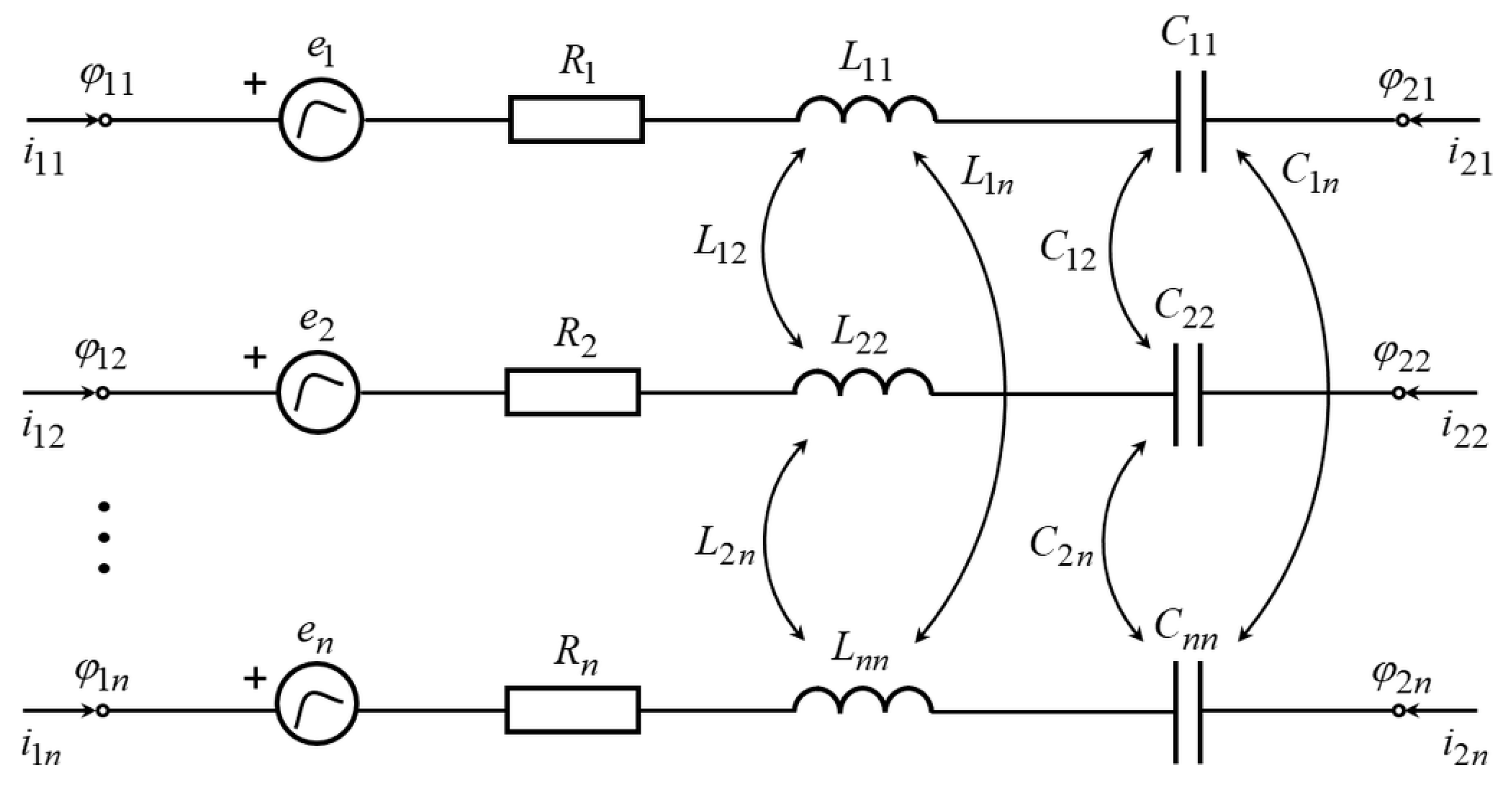
According to the FET terminology (based on the FEM approach), each circuit element can be defined as a single finite element (FE) with a corresponding local system of algebraic equations that are obtained in the time domain. The FE model of a coupled circuit finite element can be defined as a finite element with 2n local nodes as is shown in Figure 1, where ‘n’ is the number of coupled circuit element branches.

The coupled circuit finite element shown in Figure 1 is defined by the following system of coupled ordinary differential equations (ODE-s):

$$\left\{{\phi }_1\right\}-\left\{{\phi }_2\right\}=\left[R\right]\cdot \left\{i\right\}+\left[L\right]\cdot \frac{d\left\{i\right\}}{dt}+\left\{U_c\right\}+\left\{e\right\},$$

(1)

$$\left\{i\right\}=\left[C\right]\cdot \frac{d\left\{U_c\right\}}{dt},$$

(2)

where:

[R]—resistance matrix,

[L]—inductance matrix,

[C]—capacitance matrix,

{i₁}—nodal current vector of currents entering the finite element at local nodes ‘11’…‘1n’,

{i₂}—nodal current vector of currents entering the finite element at local nodes ‘21’…‘2n’,

{φ₁}—nodal potential vector at local nodes ‘11’…‘1n’,

{φ₂}—nodal potential vector at local nodes ‘21’…‘2n’,

{e}—electromotive force vector,

{U_c}—capacitance voltage vector.

2.1. Coupled Circuit Finite Element—Theta Method Time Integration Scheme

The general principles of the time integration of Equations (1) and (2) using the ϑ-method time integration scheme can be found in ref. [27]. To obtain a system of algebraic equations, it is necessary to perform a time integration of the system of coupled ODE-s (1) and (2):

$${\displaystyle \underset{t}{\overset{t+}{\int }}\left(\left\{{\phi }_1\right\}-\left\{{\phi }_2\right\}-\left[R\right]\cdot \left\{i\right\}-\left[L\right]\cdot \left\{\frac{di}{dt}\right\}-\left\{U_c\right\}-\left\{e\right\}\right)\cdot dt}=0,$$

(3)

$${\displaystyle \underset{t}{\overset{t+}{\int }}\left(\left\{i\right\}-\left[C\right]\cdot \frac{d\left\{U_c\right\}}{dt}\right)\cdot dt}=0.$$

(4)

The time integration based on the ϑ-method can be described by the following equations:

$${\displaystyle \underset{t}{\overset{t+}{\int }}f(t)\cdot dt\approx \left[\left(1-\vartheta \right)\cdot f+\vartheta \cdot f^{+}\right]\cdot \Delta t},$$

(5)

$${\displaystyle \underset{t}{\overset{t+}{\int }}\frac{df(t)}{dt}dt={\displaystyle \underset{t}{\overset{t+}{\int }}df(t)=}}{f}^{+}-f.$$

(6)

With the application of the ϑ-method on Equations (3) and (4), the following system of algebraic equations is obtained:

$$\begin{array}{l}{\left\{{\phi }_1\right\}}^{+}\cdot \vartheta \cdot \Delta t+\left\{{\phi }_1\right\}\cdot \left(1-\vartheta \right)\cdot \Delta t-{\left\{{\phi }_2\right\}}^{+}\cdot \vartheta \cdot \Delta t-\left\{{\phi }_2\right\}\cdot \left(1-\vartheta \right)\cdot \Delta t-\\ \left[R\right]\cdot {\left\{i\right\}}^{+}\cdot \vartheta \cdot \Delta t-\left[R\right]\cdot \left\{i\right\}\cdot \left(1-\vartheta \right)\cdot \Delta t-\left[L\right]\cdot {\left\{i\right\}}^{+}+\left[L\right]\cdot \left\{i\right\}-\\ {\left\{U_C\right\}}^{+}\cdot \vartheta \cdot \Delta t-\left\{U_C\right\}\cdot \left(1-\vartheta \right)\cdot \Delta t-{\left\{e\right\}}^{+}\cdot \vartheta \cdot \Delta t-\left\{e\right\}\cdot \left(1-\vartheta \right)\cdot \Delta t=0,\end{array}$$

(7)

$${\left\{U_c\right\}}^{+}={\left[C\right]}^{-1}\cdot {\left\{i\right\}}^{+}\cdot \vartheta \cdot \Delta t+{\left[C\right]}^{-1}\cdot \left\{i\right\}\cdot \left(1-\vartheta \right)\cdot \Delta t+\left\{U_c\right\}.$$

(8)

By including Equation (8) into Equation (7), the following system of equations is obtained:

$$\begin{array}{l}\vartheta \cdot \Delta t\cdot {\left\{{\phi }_1\right\}}^{+}+\left(1-\vartheta \right)\cdot \Delta t\cdot \left\{{\phi }_1\right\}-\vartheta \cdot \Delta t\cdot {\left\{{\phi }_2\right\}}^{+}-\left(1-\vartheta \right)\cdot \Delta t\cdot \left\{{\phi }_2\right\}-\\ \vartheta \cdot \Delta t\cdot \left[R\right]\cdot {\left\{i\right\}}^{+}-\left(1-\vartheta \right)\cdot \Delta t\cdot \left[R\right]\cdot \left\{i\right\}-\left[L\right]\cdot {\left\{i\right\}}^{+}+\left[L\right]\cdot \left\{i\right\}-\\ {\left(\vartheta \cdot \Delta t\right)}^2\cdot {\left[C\right]}^{-1}\cdot {\left\{i\right\}}^{+}-\left(\vartheta \cdot \Delta t\right)\cdot \left(1-\vartheta \right)\cdot \Delta t\cdot {\left[C\right]}^{-1}\cdot \left\{i\right\}-\\ \vartheta \cdot \Delta t\cdot \left\{U_c\right\}-\left(1-\vartheta \right)\cdot \Delta t\cdot \left\{U_c\right\}-\vartheta \cdot \Delta t\cdot {\left\{e\right\}}^{+}-\left(1-\vartheta \right)\cdot \Delta t\cdot \left\{e\right\}=0.\end{array}$$

(9)

Vectors marked by ‘+’ denote the variables’ state at the end of the time interval, while vectors without the mark denote the variables’ state at the beginning of the time interval Δt.

By separating the variables at the end of the time interval to the left-hand side and the variables at the beginning of the time interval to the right-hand side, the following system of equations is obtained:

$$\begin{array}{l}\left[\vartheta \cdot \Delta t\cdot \left[R\right]+\left[L\right]+{\left(\vartheta \cdot \Delta t\right)}^2{\left[C\right]}^{-1}\right]\cdot {\left\{i\right\}}^{+}=\vartheta \cdot \Delta t\cdot {\left\{{\phi }_1\right\}}^{+}-\\ \vartheta \cdot \Delta t\cdot {\left\{{\phi }_2\right\}}^{+}+\left(1-\vartheta \right)\cdot \Delta t\cdot \left\{{\phi }_1\right\}-\left(1-\vartheta \right)\cdot \Delta t\cdot \left\{{\phi }_2\right\}+\\ \left[-\left(1-\vartheta \right)\cdot \Delta t\cdot \left[R\right]+\left[L\right]-\left(\vartheta \cdot \Delta t\right)\cdot \left(1-\vartheta \right)\cdot \Delta t\cdot {\left[C\right]}^{-1}\right]\cdot \left\{i\right\}-\\ \vartheta \cdot \Delta t\cdot {\left\{e\right\}}^{+}-\left(1-\vartheta \right)\cdot \Delta t\cdot \left\{e\right\}-\Delta t\cdot \left\{U_c\right\}.\end{array}$$

(10)

Finally, the system of equations suitable for assembly procedure (FEM approach) can be defined as follows:

$$\begin{array}{l}\left[\begin{array}{cc}\left[B\right]& -\left[B\right]\\ -\left[B\right]& \left[B\right]\end{array}\right]\cdot \left[\begin{array}{c}\left\{{\phi }_1^{+}\right\}\\ \left\{{\phi }_2^{+}\right\}\end{array}\right]=\left[\begin{array}{cc}-\left[D\right]& \left[D\right]\\ \left[D\right]& -\left[D\right]\end{array}\right]\cdot \left[\begin{array}{c}\left\{{\phi }_1\right\}\\ \left\{{\phi }_2\right\}\end{array}\right]+\left[\begin{array}{c}\left[K\right]\\ -\left[K\right]\end{array}\right]\cdot \left\{U_c\right\}+\\ \left[\begin{array}{c}\left[D\right]\\ -\left[D\right]\end{array}\right]\cdot \left\{e\right\}+\left[\begin{array}{c}\left[B\right]\\ -\left[B\right]\end{array}\right]\cdot {\left\{e\right\}}^{+}+\left[\begin{array}{cc}-\left[H\right]& \left[0\right]\\ \left[0\right]& -\left[H\right]\end{array}\right]\cdot \left[\begin{array}{c}\left\{i_1\right\}\\ \left\{i_2\right\}\end{array}\right]+\left[\begin{array}{c}{\left\{i_1\right\}}^{+}\\ {\left\{i_2\right\}}^{+}\end{array}\right],\end{array}$$

(11)

where:

$$\left[A\right]=\vartheta \cdot \Delta t\cdot \left[R\right]+\left[L\right]+{\left(\vartheta \cdot \Delta t\right)}^2\cdot {\left[C\right]}^{-1},$$

(12)

$$\left[G\right]=-\left(1-\vartheta \right)\cdot \Delta t\cdot \left[R\right]+\left[L\right]-\left(\vartheta \cdot \Delta t\right)\cdot \left(1-\vartheta \right)\cdot \Delta t\cdot {\left[C\right]}^{-1},$$

(13)

$$\left[B\right]={\left[A\right]}^{-1}\cdot \vartheta \cdot \Delta t,$$

(14)

$$\left[D\right]={\left[A\right]}^{-1}\cdot \left(1-\vartheta \right)\cdot \Delta t,$$

(15)

$$\left[H\right]={\left[A\right]}^{-1}\cdot \left[G\right],$$

(16)

$$\left[K\right]=\Delta t\cdot {\left[A\right]}^{-1},$$

(17)

$${\left\{i_1\right\}}^{+}={\left\{i\right\}}^{+},$$

(18)

$${\left\{i_2\right\}}^{+}=-{\left\{i\right\}}^{+}.$$

(19)

2.2. Coupled Circuit Finite Element—Heun’s Method Time Integration Scheme

The general principles of the time integration of Equations (1) and (2) using Heun’s method time integration scheme can be found in ref. [28]. To perform the time integration according to Heun’s method, it is necessary to rewrite Equations (1) and (2) in the following form:

$$\frac{d\left\{i\right\}}{dt}=f_1\left(\left\{i\right\},\left\{U_c\right\},\left\{{\phi }_1\right\},\left\{{\phi }_2\right\},\left\{e\right\}\right),$$

(20)

$$\frac{d\left\{U_c\right\}}{dt}=f_2\left(\left\{i\right\}\right),$$

(21)

$$\begin{array}{l}{f}_1\left(\left\{i\right\},\left\{U_c\right\},\left\{{\phi }_1\right\},\left\{{\phi }_2\right\},\left\{e\right\}\right)=-{\left[L\right]}^{-1}\cdot \left[R\right]\cdot \left\{i\right\}+{\left[L\right]}^{-1}\cdot \left\{{\phi }_1\right\}-\\ -{\left[L\right]}^{-1}\cdot \left\{{\phi }_2\right\}-{\left[L\right]}^{-1}\cdot \left\{U_c\right\}-{\left[L\right]}^{-1}\cdot \left\{e\right\},\end{array}$$

(22)

$$f_2\left(\left\{i\right\}\right)={\left[C\right]}^{-1}\cdot \left\{i\right\}.$$

(23)

According to Heun’s method, the state of variables at the end of the time interval is defined by the following corrector equations:

$$\begin{array}{l}\left\{i^{+}\right\}=\left\{i\right\}+\frac{\Delta t}{2}\cdot f_1\left(\left\{i\right\},\left\{U_c\right\},\left\{{\phi }_1\right\},\left\{{\phi }_2\right\},\left\{e\right\}\right)+\\ \frac{\Delta t}{2}\cdot f_1\left({\left\{i^{+}\right\}}^p,\left\{U_c^{+}\right\},\left\{{\phi }_1^{+}\right\},\left\{{\phi }_2^{+}\right\},\left\{e^{+}\right\}\right),\end{array}$$

(24)

$$\left\{U_c^{+}\right\}=\left\{U_c\right\}+\frac{\Delta t}{2}\cdot f_2\left(\left\{i\right\}\right)+\frac{\Delta t}{2}\cdot f_2\left(\left\{i^{+}\right\}\right).$$

(25)

According to (22) and (23), the predicted slope of f₁({i⁺}^p, {U_c⁺}, {φ₁⁺}, { φ₂⁺}, {e⁺}) and f₂({i⁺}) at the end of the time interval are:

$$\begin{array}{l}{f}_1\left({\left\{i^{+}\right\}}^p,\left\{U_c^{+}\right\},\left\{{\phi }_1^{+}\right\},\left\{{\phi }_2^{+}\right\},\left\{e^{+}\right\}\right)=-{\left[L\right]}^{-1}\cdot \left[R\right]\cdot {\left\{i^{+}\right\}}^p+\\ {\left[L\right]}^{-1}\cdot \left\{{\phi }_1^{+}\right\}-{\left[L\right]}^{-1}\cdot \left\{{\phi }_2^{+}\right\}-{\left[L\right]}^{-1}\cdot \left\{U_c^{+}\right\}-{\left[L\right]}^{-1}\cdot \left\{e^{+}\right\},\end{array}$$

(26)

$$f_2\left(\left\{i^{+}\right\}\right)={\left[C\right]}^{-1}\cdot \left\{i^{+}\right\},$$

(27)

where {i⁺}^p is the predicted current value at the end of the time interval defined by the following predictor equation:

$${\left\{i^{+}\right\}}^p=\left\{i\right\}+\Delta t\cdot f_1\left(\left\{i\right\},\left\{U_c\right\},\left\{{\phi }_1\right\},\left\{{\phi }_2\right\},\left\{e\right\}\right),$$

(28)

where f₁({i}, {U_c}, {φ₁}, {φ₂}, {e}) is defined by (22).

Combining (24)–(28) and separating the variables at the end of the time interval to the left-hand side and the variables at the beginning of the time interval to the right-hand side, the following algebraic equations are obtained:

$$\begin{array}{l}\left\{i^{+}\right\}=\left\{i\right\}+\frac{\Delta t}{2}\cdot (\left\{{\phi }_1\right\}\cdot {\left[L\right]}^{-1}-\left\{{\phi }_2\right\}\cdot {\left[L\right]}^{-1}-\left[R\right]\cdot \left\{i\right\}\cdot {\left[L\right]}^{-1}-\\ \left\{U_c\right\}\cdot {\left[L\right]}^{-1}-\left\{e\right\}\cdot {\left[L\right]}^{-1})+\frac{\Delta t}{2}\cdot \left\{{\phi }_1^{+}\right\}\cdot {\left[L\right]}^{-1}-\frac{\Delta t}{2}\cdot \left\{{\phi }_2^{+}\right\}\cdot {\left[L\right]}^{-1}-\\ \frac{\Delta t}{2}\cdot \left[R\right]\cdot {\left[L\right]}^{-1}\cdot (\left\{i\right\}+\Delta t\cdot (\left\{{\phi }_1\right\}\cdot {\left[L\right]}^{-1}-\left\{{\phi }_2\right\}\cdot {\left[L\right]}^{-1}-\\ \left[R\right]\cdot \left\{i\right\}\cdot {\left[L\right]}^{-1}-\left\{U_c\right\}\cdot {\left[L\right]}^{-1}-\left\{e\right\}\cdot {\left[L\right]}^{-1}))-\\ \frac{\Delta t}{2}\cdot \left\{U_c^{+}\right\}\cdot {\left[L\right]}^{-1}-\frac{\Delta t}{2}\cdot \left\{e^{+}\right\}\cdot {\left[L\right]}^{-1},\end{array}$$

(29)

$$\left\{U_c^{+}\right\}=\left\{U_c\right\}+\frac{\Delta t}{2}\cdot \left\{i\right\}\cdot {\left[C\right]}^{-1}+\frac{\Delta t}{2}\cdot \left\{i^{+}\right\}\cdot {\left[C\right]}^{-1}.$$

(30)

By including Equation (30) into Equation (29), the following system of equations is obtained:

$$\begin{array}{l}\left\{i^{+}\right\}=\frac{\Delta t}{2}\cdot {\left[L\right]}^{-1}\cdot {\left(\left[I\right]+\frac{\Delta t^2}{4}\cdot {\left[L\right]}^{-1}\cdot {\left[C\right]}^{-1}\right)}^{-1}\cdot \left\{{\phi }_1^{+}\right\}-\\ \frac{\Delta t}{2}\cdot {\left[L\right]}^{-1}\cdot {\left(1+\frac{\Delta t^2}{4}\cdot {\left[L\right]}^{-1}\cdot {\left[C\right]}^{-1}\right)}^{-1}\cdot \left\{{\phi }_2^{+}\right\}+\\ \left(\frac{\Delta t}{2}\cdot {\left[L\right]}^{-1}-\frac{\Delta t^2}{2}\cdot \left[R\right]\cdot {\left[L\right]}^{-2}\right)\cdot {\left(1+\frac{\Delta t^2}{4}\cdot {\left[L\right]}^{-1}\cdot {\left[C\right]}^{-1}\right)}^{-1}\cdot \left\{{\phi }_1\right\}+\\ \left(\frac{\Delta t^2}{2}\cdot {\left[L\right]}^{-2}\cdot \left[R\right]-\frac{\Delta t}{2}\cdot {\left[L\right]}^{-1}\right)\cdot {\left(1+\frac{\Delta t^2}{4}\cdot {\left[L\right]}^{-1}\cdot {\left[C\right]}^{-1}\right)}^{-1}\cdot \left\{{\phi }_2\right\}+\\ \left(\frac{\Delta t^2}{2}\cdot {\left[L\right]}^{-2}\cdot \left[R\right]-\Delta t\cdot {\left[L\right]}^{-1}\right)\cdot {\left(1+\frac{\Delta t^2}{4}\cdot {\left[L\right]}^{-1}\cdot {\left[C\right]}^{-1}\right)}^{-1}\cdot \left\{U_c\right\}+\\ \left(-\frac{\Delta t}{2}\cdot {\left[L\right]}^{-1}\right)\cdot {\left(1+\frac{\Delta t^2}{4}\cdot {\left[L\right]}^{-1}\cdot {\left[C\right]}^{-1}\right)}^{-1}\cdot \left\{e^{+}\right\}+\\ \left(\frac{\Delta t^2}{2}\cdot {\left[L\right]}^{-2}\cdot \left[R\right]-\frac{\Delta t}{2}\cdot {\left[L\right]}^{-1}\right)\cdot {\left(1+\frac{\Delta t^2}{4}\cdot {\left[L\right]}^{-1}\cdot {\left[C\right]}^{-1}\right)}^{-1}\cdot \left\{e\right\}+\\ \left(1-\Delta t\cdot {\left[L\right]}^{-1}\cdot \left[R\right]+\frac{\Delta t^2}{2}\cdot {\left[L\right]}^{-2}\cdot {\left[R\right]}^2-\frac{\Delta t^2}{4}\cdot {\left[L\right]}^{-1}\cdot {\left[C\right]}^{-1}\right)\cdot \\ {\left(1+\frac{\Delta t^2}{4}\cdot {\left[L\right]}^{-1}\cdot {\left[C\right]}^{-1}\right)}^{-1}\cdot \left\{i\right\}.\end{array}$$

(31)

Finally, the system of equations suitable for assembly procedure (FEM approach) can be defined as follows:

$$\begin{array}{l}\left[\begin{array}{cc}\left[A\right]& \left[B\right]\\ -\left[A\right]& -\left[B\right]\end{array}\right]\cdot \left[\begin{array}{c}\left\{{\phi }_1^{+}\right\}\\ \left\{{\phi }_2^{+}\right\}\end{array}\right]=\left[\begin{array}{cc}-\left[D\right]& -\left[E\right]\\ \left[D\right]& \left[E\right]\end{array}\right]\cdot \left[\begin{array}{c}\left\{{\phi }_1\right\}\\ \left\{{\phi }_2\right\}\end{array}\right]+\left[\begin{array}{c}-\left[F\right]\\ \left[F\right]\end{array}\right]\cdot \left\{U_c\right\}+\\ \left[\begin{array}{c}-\left[H\right]\\ \left[H\right]\end{array}\right]\cdot \left\{e^{+}\right\}+\left[\begin{array}{c}-\left[K\right]\\ \left[K\right]\end{array}\right]\cdot \left\{e\right\}+\left[\begin{array}{cc}-\left[J\right]& \left[0\right]\\ \left[0\right]& -\left[J\right]\end{array}\right]\cdot \left[\begin{array}{c}\left\{i_1\right\}\\ \left\{i_2\right\}\end{array}\right]+\left[\begin{array}{c}{\left\{i_1\right\}}^{+}\\ {\left\{i_2\right\}}^{+}\end{array}\right],\end{array}$$

(32)

$$\left[G\right]=\left[I\right]+\frac{\Delta t^2}{4}\cdot {\left[L\right]}^{-1}\cdot {\left[C\right]}^{-1},$$

(33)

$$\left[A\right]=\frac{\Delta t}{2}\cdot {\left[G\right]}^{-1}\cdot {\left[L\right]}^{-1},$$

(34)

$$\left[B\right]=-\frac{\Delta t}{2}\cdot {\left[G\right]}^{-1}\cdot {\left[L\right]}^{-1},$$

(35)

$$\left[D\right]=\frac{\Delta t}{2}\cdot {\left[G\right]}^{-1}\cdot {\left[L\right]}^{-1}-\frac{\Delta t^2}{2}\cdot {\left[G\right]}^{-1}\cdot {\left[L\right]}^{-2}\cdot \left[R\right],$$

(36)

$$\left[E\right]=-\frac{\Delta t}{2}\cdot {\left[G\right]}^{-1}\cdot {\left[L\right]}^{-1}+\frac{\Delta t^2}{2}\cdot {\left[G\right]}^{-1}\cdot {\left[L\right]}^{-2}\cdot \left[R\right],$$

(37)

$$\left[F\right]=-\Delta t\cdot {\left[G\right]}^{-1}\cdot {\left[L\right]}^{-1}+\frac{\Delta t^2}{2}\cdot {\left[G\right]}^{-1}\cdot {\left[L\right]}^{-2}\cdot \left[R\right],$$

(38)

$$\left[H\right]=\frac{\Delta t}{2}\cdot {\left[G\right]}^{-1}\cdot {\left[L\right]}^{-1},$$

(39)

$$\left[K\right]=-\frac{\Delta t}{2}\cdot {\left[G\right]}^{-1}\cdot {\left[L\right]}^{-1}+\frac{\Delta t^2}{2}\cdot {\left[G\right]}^{-1}\cdot {\left[L\right]}^{-2}\cdot \left[R\right],$$

(40)

$$\begin{array}{l}\left[J\right]={\left[G\right]}^{-1}-\Delta t\cdot {\left[G\right]}^{-1}\cdot {\left[L\right]}^{-1}\cdot \left[R\right]+\\ \vartheta \cdot \Delta t^2\cdot {\left[G\right]}^{-1}\cdot {\left[L\right]}^{-2}\cdot {\left[R\right]}^2-\frac{\Delta t^2}{4}\cdot {\left[G\right]}^{-1}\cdot {\left[L\right]}^{-1}\cdot {\left[C\right]}^{-1},\end{array}$$

(41)

$${\left\{i_1\right\}}^{+}={\left\{i\right\}}^{+},$$

(42)

$${\left\{i_2\right\}}^{+}=-{\left\{i\right\}}^{+}.$$

(43)

2.3. Assembling Procedure

The general principles of the FET assembling procedure based on the FEM approach can be found in refs. [27,28]. To perform the assembling procedure, local systems (11) in the case of the ϑ-method time integration scheme and (32) in the case of Heun’s method time integration scheme, each FE has to be set in the following form:

$$\left\{\begin{array}{c}{\left\{i_1\right\}}^{+}\\ {\left\{i_2\right\}}^{+}\end{array}\right\}=\left[Q\right]\cdot \left\{\begin{array}{c}{\left\{{\phi }_1\right\}}^{+}\\ {\left\{{\phi }_2\right\}}^{+}\end{array}\right\}+\left\{\begin{array}{c}{F}_1\left(\left\{{\phi }_1\right\},\left\{{\phi }_2\right\},\left\{i_1\right\},\left\{i_2\right\}\right)\\ F_2\left(\left\{{\phi }_1\right\},\left\{{\phi }_2\right\},\left\{i_1\right\},\left\{i_2\right\}\right)\end{array}\right\}.$$

(44)

The global system must be solved for each time step, evaluating unknown nodal potentials. The value of the current of each finite element is then computed using relation (44) for each time step.

3. Numerical Example

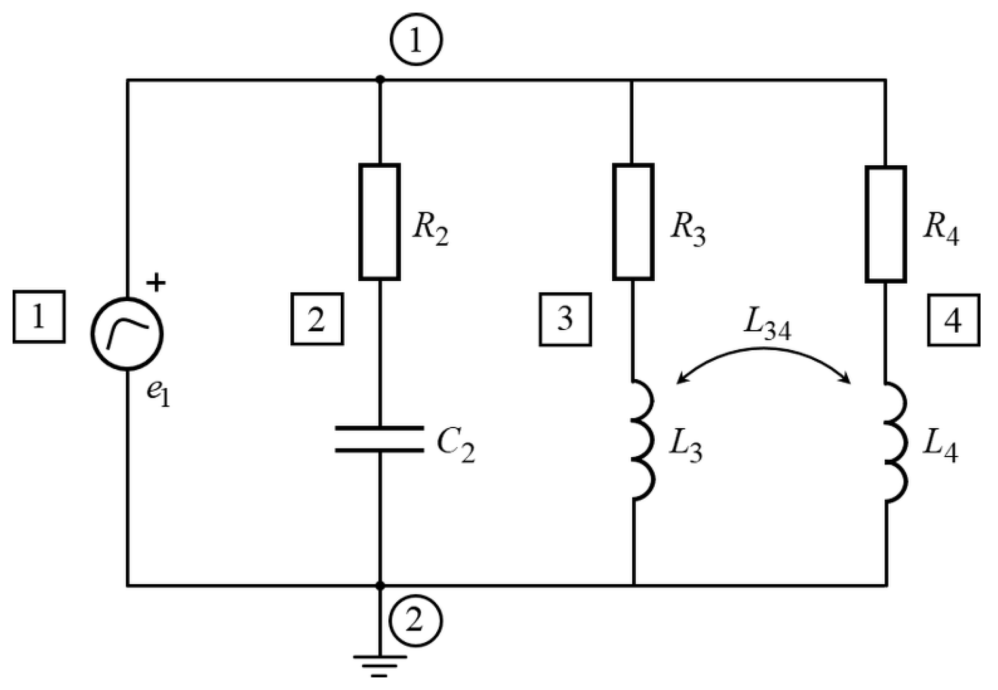
To present the basic principle of the developed FET-based algorithm and to perform transient analysis, the following coupled linear circuit was analyzed.

A coupled linear electrical circuit, shown in Figure 2 has four branches and two global nodes.

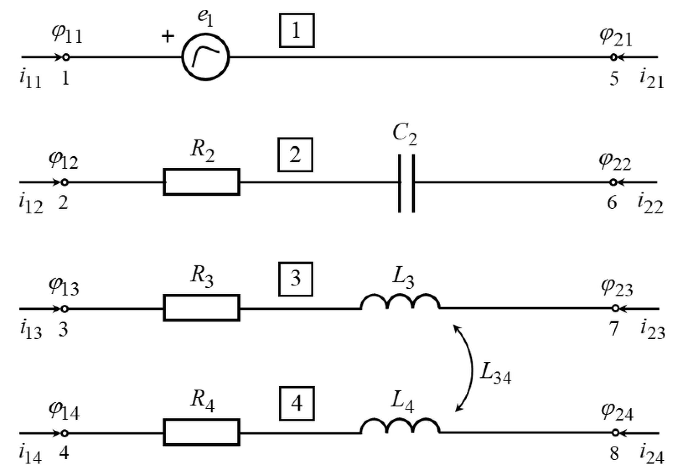
Figure 3 shows the entire coupled linear circuit as a unique finite element (FE) prepared for the FET procedure. It has eight local nodes and four branches. The first branch contains an electromotive force that is a ramp function (in the time interval 0–100 ms increases its value from 0 up to 10 V). The value of the time interval Δt was taken as 0.1 ms. The values of the circuit elements were assumed to be as follows: R₂ = 1 Ω, R₃ = 2 Ω, R₄ = 1 Ω, C₂ = 1 mF, L₃ = 0.1 H, L₄ = 0.01 H, L₃₄ = 0.1 mH.

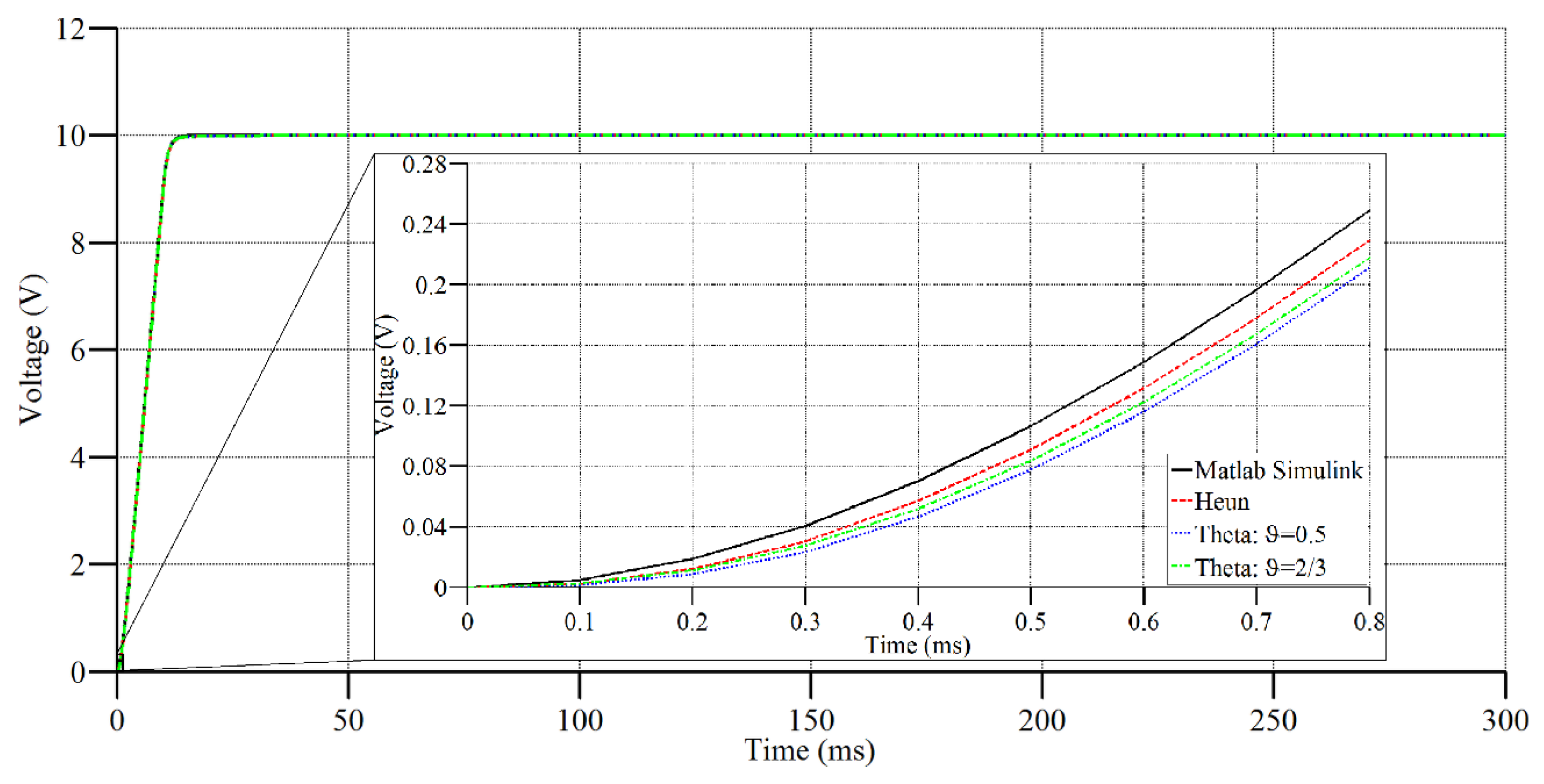
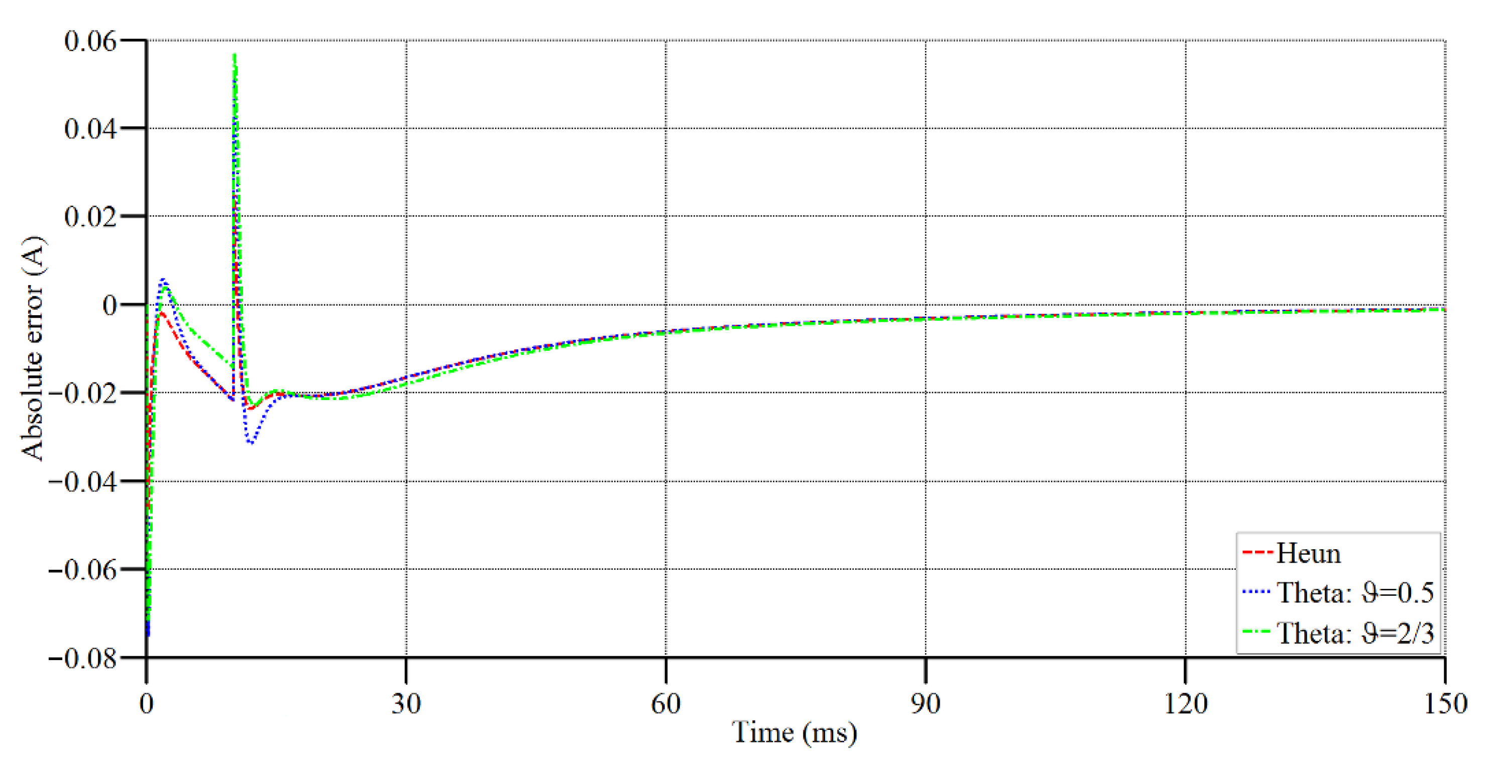
Figure 4 shows the current in the first branch during the 0–0.6 ms time interval as well as during the entire simulation while Figure 5 shows the second branch capacitor voltage during the 0–0.8 ms time interval, as well as during the entire simulation. Numerical solutions obtained using Heun’s method and using the generalized trapezoidal rule were compared to the solution obtained by Matlab Simulink software.

Absolute errors of numerical solutions related to the Matlab Simulink solution are shown in Figure 6 and Figure 7. Maximum values of these errors are presented numerically in

Table 1. Maximum absolute errors of the current in the first branch and capacitor voltage in the second branch.

Methods	Current	Capacitor Voltage
Heun	0.046789	0.033552
Theta: ϑ = 0.5	0.074807	0.041031
Theta: ϑ = 2/3	0.071435	0.034416

.

It was shown that the accuracy of results depends on the type of time integration scheme when performing the FET procedure. The above examples clearly show that time integration obtained by Heun’s integration scheme gives a higher accuracy of results compared with results obtained by the generalized trapezoidal rule (ϑ-method). The problem when using the ϑ-method is the fact that the accuracy of results highly depends on the chosen time integration parameter value.

4. Conclusions

In this paper, a novel algorithm for a transient linear circuit analysis based on the Finite Element Technique (FET) was established. The FET procedure allows a straightforward solution of complex electric circuits since it is based on the Finite Element Method (FEM) approach. Using an assembling procedure based on the FEM approach, it is quite straightforward to develop a numerical model of a complex electric circuit by focusing on the modeling of a single element in a linear electric circuit. The algorithm allows us to choose various types of time integration schemes when forming a local system of equations for a coupled circuit finite element. In this paper, a local system of equations of a coupled circuit finite element was obtained using the generalized trapezoidal rule (ϑ-method) as well as using Heun’s method.

To show the basic principle of the developed FET-based algorithm and to perform transient analysis, the random coupled linear circuit was analyzed. Numerical solutions obtained using Heun’s method and using the generalized trapezoidal rule were compared to the solution obtained by Matlab Simulink software. It was shown that the accuracy of results depends on the type of time integration scheme when performing the FET procedure. In the case of Heun’s method and ϑ-method time integration scheme, higher accuracy was obtained using Heun’s method.

References

- Nagel, L.W. SPICE2: A Computer Program to Simulate Semiconductor Circuits. Ph.D. Dissertation, University of California, Berkeley, Berkeley, CA, USA, 1975. Tech. Rep. UCB/ERL M520. [Google Scholar]
- Devgan, A.; Rohrer, R.A. Event driven adaptively controlled explicit simulation of integrated circuits. In Proceedings of the International Conference on Computer-Aided Design, Santa Clara, CA, USA, 7–11 November 1993; pp. 136–140. [Google Scholar]
- Dong, W.; Li, P.; Ye, X. Wavepipe: Parallel transient simulation of analog and digital circuits on multi-core shared-memory machines. In Proceedings of the Design Automation Conference, Anaheim, CA, USA, 8–13 June 2008; pp. 238–243. [Google Scholar]
- Dong, W.; Li, P. Parallelizable stable explicit numerical integration for efficient circuit simulation. In Proceedings of the Design Automation Conference, San Francisco, CA, USA, 26–31 July 2009; pp. 382–385. [Google Scholar]
- Griffith, R.; Nakhla, M. A new high-order absolutely-stable explicit numerical integration algorithm for the time-domain simulation of nonlinear circuits. In Proceedings of the International Conference on Computer-Aided Design, San Jose, CA, USA, 9–13 November 1997; pp. 276–280. [Google Scholar]
- Lelarasmee, E.; Ruehli, A.E.; Sangiovanni-Vincentelli, A.L. The waveform relaxation method for time-domain analysis of large scale integrated circuits. IEEE Trans. Comput.-Aided Des. 1982, 1, 131–145. [Google Scholar] [CrossRef]
- Peng, H.; Cheng, C.-K. Parallel transistor level full-chip circuit simulation. In Proceedings of the Design, Automation & Test in Europe Conference, Nice, France, 20–24 April 2009; pp. 304–307. [Google Scholar]
- Schutt-Aine, J.E. Latency insertion method (LIM) for the FST transient simulation of large networks. IEEE Trans. Circuits Syst. I 2001, 48, 81–89. [Google Scholar] [CrossRef]
- Sekine, T.; Asai, H. Generalized leapfrog scheme for large-scale circuit simulation. In Proceedings of the IEEE Electrical Performance of Electronic Packaging and Systems, San Jose, CA, USA, 19–21 October 2009; pp. 81–84. [Google Scholar]
- Ye, X.; Dong, W.; Li, P.; Nassif, S. MAPS: Multi-algorithm parallel circuit simulation. In Proceedings of the IEEE International Conference on Computer-Aided Design, San Jose, CA, USA, 10–13 November 2008; pp. 73–78. [Google Scholar]
- Zhu, Z.; Shi, R.; Cheng, C.-K.; Kuh, E.S. An unconditional stable general operator splitting method for transistor level transient analysis. In Proceedings of the Asia and South Pacific Design Automation Conference, Yokohama, Japan, 24–27 January 2006; pp. 428–433. [Google Scholar]
- Tischendorf, C. Solution of Index-2 Differential Algebraic Equations and Its Application in Circuit Simulation. Ph.D. Thesis, Humboldt University, Berlin, Germany, 1996. [Google Scholar]
- Houben, S.H.M.J. Circuits in motion: The numerical simulation of electrical oscillators. Ph.D. Thesis, Technische Universiteit Eindhoven, The Netherlands, 2003. [Google Scholar]
- Hosea, M.E.; Shampine, L.F. Analysis and implementation of TR-BDF2. Appl. Numer. Math. 1996, 20, 21–37. [Google Scholar] [CrossRef]
- Swart, J.J.B. Parallel Software for Implicit Differential Equations. Ph.D. Thesis, University of Amsterdam, Amsterdam, The Netherlands, 1997. [Google Scholar]
- Günther, M.; Rentrop, P.; Feldmann, U. CHORAL—A one step method as numerical low pass filter in electrical network analysis. In Scientific Computing in Electrical Engineering; Springer: Berlin/Heidelberg, Germany, 2001; pp. 199–215. [Google Scholar] [CrossRef]
- Bruin, S.M.A. Modified Extended BDF Applied to Circuit Equations. M.S. Thesis, Vrije Universiteit Amsterdam, Amsterdam, The Netherlands, 2001. Nat. Lab. Unclassified Report 2001/826. [Google Scholar]
- Brugnano, L.; Trigiante, D. Solving Differential Problems by Multistep Initial and Boundary Value Methods; Gordon and Breach Science Publishers: Amsterdam, The Netherlands, 1998. [Google Scholar]
- Iavernaro, F.; Mazzia, F. Generalization of backward differentiation formulas for parallel computers. Numer. Algorithms 2002, 31, 139–155. [Google Scholar] [CrossRef]
- Zienkiewicz, O.C.; Taylor, R.L. The Finite Element Method, Volume 1: The Basis, 4th ed.; McGraw-Hill: Maidenhead, UK, 1989. [Google Scholar]
- Abo-Dahab, S.; Abbas, I.A. On the numerical solution of thermal shock problem for generalized magneto-thermoelasticity for an infinitely long annular cylinder with variable thermal conductivity. J. Comput. Theor. Nanosci. 2014, 11, 607–618. [Google Scholar] [CrossRef]
- Li, C.; Guo, H.; He, T.; Tian, X. Thermally nonlinear non-Fourier piezoelectric thermoelasticity problems with temperature-dependent elastic constants and thermal conductivity and nonlinear finite element analysis. Waves Random Complex Media 2022, 1–38. [Google Scholar] [CrossRef]
- Rahbar, H.; Javanbakht, M.; Ziaei-Rad, S.; Reali, A.; Jafarzadeh, H. Finite element analysis of coupled phase-field and thermoelasticity equations at large strains for martensitic phase transformations based on implicit and explicit time discretization schemes. Mech. Adv. Mater. Struc. 2021, 29, 2531–2547. [Google Scholar] [CrossRef]
- Mohamed, R.A.; Abbas, I.A.; Abo-Dahab, S. Finite element analysis of hydromagnetic flow and heat transfer of a heat generation fluid over a surface embedded in a non-Darcian porous medium in the presence of chemical reaction. Comm. Nonlinear Sci. Numer. Simul. 2009, 14, 1385–1395. [Google Scholar] [CrossRef]
- Moradnouri, A.; Vakilian, M.; Hekmati, A.; Fardmanesh, M. The end part of cryogenic H. V. bushing insulation design in a 230/20 kV HTS transformer. Cryogenics 2020, 108, 103090. [Google Scholar] [CrossRef]
- Attar, H.; Moradnouri, A.; Mirghaforian, R.; Hekmati, A. Impact of the radius of double pancake windings on the electromagnetic Behavior of high temperature superconducting transformer. COMPEL 2022, 41, 1753–1770. [Google Scholar] [CrossRef]
- Lucić, R.; Jurić-Grgić, I.; Kurtović, M. Time domain finite element method analysis of multi-conductor transmission lines. Euro. Trans. Electr. Power 2010, 20, 822–832. [Google Scholar] [CrossRef]
- Jurić-Grgic, I.; Lucic, R.; Krolo, I. Improving time integration scheme for FEM analysis of MTL problems. Int. J. Circuit Theory Appl. 2019, 47, 1800–1811. [Google Scholar] [CrossRef]
- Chapra, S.C.; Canale, R.C. Numerical Methods for Engineers, 7th ed.; McGraw-Hill: New York, NY, USA, 2015. [Google Scholar]