Article

Unfrozen Skewed Turbulence for Wind Loading on Structures

by
Etienne Cheynet
1,*,
Nicolò Daniotti
2,
Jasna Bogunović Jakobsen
2,
Jónas Snæbjörnsson
2,3 and
Jungao Wang
2,4
1
Geophysical Institute and Bergen Offshore Wind Centre (BOW), University of Bergen, 5007 Bergen, Norway
2
Department of Mechanical and Structural Engineering and Materials Science, University of Stavanger, 4036 Stavanger, Norway
3
Department of Engineering, Reykjavík University, Menntavegur 1, 101 Reykjavík, Iceland
4
Norwegian Public Roads Administration, Bergelandsgata 30, 4012 Stavanger, Norway
*
Author to whom correspondence should be addressed.
Appl. Sci. 2022, 12(19), 9537; https://doi.org/10.3390/app12199537
Submission received: 1 August 2022 / Revised: 17 September 2022 / Accepted: 17 September 2022 / Published: 22 September 2022

Abstract

:

Featured Application

This manuscript deals with the generation of turbulence wind histories with spatio-temporal characteristics suitable for the calculation of skewed wind dynamic load on slender structures. Such simulations may become essential for the design of future long-span bridges and high-rise buildings. The results presented are considered valuable in the field of structural engineering, boundary layer meteorology and computational wind engineering.

Abstract

The paper introduces an algorithm to generate a three-variate four-dimensional wind turbulence field suited for yawed wind dynamic load simulation. At large yaw angles, a relaxation of Taylor’s hypothesis of frozen turbulence becomes relevant as well as the flow phase lag in the along-wind direction, which modulates the real and imaginary parts of the coherence. To capture such a general wind action on a structure, a modified spectral representation method is used where the coherence of turbulence is described as a complex-valued function. The one-point and two-point co-spectra are implemented in the simulation setup using a square-root-free Cholesky decomposition of the spectral matrix. The numerical procedure is illustrated based on turbulence characteristics derived from data collected during storm Aina (2017) on the Norwegian coast by three-dimensional sonic anemometers. During this event, a remarkable 3-hour stationary time series with a mean wind speed of 24 m s 1 at a height of 49 m above ground was recorded. Since no computational grid is needed, the velocity fluctuations with representative spatio-temporal characteristics can be directly simulated on structural elements of slender structures. Such an algorithm may be essential for the design of super-long span bridges in coastal areas.

1. Introduction

In wind engineering, the yaw angle defines the angle between the wind direction and the line normal to the bridge deck in a horizontal plane. Flows associated with non-zero yaw angles are described as “skewed” and can influence the buffeting response of long-span bridges [1,2]. Wind tunnel tests on full aeroelastic models suggest that the largest turbulent load is not always associated with a zero yaw angle [2,3,4]. The aerodynamic characteristics of a bridge deck depend indeed on both the yaw angle and the angle of attack [5,6]. At large yaw angles, the mean wind velocity component normal to the main span is reduced, while the eddies no longer impinge the structure in multiple locations simultaneously but at different times. This leads to a modification of the spatial distribution of the oncoming gusts along the deck and thus a modification of the span-wise correlation of the turbulent loading. Therefore, for slender decks, the so-called strip assumption [7,8], which assumes that the along-span correlation of the wind-induced surface pressure fluctuations is not affected by the structure, may have to be reassessed even more carefully. Also, the turbulent flow characteristics in the along-wind and cross-wind direction differ significantly [9,10] such that their projection onto a bridge-based coordinate system will result in different fluctuating loadings, depending on the yaw angle.
Although some authors (e.g., [11,12]) discussed different approaches to model the buffeting load for a non-zero yaw angle, few studies describe the two-point turbulence characteristics in skewed flow conditions, especially for load computations in the time domain. Yet, such a description may become crucial to model the dynamic wind loading on slender structures such as long-span bridges, inclined stay cables [13,14] or wind turbines, which are sensitive to yaw errors [15]. Whereas the wind direction along a bridge is largely governed by the topography, the variability of the wind direction due to earth rotation, i.e., the direction shear, concerns the design of tall vertical structures. Recent studies have highlighted the influence of the direction shear on wind turbine performances [16] but also on the wind loading on high-rise buildings [17,18].
The coherence of turbulence is a correlation function in the frequency space that reflects the spatial distributions of eddies. At a given distance, larger eddies are more correlated than smaller ones. Therefore, the coherence decreases when the distance or the wavenumber increases. The coherence is at the heart of the dynamic wind load modelling for the design of structures.
The so-called root-coherence is the normalized cross-spectral density of turbulence fluctuations and is a complex-valued function. In the frequency space, the turbulent characteristics of skewed flows are addressed in the ESDU 86010 standard [19], where the imaginary part of the root-coherence becomes non-negligible. This reflects the fact that eddies impinge on different parts of a structure at different times (Figure 1). Taylor’s hypothesis of frozen turbulence [20] assumes that the same eddy moving in the streamwise direction at a speed u ¯ will be characterized by no loss of correlation except due to the time lag Δ t = d x / u ¯ , where d x is the streamwise separation (Figure 1). Turbulence may no longer be considered frozen if the streamwise distance becomes large compared to a typical length scale of turbulence. ESDU [19] relaxes Taylor’s hypothesis by modelling the root-coherence in the along-wind direction, albeit with parameters that can deviate substantially from those found in the literature [10,21,22].
The present study introduces an algorithm to generate a three-variate four-dimensional correlated wind field in the time domain, which accounts for non-zero yaw angles and non-frozen turbulence. The turbulence generator relies on a spectral representation approach [23], i.e., it requires knowledge of the one-point and two-point power spectral densities (PSDs) of the velocity fluctuations. The term three-variate refers to three velocity components of the wind field, whereas the term four-dimensional refers here to the three spatial dimensions plus the temporal one. To further ensure a realistic flow simulation, the correlation between the vertical and along-wind components is modelled using a negative cross-spectral density. The suitability of the algorithm is illustrated by simulations, based on the turbulence characteristics derived from velocity records from storm Aina (2017). The measurement data were collected by three sonic anemometers mounted on a 50-m high mast in the Bjørnafjord on the Norwegian coast. According to the E39 Coastal Highway Route project, the fjord will be crossed by a 5-km floating pontoon bridge [24], motivating the development of a more realistic flow simulation for improved wind load calculation. In particular, recent wind tunnel tests for this bridge have shown that accounting for skewed wind conditions is highly valuable [25].
The dataset used in the present study illustrates the feasibility of the turbulence generator as well as the use of surface layer scaling to parametrize the flow conditions. The study of the dynamic response of a large structure to a skewed turbulent field is, however, clearly beyond the scope of the present paper and will not be addressed hereinafter. Finally, it should be noted that spectral methods to simulate random processes with phase delays between different locations have been used in the past for ground acceleration records (e.g., [26,27]). However, the time scales involved in earthquake simulations are around 30 s against 600 s to 3600 s for atmospheric turbulence simulation, i.e., one to two orders of magnitude smaller. Therefore, the method presented herein is hardly comparable with those used in earthquake engineering.
The present paper is organised as follows: Section 2 describes the spectral flow characteristics and scaling laws adopted to simulate a skewed turbulent field with unfrozen turbulence relevant to wind load modelling on a long-span floating bridge. Section 3 introduces the algorithm to generate wind turbulence with a complex-valued root-coherence function, reflecting the phase lag of the wind velocity fluctuations. Section 4.1 illustrates the suitability of the selected spectral flow characteristics by using them to characterize the turbulent flow field recorded during storm Aina. The fitted turbulence parameters are adopted in Section 5.1 to illustrate the performances of the proposed algorithm by generating a realistic turbulent wind field for a simplified geometry.

2. Materials and Methods

2.1. Surface Layer Turbulence Modelling

The flow characteristics are modelled using surface-layer scaling as described by Monin and Obukhov [28] and Kaimal et al. [29], where the scaling velocity is the friction velocity u * and the controlling length scale is the height z above the surface. This approach is appropriate for a fjord-crossing bridge, for which the deck is located within the first 80 m above ground or sea surface. The three velocity components are denoted u, v and w and refer to the along-wind (x-axis), the cross-wind (y-axis) and the vertical components (positive z-axis), respectively. One shall assume that each velocity component i = u , v , w can be decomposed into a mean component i ¯ and a fluctuating component i with zero mean, which is a stationary, ergodic and Gaussian random process. The standard deviation of the u, v and w components are denoted σ u , σ v and σ w , respectively. The associated turbulence intensities are I u = σ u / u ¯ , I v = σ v / u ¯ and I w = σ w / u ¯ .
Surface-layer scaling allows the generation of a turbulent wind field knowing the friction velocity u * , the roughness length z 0 , the reference mean wind speed u ¯ r e f at a reference height z r e f , the normalized velocity spectra f S i j / u * 2 , where ( i , j ) = u , v , w and the root-coherence of turbulence. To generate a four-dimensional flow, the root-coherence needs to be characterized for the along-wind, cross-wind and vertical directions. The values of σ u , σ v and σ w are not explicitly required as they are governed by the terrain roughness z 0 and can be retrieved by integrating the velocity spectra over the frequencies. The present approach does not need the integral turbulence length scales either, which is in general advantageous for studies relying on measurements in the natural wind. The integral turbulence length scales are significantly affected by the low-frequency velocity fluctuations which can be predominant in an outdoor environment. Therefore, the integral turbulence length scales are commonly estimated with large uncertainties. Panofsky and Dutton [30] (pp. 175–176) even recommend avoiding them in studying the properties of atmospheric turbulence.

2.2. One-Point Velocity Spectra

The spectral characteristics of turbulence are described herein for a neutral atmosphere, which is dominating under strong wind conditions (see e.g., [31]). The one-point power spectral densities of the velocity fluctuations S i ( f , x , y , z ) , ( i ) = u , v , w are functions of both the frequency f and the location ( x , y , z ) . For the sake of brevity, only the dependency on f is explicitly shown herein. The target power spectral densities for the horizontal and vertical wind components are modelled using the so-called “blunt” and “pointed” models, respectively [32,33]
f S u ( f ) u * 2 = a u f r 1 + b u f r 5 / 3
f S v ( f ) u * 2 = a v f r 1 + b v f r 5 / 3
f S w ( f ) u * 2 = a w f r 1 + b w f r 5 / 3
where f r = f z / u ¯ is a reduced frequency; a i and b i , with i = u , v , w , are coefficients empirically estimated. For a neutral atmosphere, the hypothesis of local isotropy in the inertial subrange [34] can be used to reduce the number of parameters in Equations (1) to (3). The assumption, already exploited by Kaimal et al. [29], means that f S u ( f ) / u * 2 0.3 f r 2 / 3 , f S v ( f ) / u * 2 0.4 f r 2 / 3 and f S w ( f ) / u * 2 0.4 f r 2 / 3 at f r 1 . This implies that b u = ( a u / 0.3 ) 3 / 5 , b v = ( a v / 0.4 ) 3 / 5 and b w = a w / 0.4 . As a result, the following relation is obtained [34]:
S w S u S v S u 4 3 at f r 1
The above relationship is generally observed for the neutral atmosphere and is a necessary condition for realistic 3D flow simulation in the near-neutral atmospheric surface layer [29,35,36]. Another interesting property of Equation (1) is that the maximal value of the normalized spectrum S u is reached at a frequency f k such that
f k S u ( f k ) u * 2 1
To account properly for the covariance between the u and w components, the co-spectrum between the longitudinal and vertical velocity components needs to be modelled. The co-spectrum, which is the real part of the cross-spectrum, is denoted C o u w . Defining the friction velocity as
u * = u w ¯ ,
the co-spectrum can be modelled using a similar expression as that used by Kaimal et al. [29]:
f C o u w ( f ) u * 2 = a u w f r 1 + b u w f r 7 / 3
where a u w and b u w are two constants to be determined empirically. The above definition of the friction velocity implies that v w ¯ 0 and thus S v w 0 . Although this may not always be observed in full-scale [37], it is a reasonable approximation for modelling purposes. Similarly, it is generally assumed that the co-spectral estimate S u v has negligible values such that turbulent momentum fluxes are driven by the vertical wind component only. If the friction velocity is defined as in Equation (6), the integration of Equation (7) over the frequencies should be equal to u * 2 , which implies that b u w = 3 / 4 a u w . Kaimal et al. [29] studied the friction velocity based on the work of Haugen et al. [38], which defined u * as in Equation (6). However, they obtained a u w = 14.0 and b u w = 9.6 , i.e., b u w 0.69 a u w . Therefore, to simulate correlated turbulent wind histories with consistent values between the target and computed friction velocity, the co-spectrum proposed by Kaimal et al. [29] was not used directly. Instead a modified co-spectrum formulation with b u w = 3 / 4 a u w is chosen. The coefficient a u w can be obtained by modifying the value used by Kaimal et al. [29] or by fitting Equation (7) to the co-spectrum estimated using measurement data.
For a structure above the sea surface, the surface friction velocity ( u * ) 0 can be estimated using Charnock’s wind stress formula [39]. Onshore, in flat terrain, ( u * ) 0 can be derived from the logarithmic profile in the neutral atmospheric surface layer:
( u * ) 0 = u ¯ r e f κ log ( z r e f / z 0 )
where κ 0.40 is the von Kármán constant [40]; u ¯ r e f is the mean wind speed at a reference height z r e f , which is typically a few meters above the surface. For the sake of simplicity, the surface friction velocity is here assumed constant with the height in the surface layer, i.e., the first 10% of the atmospheric boundary layer, such that u * ( u * ) 0 . The classical logarithmic mean wind speed profile can then be retrieved as
u ¯ ( z ) = ( u * ) 0 κ log ( z / z 0 )
Equation (9) is applicable if the boundary layer is in equilibrium near the surface, which is not always the case for natural flows. Depending on the terrain uniformity, the mean flow characteristics can be derived from micro-scale numerical models (e.g., [41]). When appropriate, the mean wind speed profile from state-of-the-art open-access wind atlases [42,43] can also be used.
Although the content of the present section is well established in micro-meteorology, many wind field simulations used for engineering applications do not verify Equation (4). To the author’s knowledge, Equation (7) is usually included for frequency-domain analysis (e.g., [44]) but not time-domain analysis, where the wind loading can be non-linear. Finally, it should be noted that the use of u * as scaling velocity implies that σ w / σ u or σ v / σ u are height-dependant, as recommended by ESDU [45], whereas it is not the case in EN 1991-1-4 [46] or in the Handbook N400 [47]. Although this height-dependency is rather small at altitudes between 30 m and 100 m above the surface, it may not be negligible for floating pontoon bridges, the deck height of which is between 10 m and 20 m above the surface.

2.3. Taylor’s Hypothesis of Frozen Turbulence

Taylor’s hypothesis of frozen turbulence [20] assumes that eddies are unchanged as they are advected in the mean flow direction. This hypothesis is generally applicable if the along-wind component is characterized by a low turbulence intensity. In practice, this hypothesis is used to relate temporal averaging and spatial averaging [48]. The applicability of Taylor’s hypothesis is, however, scale-dependent [49] and is generally adequate for large eddies, i.e., at low wave-numbers only [50,51].
The limit of Taylor’s hypothesis needs to be accounted for in modelling skewed wind loads, if the flow field stretches over large distances, e.g., 2 k m for existing cable-suspended bridges. At such large separations, the eddies impinging the structure are not only characterized by a phase difference (Figure 1) but also a loss of correlation in the streamwise direction. This loss of correlation can be conveniently modelled using a root-coherence model for along-wind separation, also called longitudinal distances [30,52]. Although this approach relaxes Taylor’s hypothesis without fully correcting it, it is a convenient tool for wind engineering applications and has also been previously used in fundamental science [53]. Besides, recent progress in pulsed lidar remote sensing of wind has also given new opportunities to study and model the along-wind root-coherence based on the simultaneous flow recordings in multiple positions [22,54,55,56,57].
In the present wind field simulation procedure, we first and foremost aim to account for the out-of-phase velocity fluctuations due to skewed wind direction. The relaxation of Taylor’s hypothesis is a further refinement toward a more realistic flow simulation. As a limit case, frozen turbulence can be recovered by simply forcing the longitudinal root-coherence to be equal to one at every frequency.

2.4. Coherence Modelling

The root-coherence between two velocity components i and j, where i , j = u , v , w and between two points located at coordinates x 1 , y 1 , z 1 and x 2 , y 2 , z 2 is defined as
coh i j ( f , x 1 , y 1 , z 1 , x 2 , y 2 , z 2 ) = S i j ( f , x 1 , y 1 , z 1 , x 2 , y 2 , z 2 ) S i ( f , x 1 , y 1 , z 1 ) S j ( f , x 2 , y 2 , z 2 ) ,
where S i j ( f , x 1 , y 1 , z 1 , x 2 , y 2 , z 2 ) is the two-point cross-spectral density between the i and j components; S i ( f , x 1 , y 1 , z 1 ) and S j ( f , x 2 , y 2 , z 2 ) are the one-point spectra estimated at coordinates x 1 , y 1 , z 1 and x 2 , y 2 , z 2 , respectively. For the sake of simplicity, the root-coherence is assumed to be a function of the spatial separations rather than the measurement locations, i.e.,
coh i j ( f , x 1 , y 1 , z 1 , x 2 , y 2 , z 2 ) coh i j ( f , d x , d y , d z ) ,
where d x = x 1 x 2 , d y = y 1 y 2 , and d z = z 1 z 2 . Although this assumption is widely used in structural design, its validity is questionable at large and/or vertical separations [22,58,59]. Equations (10) and (11) require a fairly homogeneous turbulent field, which is compatible with the turbulence generation considered herein but such a condition is not always achievable in full-scale. Small inhomogeneities due to a wind direction shear or a vertical mean wind shear are known to be handled properly by turbulence generators, which is the reason why they are widely applied for the simulation of surface-layer turbulence in flat and uniform terrain. However, abrupt changes in the wind direction or the mean wind speed due to local topographic effects may not be adequately captured by the coherence of turbulence. Similarly, flow separation and recirculation areas downstream of hills are not meant to be described in detail by turbulence generators. In such a situation, it is recommended to study the wind loading using, if possible, wind tunnel tests, computational flow dynamic simulations and site-specific measurements.
The root-coherence is a complex-valued function, the real part of which is often named co-coherence and denoted γ i j . Its imaginary part, called quad-coherence, is denoted ρ i j
coh i j ( f , d x , d y , d z ) = γ i j ( f , d x , d y , d z ) + i ρ i j ( f , d x , d y , d z )
In the present study, the root-coherence of each velocity component is inspired by the Davenport model, which is a positive real-valued exponential function [60] and extended to three spatial dimensions. This model was introduced in the 1960s to model the turbulent wind loading on structures. The Davenport model was later generalized to any velocity component and any direction (e.g., [52,61]). Although the Davenport model is purely empirical, it is widely used in wind engineering, wind energy and micro-meteorology for its simplicity and ability to characterize the coherence of turbulence at relatively small separation, in general under 50 m. When the separation distance is no longer negligible compared to a typical turbulence length scale, the root-coherence becomes lower than unity at zero frequency [9]. In this case, an additional parameter can be introduced in the Davenport model, leading to
coh j j ( f , d x , d y , d z ) exp 1 u ¯ C x + C y + C z
C x = ( c x 1 j f d x ) 2
C y = ( c y 1 j f d y ) 2 + c y 2 j d y 2
C z = ( c z 1 j f d z ) 2 + c z 2 j d z 2
where j = u , v , w ; d x , d y and d z are the longitudinal, lateral and vertical spatial separation, respectively. The coefficients C x , C y and C z are decay parameters. The coefficients c y 2 j , c z 2 j are proportional to the inverse of a time scale of turbulence [22,62]. Conversely, c x 1 j , c y 1 j , c z 1 j are dimensionless and directly related to the Davenport decay coefficients. The introduction of the time delay into Equation (13) to model a skewed flow (Section 3) requires that the only frozen eddy is the one in the longitudinal direction, at a zero frequency. Said differently, the mean wind speed in the along-wind direction is assumed uniform. For this reason, the coefficient c x 2 j is zero and not shown in Equation (14). It should be noted that if c y 2 j and c z 2 j are set to zero, Equation (13) reduces to the traditional Davenport model.
The root-coherence between the u and w wind components is assumed real-valued for the sake of simplicity. As the one-point cross-spectra S u v and S v w are assumed to be zero, their associated root-coherence coh u v and coh v w are not modelled. Following the study by Minh et al. [63], the root-coherence coh u w can be empirically approximated as:
coh u w ( f , d x , d y , d z ) Γ C o u w ( f ) C o u w ( f ) S u ( f ) S w ( f )
where S u ( f ) refers to the transpose of S u ( f ) and Γ is defined as
Γ = 1 2 coh u u ( f , d x , d y , d z ) + coh w w ( f , d x , d y , d z )

3. Computation of Turbulent Time-Histories

The generation of turbulent wind histories is based on the spectral representation method (e.g., [23,64,65,66]). The wind histories are generated in N p scattered points. Since the present algorithm does not rely on a computational grid to achieve convergence, wind histories can be conveniently computed directly at the integration points of a 5 km long floating bridge. Popular turbulence generators for wind loading modelling, e.g., TurbSim [67] or those relying on stochastic wave-based models (e.g., [68]) typically use gridded data points, which can lead to a prohibitive computational cost if the structure studied has a size of several kilometres as in the case previously mentioned.
On the other hand, stochastic wave-based models may be better suited than Cholesky-based models for structures with dimensions smaller than a few hundred meters or when the focus is on dynamic characteristics associated with higher modes of vibrations. Indeed, following Benowitz and Deodatis [69], Cholesky-based models may produce large numerical errors when the separation distances become close to zero, due to the high correlation between neighbour locations. However, in the present case, the roundoff error associated with the Cholesky decomposition was found to be negligible, even for densely gridded data points. It can also be noted that in Benowitz and Deodatis [69], an analytical solution of the frequency–wavenumber spectrum was used, which can significantly reduce the computational costs, although at the expense of some realistic turbulence characteristics, which are accounted for by e.g., the uniform shear model [68]. The uniform shear model can also be modified to relax Taylor’s hypothesis with possible applications for wind turbine wake modelling or wind-turbine control [70]. In summary, the use of the spectral representation method was adopted in the present study as it suits well the spatial and temporal scales investigated, which are of the order of 1 km and 1 h (or more), respectively.
At each frequency step, the cross-spectral density matrix S is
S = S uu S uv S uw S vu S vv S vw S wu S wv S ww
where S uu , S vv , S ww and S uw are N p by N p matrices defined as
S uu = S u ( f k ) S u ( f k ) coh u u ( f k , d x , d y , d z )
S vv = S v ( f k ) S v ( f k ) coh v v ( f k , d x , d y , d z )
S ww = S w ( f k ) S w ( f k ) coh w w ( f k , d x , d y , d z )
S uw = C o u w ( f k ) C o u w ( f k ) coh u w ( f k , d x , d y , d z )
where f k is the discretized frequency with k = 1 , 2 , . . . , N and N a natural number power of two. As mentioned before, the matrices S uv ,   S vu , S wv and S vw are assumed to contain only zeros. It implies that the covariances between the u and v components and v and w components are negligible. While this assumption may not be true in mountainous terrain, it is adopted here for the sake of simplicity and will be further addressed in Section 4.1.
In Equation (19), the root-coherence coh u w can be numerically implemented as proposed by Hémon and Santi [71]
coh u w ( f , d x , d y , d z ) = coh u u ( f , d x , d y , d z ) · coh w w ( f , d x , d y , d z )
or as
coh u w ( f , d x , d y , d z ) = 0.5 coh u u ( f , d x , d y , d z ) + coh w w ( f , d x , d y , d z )
Equation (25) was found more appropriate for the case at hand. Therefore, in Section 5.1, only Equation (25) is used for the generation of the turbulent wind field. Expressing coh u w as a function of the root-coherence of the u and w components avoids the parametrization of coh u w using an empirically defined function, which may overcomplicate the simulation.
Because S uw has non-zero values, S may not be positive definite any longer. In this case, the Cholesky decomposition cannot be applied to the spectral matrix S . For this reason, the square-root-free Cholesky decomposition, denoted herein LDL decomposition [72,73] is used:
S = L D L *
G = L D
where L * is the conjugate transpose of L ; G is a 3 N p by 3 N p complex-valued lower-triangular matrix. The construction of matrix S (Equation (19)) at each frequency step is the most time-consuming step in the algorithm, especially when the wind histories are generated in thousands of locations.
At each frequency step, 3 N p by N matrix, arbitrarily denoted A , is computed as:
A ( f k , x , y , z ) = G exp 2 π i Φ exp 2 π i f k d x u ¯
where Φ is a 3 N p by N matrix of uncorrelated random phases with a uniform probability distribution between 0 and 2 π . The second complex exponential term introduces the time-lag related to the skew wind action, assuming that it is equal to the advection time Δ t = d x / u ¯ (Figure 1). Some turbulence spectral models (e.g., [74]) account for a phase difference in the vertical direction due to the mean wind shear, which reflects the fact that eddies are advected at a lower speed near the surface than far away from it. In ESDU [19], the phase angle for vertical separations is provided based on empirical data [59]. To include this additional phase difference, the matrix A ( f ,   x ,   y ,   z ) can be written as
A ( f k , x , y , z ) = G exp 2 π i Φ exp 2 π i f k d x u ¯ exp 2 π i f k d z u ¯ s i
where s i ( i = u , v , w ) is the so-called eddy-slope [59]. According to ESDU [19], the eddy-slope is negligible for the along-wind and vertical components, but not for the lateral velocity component, which is consistent with the findings by Chougule et al. [75]. Following, Bowen et al. [59], the eddy slope for the cross-wind component, which is herein denoted s v , is approximated as
s v 3 d z z
ESDU [19] provides a minor improvement of Equation (30), but at the cost of increased complexity. For simplicity, the eddy slope is modelled herein using Equation (30).
One of the properties of the Fourier transform F of a random process u is
F u ( t d t ) = F u ( t ) exp 2 i π f d t
Therefore, if d x 0 , the turbulent flow will also be characterized by a non-zero quad-coherence. The real part γ j j and imaginary part ρ i j of the modified Davenport model (Equation (13)) are thus:
γ j j ( f , d x , d y , d z ) = coh j j ( f , d x , d y , d z ) cos 2 π f d x u ¯ + 2 π s j f d z u ¯
ρ j j ( f , d x , d y , d z ) = coh j j ( f , d x , d y , d z ) sin 2 π f d x u ¯ + 2 π s j f d z u ¯
Denoting the complex conjugate by * , the matrix corresponding to the Fourier transform of the turbulent wind field is a 2 N by 3 N p matrix named R ( f , x , y , z ) :
R ( f , x , y , z ) = A ( f 1 : N , x , y , z ) X N + 1 A * ( f N : 2 , x , y , z )
Following the definition of the discrete Fourier transform, the term X N + 1 is real-valued:
X N + 1 = n = 1 N ( 1 ) n u ( t n , x , y , z ) v ( t n , x , y , z ) w ( t n , x , y , z )
In Shinozuka and Deodatis [23], the term X N + 1 is set to zero. However, Equation (35) does not converge toward zero. Therefore, X N + 1 is here set equal to Re A ( y , f N ) . Nevertheless, this term has a negligible influence on the simulated time series. Finally, the turbulent wind field is generated using the real part of the inverse fast Fourier transform, denoted by F 1 :
u ( t , x , y , z ) v ( t , x , y , z ) w ( t , x , y , z ) = N dt · Re F 1 R ( f , x , y , z )
where dt is the sampling time; u ( t , x , y , z ) , v ( t , x , y , z ) and w ( t , x , y , z ) are 2 N by N p matrices corresponding to the simulated time histories of the along-wind, cross-wind and vertical velocity components, respectively. Both u ( t , x , y , z ) , v ( t , x , y , z ) and w ( t , x , y , z ) are matrices of stationary Gaussian random processes.

4. Results

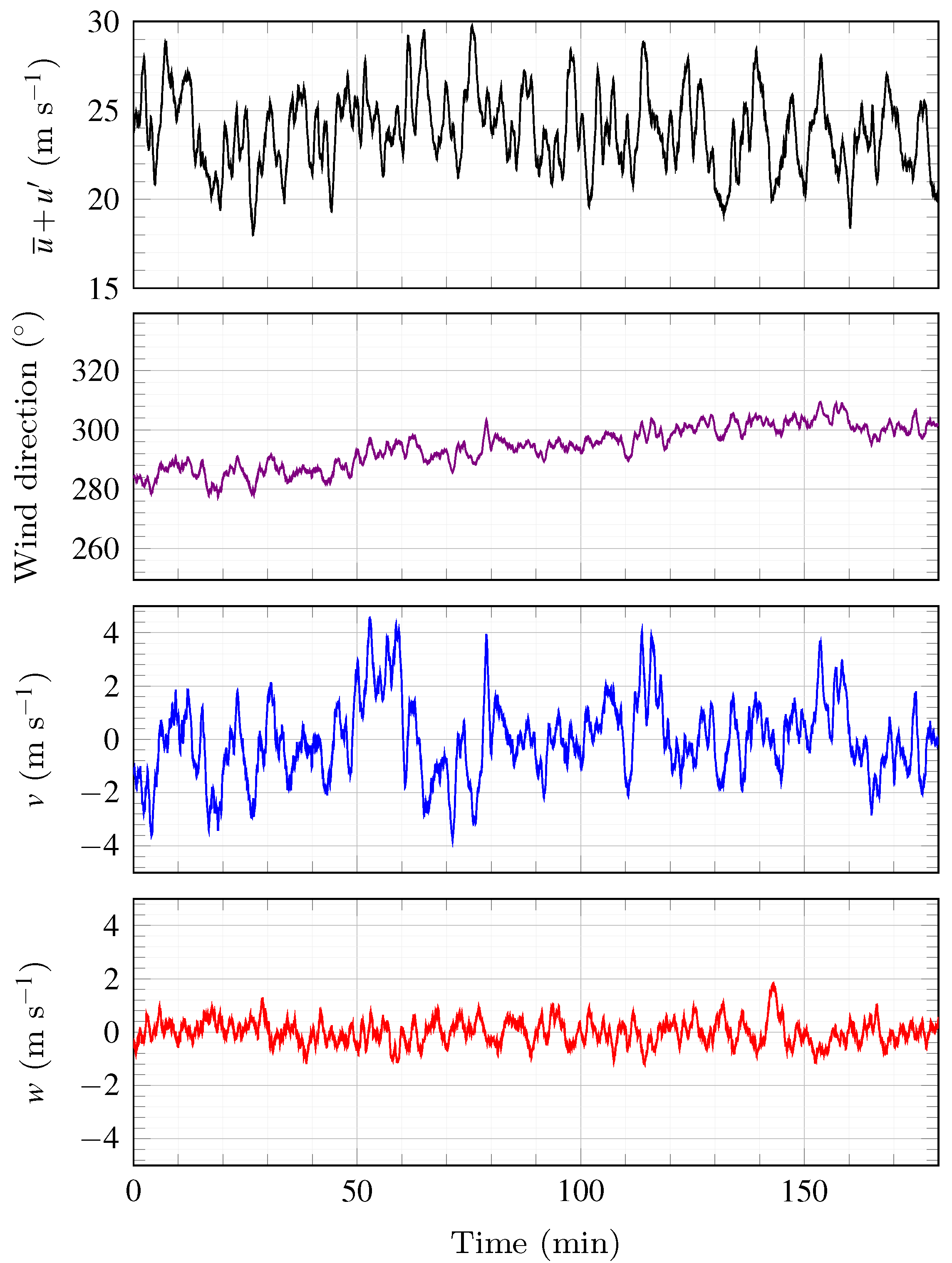
4.1. Flow Characteristics of Wind Storm Aina (2017)

The Bjørnafjord is a 5-km wide and 500-m deep fjord connecting some of the largest export regions of south-western Norway. To strengthen the economy of this area, the new E39 Coastal Highway Route [24] plans to replace the ferries crossing the Bjørnafjord with a 5-km long bridge. The adopted design concept is a floating pontoon bridge, the dimensions of which make it highly sensitive to environmental loading, especially wind turbulence. The homogeneity of the mean and turbulence flow characteristics is a topic of ongoing research in the Bjørnafjord. This fjord is rather flat and open to the sea, such that spatial variations of the flow characteristics remain smooth [76]. This allows for the application of the proposed wind field simulation algorithm. Nevertheless, the southern part of the bridge joining the sea and land will require a dedicated study. Indeed, this part will comprise a long-span cable-stayed bridge in the vicinity of a hill, where turbulence is unusually high and the flow is non-horizontal.
The crossing location is in an open fjord characterized by islands and hills (Figure 2). Therefore, the flow is likely to be skewed along the deck, with a yaw angle up to 45°. Also, the horizontal curvature of the future bridge deck implies that the yaw angle will vary along the bridge span. This motivates the adequate modelling of yawed turbulent flow conditions. Furthermore, the assumption of frozen turbulence may no longer be applicable for the range of frequencies associated with the dynamic motion of such a long bridge.
Since 2015, four 50-m met-masts have been deployed in the Bjørnafjord. Among them, the mast MW1 (Figure 2) was installed 23 m above sea level, on the west side of the fjord, on a small island with low vegetation. It was instrumented with three Gill WindMaster Pro 3-axis 3D sonic anemometers, mounted on 4-m long booms oriented with an angle of −2° from North. Two of the anemometers were located at 49 m above ground but 8 m apart from each other. The third anemometer was 33 m above ground. The masts, supported by guyed wires, have a tubular structure with a diameter of ca. 25 c m to minimize flow distortion. The anemometers recorded the three velocity components at a sampling frequency of 10 Hz but the sonic temperature was not available. The influence of the local topography on the flow characteristics recorded on the mast MW1 under moderate wind conditions is given in Cheynet et al. [76].
Generally, northerly or southerly wind directions prevail along the Norwegian coast. However, a westerly wind was recorded on the second day of storm Aina, which hit the southwestern coast of Norway on 7th and 8th December 2017 [77]. On that day, from 2:00 a.m. to 5:00 a.m., three hours of stationary records with a mean wind speed of 24 m / s at 49 m above ground were recorded on MW1 (Figure 3). The velocity data did not show any clear trend and the mean wind direction increased by only 20° from 2:00 a.m. to 5:00 a.m. The flow was thus fairly stationary because the storm was moving toward the coast instead of along it. The dataset collected that day combines strong wind speed, stationary fluctuations and a duration of at least three hours. Therefore, it is a highly valuable record for the design of the Bjørnafjord bridge.
During storm Aina, two of the three sonic anemometers on MW1 displayed a higher-than-usual measurement noise in the high-frequency range, partly due to aliasing resulting from the use of a 10-Hz sampling frequency without an adequate anti-aliasing filter. In general, a value of 25 Hz is recommended [78]. An additional source of noise may be probe-induced flow distortion due to the geometry of the transducer. Although high-frequency anemometer noise has a limited impact on the study of the root-coherence, it can affect the estimation of the normalized one-point velocity spectra. In particular, this noise can challenge the identification of the inertial subrange. For this reason, the one-point turbulence spectra were studied using one of the two anemometers located 49 m above ground, that was least affected by aliasing and/or flow distortion.
The 3-h event displayed in Figure 3 was characterized by a mean wind direction of 293°, an angle of attack (AoA) of 2.3° and a mean wind speed of 24 m / s . The turbulence characteristics were studied after removing the linear trend in the time series. Using the double rotation technique, the flow was studied in a coordinate system where the vertical mean wind speed is zero. The one-point velocity spectra and cross-spectra were estimated using Welch’s algorithm [79] with a Hamming window, six segments of 30 min and 50% overlapping. Further smoothing was applied by bin averaging the spectral estimates on logarithmically-spaced bins. The root-coherence was also estimated using Welch’s algorithm but with segments of 90 s and 50% overlapping.
The estimated turbulence intensities are summarized in Table 1. In this table, the friction velocity was computed as by Weber [37]. An identical friction velocity was found using the method by Klipp [80], indicating that the double rotation technique is here appropriate. This comparison also suggests that the flow is not substantially affected by lateral shear stress, which can become important in mountainous terrain [81]. The integral flow characteristics identified during this event are consistent with those observed in uniform terrain with moderate roughness length. However, these values differ from those reported in Cheynet et al. [76], collected in May 2016 for a wind direction between 320° and 340°, which were more representative of flow in complex topography. Table 2 summarizes the skewness μ i and kurtosis estimates κ i ( i = u , v , w ). Although the distribution of the w component is slightly skewed toward negative values, the third and fourth-order statistical moments indicate fairly Gaussian fluctuations. Velocity records from the anemometer located 33 m above ground provided similar skewness and kurtosis values as reported in Table 2. Therefore, the turbulence generation scheme described in Section 3 is applicable for the case at hand.

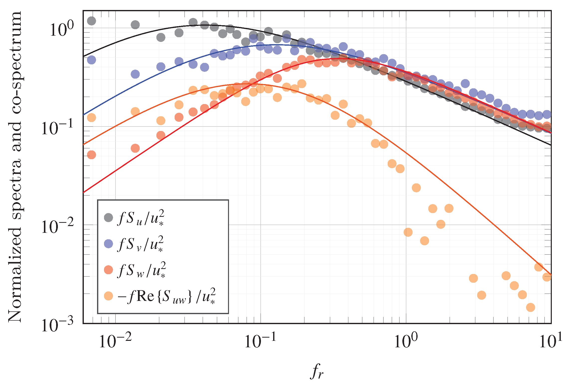
4.2. One-Point Velocity Spectra

Figure 4 shows an excellent agreement between the estimated and fitted power spectral density (PSDs). The least-square fit procedure was applied using Equations (1)–(3) and (7). To better capture the low-frequency fluctuations, only frequencies under 1 Hz were selected. Table 3 shows the values of the coefficients a u , a v and a w (Equations (1)–(3) and (7)) identified for storm Aina. It should be noted that a u = 118 and a w = 3.6 are close to the values found by Kaimal and Finnigan [78] and Busch and Panofsky [82], respectively. Even though the terrain is hilly, the good agreement between fitted and estimated PSDs indicates that, in the present study, surface layer scaling seems to be applicable at a height of 49 m above ground. The friction velocity can be computed based on the covariance term u w ¯ only or by combining u w ¯ and v w ¯ . For the event selected, u w ¯ contributes to more than 95% of the friction velocity. Therefore, the term v w ¯ and the associated cross-spectrum are disregarded hereinafter.
Some discrepancies are visible between the fitted and estimated co-spectrum Re S u w . The cross-spectrum is forced to follow the 7 / 3 slope in the inertial subrange, whereas the estimated co-spectrum does not follow it at f r > 1 . The imaginary part of the cross-spectrum, denoted Im S u w , reflects the blocking by the ground [74] and is not negligible in the present case, which may partly explain these discrepancies. An in-depth study of Im S u w may be valuable for an improved design on slender low-rise structures, such as future floating pontoon bridges, but is out of the scope of the present work.

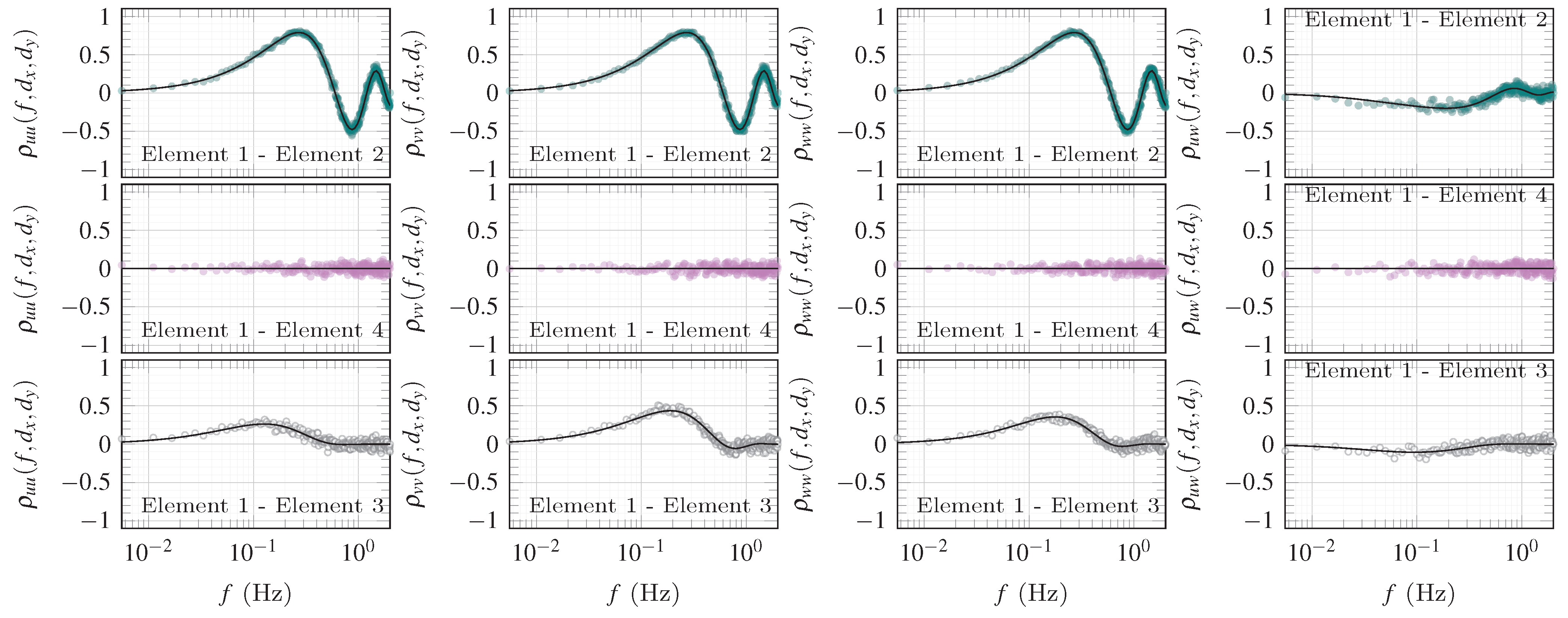
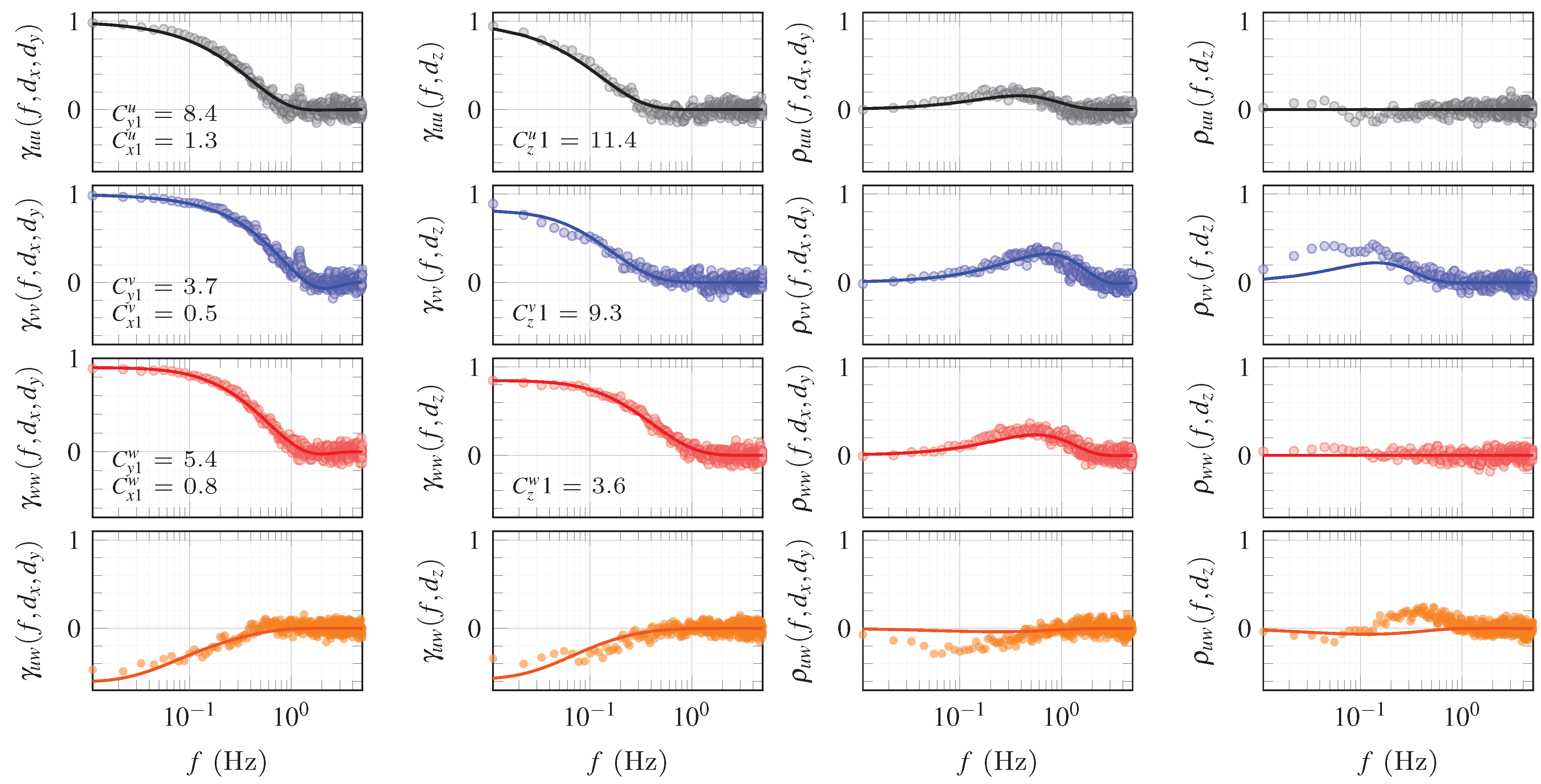
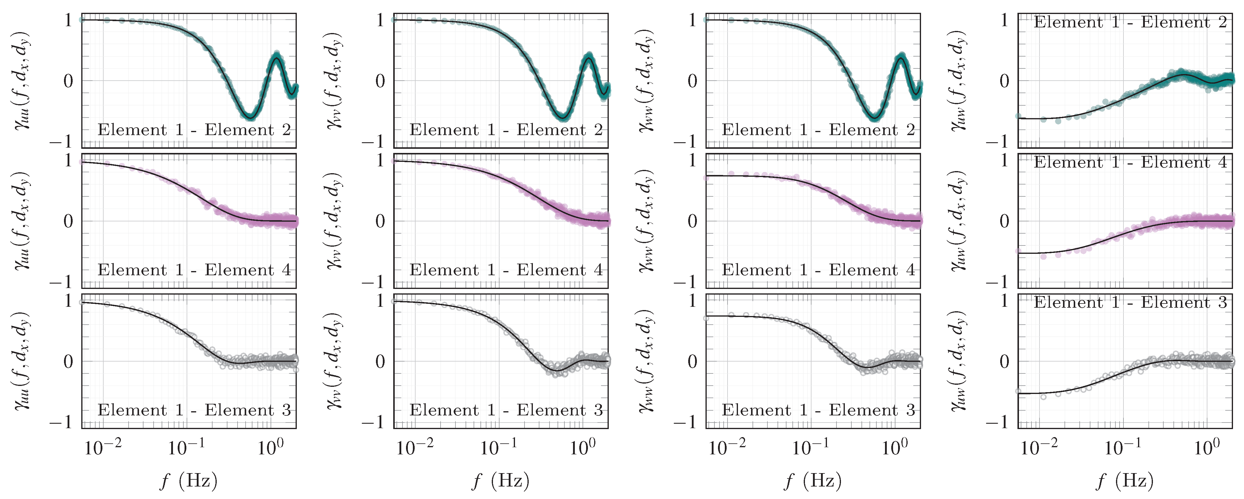
4.3. Coherence Estimates

The co-coherence and quad-coherence estimates obtained using the record collected from 2:00 a.m. to 5:00 a.m. on 8 December 2017 are displayed in Figure 5. They are superposed to the fitted functions γ i i (Equation (32)) and ρ i i (Equation (33)). The vertical root-coherence was studied using the sensors located on the same side of the mast and their horizontal separation was thus zero. Similarly, the horizontal root-coherence was studied using only the sensors at the top of the masts, which were both at 49 m above ground. It should be noted that only frequencies up to 1 Hz were considered for the least-square fit of Equations (32) and (33) since the co-coherence is close to zero at higher frequencies.
Table 4 displays the decay coefficients obtained by least-square fit of Equation (32). For lateral separations, the coefficients are slightly smaller than observed by Kristensen and Jensen [9] on the Sotra bridge, located north of the Bjørnafjord. The parameter c y 1 w is, however, relatively close to the value estimated in the Lysefjord [36]. For vertical separations, the decay coefficients are similar to those estimated above the sea [83], suggesting that the flow incorporates combined characteristics from both offshore and hilly environments. Overall, the identified decay coefficients are within the range of values found by Midjiyawa et al. [84] from multiple masts in three other Norwegian fjords. The along-wind decay coefficients c x 1 j ( j = u , v , w ) are equal to 1, which is also within the range of values derived from the data recorded in the Bjørnafjord with long-range Doppler Wind lidar instruments [22]. A value c x 1 j 1 suggests that Taylor’s hypothesis of frozen turbulence is suitable, at least for the largest eddies. In reality, as soon as c x 1 j > 0 , there exists a range of eddies that cannot be considered frozen any longer and this range increases with the along-wind separation. Finally, it should be noted that the possible dependency of the Davenport decay coefficients on the separation distance (e.g., [58,59]), cannot be explored in the present study because the separation distances are less than 20 m .
Figure 5 shows that the quad-coherence of the u and w component is nearly zero for vertical separations, contrary to the v component. This result supports thus the recommendation provided by ESDU [19]. The solid line used to approximate ρ v v ( f , d z ) is computed using the eddy slope value described in Equation (30), which shows that the low-frequency range is only partly portrayed by the empirical model described in Bowen et al. [59]. On the other hand, the eddy slope has no visible influence on γ v v ( f , d z ) . A more in-depth investigation is required to establish the relevance of the eddy slope when modelling the dynamic wind loading.
The mean yaw angle is here defined with respect to the horizontal line connecting the two sonic anemometers. On 8 December 2017 from 2:00 a.m. to 5:00 a.m., the mean yaw angle was ca. 31° but the co-coherence did not display strongly negative values. To better illustrate the modelling of the negative co-coherence by Equation (32), another sample from storm Aina is selected in Figure 6. In this figure, the record on 8 December 2017, from 20:00 to 23:00 was associated with a stationary mean wind speed and mean wind direction as well as a mean yaw angle of 69°. The sample was, however, less Gaussian and more turbulent than the first sample selected with I u 0.20 as the wind was flowing above rough terrain. Nevertheless, the estimated decay coefficients show only minor differences between the two data samples. The large yaw angle leads to a co-coherence estimate with values as low as −0.6 for the vertical velocity component. The good agreement between the estimated and modelled quad-coherence indicates also that Equation (33) is appropriate for modelling purposes. Finally, Figure 6 shows that the eddy slope is also fairly well captured by Equation (30) for the quad-coherence but not necessarily for the co-coherence, where the eddy slope is not clearly distinguishable.

5. Discussion and Conclusions

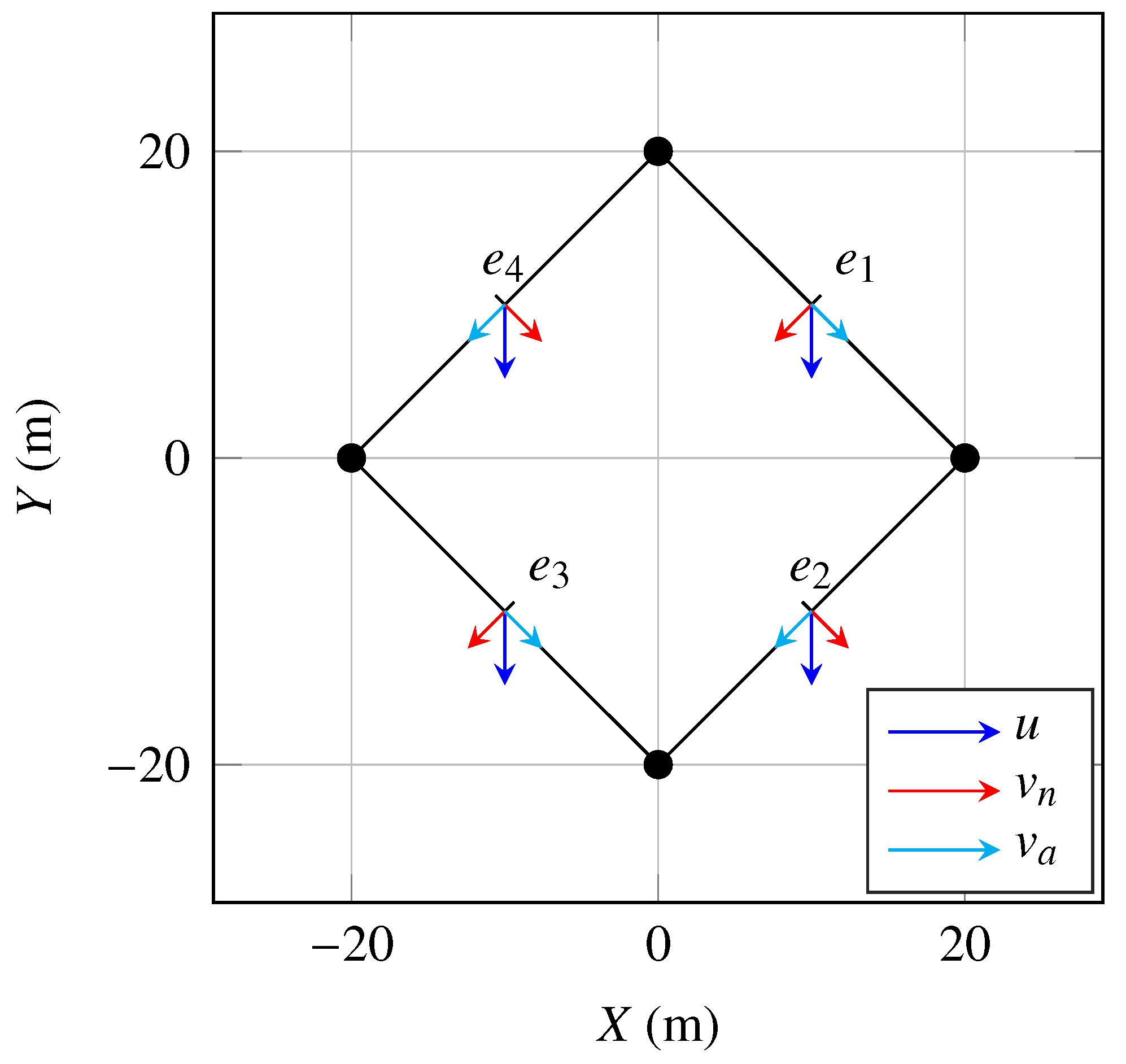
5.1. Skewed Turbulence Generation on a Diamond Geometry

To illustrate the performances of the turbulence generator, ten realizations of a wind field with the same statistical characteristics as for storm Aina are computed. Their statistical properties are estimated for each time series and ensemble-averaged to reduce the random error. The flow field is computed in the middle of the elements of a diamond geometry (Figure 7), denoted e 1 , e 2 , e 3 and e 4 , which has the advantage of including both along-wind and cross-wind separations. The diamond geometry is located in a horizontal plane and does not intend to represent a real structure. Instead, it is used to demonstrate that the turbulent field is properly generated for both along-wind and cross-wind distances. The wind field is generated with a sampling frequency of 4 Hz and 2 14 data points, leading to time series with a duration of ca. 1 h . The reference mean wind speed is set as 24 m / s at a reference height of 49 m above ground with a roughness length z 0 of 0.05   m which is within the range of values found in fjord-like topographies [36,85]. In the following example, the time series are generated at the same height, so there is no need to prescribe a mean wind speed profile. The target velocity spectra are computed based on Equations (1)–(3) and (7) with the parameters estimated in Table 3. Similarly, the target co-coherence model is from Equation (13) with the parameters estimated in Table 4.
In Figure 7, the axes X and Y correspond to the longitude and latitude of the vertices, such that the ( X , Y ) plane is horizontal. The line joining e 1 and e 2 is aligned with the wind direction. Therefore, the along-wind and cross-wind distance between e 2 and e 1 are d x = 20   m and d y = 0   m , respectively. On the other hand, the line joining e 1 and e 4 is perpendicular to the flow, such that d x = 0   m and d y = 20   m . Finally, the line joining e 1 and e 3 combines both cross-wind and along-wind separations, with d x = 20   m and d y = 20   m . Figure 8 displays the time series of the u velocity component on e 1 and e 2 . The normalized cross-correlation function R u ( e 1 , e 2 ) in the bottom panel of Figure 8 reaches its maximum near 0.80   s , which correspond to the advection time between e 1 and e 2 . The largest value of R u ( e 1 , e 2 ) is below 1, which underlines the loss of correlation in the along-wind direction due to the along-wind root-coherence introduced to relax Taylor’s hypothesis of frozen turbulence.
The co-coherence estimates between the different elements are shown as a scatter plot in Figure 9. In this figure, the solid lines correspond to Equation (32) for the co-coherence and to Equation (17) for the cross-coherence. We remind that Equation (17) is only used here for comparison with the simulated cross-coherence, which was numerically implemented using Equation (25). The excellent agreement between target and estimated co-coherence values indicates that the method adopted to generate a yawed flow field with a lower-than-unity co-coherence in the along-wind direction is appropriate. The one-point velocity spectra and co-spectra (Figure 10) show also that the LDL decomposition can be used to model the negative correlation between the u and w components.
The introduction of a time lag in the time series is also reflected by the imaginary part of the root-coherence, which becomes different from zero as soon as d x 0 . In Figure 11, the estimated quad-coherence compares well with the expected one ρ i i . Note that the quad-coherence between the centre of elements 1 and 4 is zero because the local value of the yaw angle is zero. A recent paper by Nybø et al. [86] suggested studying the impact of different quad-coherence formulations on the turbulent load. Following Equation (33), the quad-coherence can be directly derived from the root-coherence combined with the phase lag for longitudinal separations and/or vertical separations. Note that for the case at hand, the quad-coherence did not reflect the phase lag for vertical separations because the elements of the diamond geometry used to compute the flow field were located at the same height above ground.

5.2. Conclusions

The present paper introduces an algorithm to generate a three-variate four-dimensional correlated stationary Gaussian wind field which accounts for non-zero yaw angles and relaxes Taylor’s hypothesis of frozen turbulence. This approach is suitable to model the wind load on slender structures, such as future super-long span bridges crossing Norwegian fjords, which can span from one to five-kilometre distances.
For a structure located mainly in the atmospheric surface layer, the flow field is modelled using surface layer scaling. Turbulence is here governed by the roughness length, the reference wind speed at a reference height, and the one-point and two-point auto- and cross-spectral densities of the velocity fluctuations. Due to the non-zero values of the single-point cross-spectrum for the along-wind and vertical turbulence components, the spectral matrix is not necessarily positive definite. Therefore, the traditional Cholesky decomposition is replaced with the more general LDL factorization. To model non-frozen turbulence, a 3D root-coherence function that accounts for longitudinal separations in addition to the lateral and vertical ones was used.
To illustrate the relevancy of the turbulence parameters selected, measurement data from three 3D sonic anemometers mounted on a meteorological mast on the west coast of Norway were used. The full-scale records were taken from storm Aina (2017), which was characterized by a 3-h mean wind speed of 24 m / s at 49 m above ground. The exceptionally long duration and stationarity of the records allowed an in-depth characterization of the spectral characteristics of turbulence.
The capability of the algorithm to simulate skewed flow conditions is illustrated for a diamond geometry. The time lag was modelled using a complex exponential in the frequency space, which is reflected by the co-coherence and quad-coherence estimates. Although the quad-coherence may not directly participate in the linearised wind load calculation in the frequency domain, it is required for time-domain simulations.
For a 5-km floating pontoon bridge, the proximity of the deck to the sea surface means that appropriate root-coherence and one-point power spectral densities should be used in the wind load modelling. This information could be provided by the algorithm presented herein.

Author Contributions

Conceptualization, E.C.; methodology, E.C., N.D.; software, E.C.; validation, E.C., N.D.; formal analysis, E.C.; investigation, E.C., N.D., J.B.J., J.S. and J.W.; resources, J.W.; data curation, E.C.; writing—original draft preparation, E.C.; writing—review and editing, All co-authors; visualization, E.C. All authors have read and agreed to the published version of the manuscript.

Funding

This research received no external funding.

Data Availability Statement

The algorithm to generate the skewed turbulence field with the relaxation of Taylor’s hypothesis of frozen turbulence is written in Matlab and is available under a BSD-3-Clause open source license (https://doi.org/10.5281/zenodo.7075723 (accessed on 16 September 2022)).

Conflicts of Interest

The authors declare no conflict of interest.

References

  1. Xie, J.; Tanaka, H.; Wardlaw, R.; Savage, M. Buffeting analysis of long span bridges to turbulent wind with yaw angle. J. Wind Eng. Ind. Aerodyn. 1991, 37, 65–77. [Google Scholar] [CrossRef]
  2. Xu, Y.L.; Zhu, L. Buffeting response of long-span cable-supported bridges under skew winds. Part II: Case study. J. Sound Vib. 2005, 281, 675–697. [Google Scholar] [CrossRef]
  3. Diana, G.; Falco, M.; Bruni, S.; Cigada, A.; Larose, G.L.; Darnsgaard, A.; Collina, A. Comparisons between wind tunnel tests on a full aeroelastic model of the proposed bridge over Stretto di Messina and numerical results. J. Wind Eng. Ind. Aerodyn. 1995, 54, 101–113. [Google Scholar] [CrossRef]
  4. Zhu, L.; Wang, M.; Wang, D.; Guo, Z.; Cao, F. Flutter and buffeting performances of Third Nanjing Bridge over Yangtze River under yaw wind via aeroelastic model test. J. Wind Eng. Ind. Aerodyn. 2007, 95, 1579–1606. [Google Scholar] [CrossRef]
  5. Zhu, L.; Xu, Y.L.; Zhang, F.; Xiang, H. Tsing Ma bridge deck under skew winds—Part I: Aerodynamic coefficients. J. Wind Eng. Ind. Aerodyn. 2002, 90, 781–805. [Google Scholar] [CrossRef]
  6. Diana, G.; Resta, F.; Zasso, A.; Belloli, M.; Rocchi, D. Effects of the yaw angle on the aerodynamic behaviour of the Messina multi-box girder deck section. Wind Struct. 2004, 7, 41–54. [Google Scholar] [CrossRef]
  7. Davenport, A.G. The response of slender, line-like structures to a gusty wind. In Proceedings of the Institution of Civil Engineers; Thomas Telford-ICE Virtual Library: London, UK, 1962; Volume 23, pp. 389–408. [Google Scholar]
  8. Larose, G.L. The spatial distribution of unsteady loading due to gusts on bridge decks. J. Wind Eng. Ind. Aerodyn. 2003, 91, 1431–1443. [Google Scholar] [CrossRef]
  9. Kristensen, L.; Jensen, N. Lateral coherence in isotropic turbulence and in the natural wind. Bound.-Layer Meteorol. 1979, 17, 353–373. [Google Scholar] [CrossRef]
  10. Solari, G.; Piccardo, G. Probabilistic 3-D turbulence modeling for gust buffeting of structures. Probabilistic Eng. Mech. 2001, 16, 73–86. [Google Scholar] [CrossRef]
  11. Strømmen, E.; Hjorth-Hansen, E. Static and dynamic section model tests of the proposed Hardanger fjord suspension bridge. In Proceedings of the Bridges into the 21st Century, Hong Kong, China, 2–5 October 1995; p. 8. [Google Scholar]
  12. Zhu, L.; Xu, Y.L. Buffeting response of long-span cable-supported bridges under skew winds. Part I: Theory. J. Sound Vib. 2005, 281, 647–673. [Google Scholar] [CrossRef]
  13. Jafari, M.; Sarkar, P.P. Wind-induced response characteristics of a yawed and inclined cable in ABL wind: Experimental-and numerical-model based study. Eng. Struct. 2020, 214, 110681. [Google Scholar] [CrossRef]
  14. Raeesi, A.; Cheng, S.; Ting, D.S.K. Application of a three-dimensional aeroelastic model to study the wind-induced response of bridge stay cables in unsteady wind conditions. J. Sound Vib. 2016, 375, 217–236. [Google Scholar] [CrossRef]
  15. Robertson, A.N.; Shaler, K.; Sethuraman, L.; Jonkman, J. Sensitivity analysis of the effect of wind characteristics and turbine properties on wind turbine loads. Wind Energy Sci. 2019, 4, 479–513. [Google Scholar] [CrossRef]
  16. Sanchez Gomez, M.; Lundquist, J.K. The effect of wind direction shear on turbine performance in a wind farm in central Iowa. Wind Energy Sci. 2020, 5, 125–139. [Google Scholar] [CrossRef]
  17. Liu, Z.; Zheng, C.; Wu, Y.; Flay, R.G.; Zhang, K. Investigation on the effects of twisted wind flow on the wind loads on a square section megatall building. J. Wind Eng. Ind. Aerodyn. 2019, 191, 127–142. [Google Scholar] [CrossRef]
  18. Feng, C.; Gu, M.; Zheng, D. Numerical simulation of wind effects on super high-rise buildings considering wind veering with height based on CFD. J. Fluids Struct. 2019, 91, 102715. [Google Scholar] [CrossRef]
  19. ESDU. ESDU 86010, Characteristics of Atmospheric Turbulence Near the Ground. Part III: Variations in Space and Time for Strong Winds (Neutral Atmosphere); IHS Inc.: London, UK, 2002. [Google Scholar]
  20. Taylor, G.I. The spectrum of turbulence. Proc. R. Soc. Lond. Ser.-Math. Phys. Sci. 1938, 164, 476–490. [Google Scholar] [CrossRef]
  21. Simley, E.; Pao, L.Y. A longitudinal spatial coherence model for wind evolution based on large-eddy simulation. In Proceedings of the 2015 American Control Conference (ACC), Chicago, IL, USA, 1–3 July 2015; pp. 3708–3714. [Google Scholar]
  22. Cheynet, E.; Jakobsen, J.; Snæbjörnsson, J.; Mann, J.; Courtney, M.; Lea, G.; Svardal, B. Measurements of Surface-Layer Turbulence in a Wide Norwegian Fjord Using Synchronized Long-Range Doppler Wind Lidars. Remote Sens. 2017, 9, 977. [Google Scholar] [CrossRef]
  23. Shinozuka, M.; Deodatis, G. Simulation of Stochastic Processes by Spectral Representation. Appl. Mech. Rev. 1991, 44, 191. [Google Scholar] [CrossRef]
  24. Eidem, M.E. Overview of floating bridge projects in Norway. In Proceedings of the International Conference on Offshore Mechanics and Arctic Engineering, American Society of Mechanical Engineers, Trondheim, Norway, 25–30 June 2017; p. 8. [Google Scholar]
  25. da Costa, B.M.; Wang, J.; Jakobsen, J.B.; øiseth, O.A.; þór Snæbjörnsson, J. Bridge buffeting by skew winds: A quasi-steady case study. J. Wind Eng. Ind. Aerodyn. 2022, 227, 105068. [Google Scholar] [CrossRef]
  26. Zerva, A.; Zervas, V. Spatial variation of seismic ground motions: An overview. Appl. Mech. Rev. 2002, 55, 271–297. [Google Scholar] [CrossRef]
  27. Zhang, D.Y.; Liu, W.; Xie, W.C.; Pandey, M.D. Modeling of spatially correlated, site-reflected, and nonstationary ground motions compatible with response spectrum. Soil Dyn. Earthq. Eng. 2013, 55, 21–32. [Google Scholar] [CrossRef]
  28. Monin, A.S.; Obukhov, A.M. Basic laws of turbulent mixing in the surface layer of the atmosphere. Contrib. Geophys. Inst. Acad. Sci. USSR 1954, 151, e187. [Google Scholar]
  29. Kaimal, J.; Wyngaard, J.; Izumi, Y.; Coté, O. Spectral characteristics of surface-layer turbulence. Q. J. R. Meteorol. Soc. 1972, 98, 563–589. [Google Scholar] [CrossRef]
  30. Panofsky, H.; Dutton, J. Atmospheric Turbulence: Models and Methods for Engineering Applications; Wiley-Interscience: New York, NY, USA, 1984. [Google Scholar]
  31. Barthelmie, R. The effects of atmospheric stability on coastal wind climates. Meteorol. Appl. A J. Forecast. Pract. Appl. Train. Tech. Model. 1999, 6, 39–47. [Google Scholar] [CrossRef]
  32. Olesen, H.R.; Larsen, S.E.; Højstrup, J. Modelling velocity spectra in the lower part of the planetary boundary layer. Bound.-Layer Meteorol. 1984, 29, 285–312. [Google Scholar] [CrossRef]
  33. Tieleman, H.W. Universality of velocity spectra. J. Wind Eng. Ind. Aerodyn. 1995, 56, 55–69. [Google Scholar] [CrossRef]
  34. Kolmogorov, A.N. The local structure of turbulence in incompressible viscous fluid for very large Reynolds numbers. Dokl. Akad. Nauk SSSR 1941, 30, 299–303. [Google Scholar]
  35. Peña, A.; Dellwik, E.; Mann, J. A method to assess the accuracy of sonic anemometer measurements. Atmos. Meas. Tech. Discuss. 2018, 2018, 1–23. [Google Scholar] [CrossRef]
  36. Cheynet, E.; Jakobsen, J.B.; Snæbjörnsson, J. Flow distortion recorded by sonic anemometers on a long-span bridge: Towards a better modelling of the dynamic wind load in full-scale. J. Sound Vib. 2019, 450, 214–230. [Google Scholar] [CrossRef]
  37. Weber, R.O. Remarks on the definition and estimation of friction velocity. -Bound.-Layer Meteorol. 1999, 93, 197–209. [Google Scholar] [CrossRef]
  38. Haugen, D.; Kaimal, J.; Bradley, E. An experimental study of Reynolds stress and heat flux in the atmospheric surface layer. Q. J. R. Meteorol. Soc. 1971, 97, 168–180. [Google Scholar] [CrossRef]
  39. Charnock, H. Wind stress on a water surface. Q. J. R. Meteorol. Soc. 1955, 81, 639–640. [Google Scholar] [CrossRef]
  40. Högström, U. Review of some basic characteristics of the atmospheric surface layer. Bound.-Layer Meteorol. 1996, 78, 215–246. [Google Scholar] [CrossRef]
  41. Burlando, M.; Carassale, L.; Georgieva, E.; Ratto, C.F.; Solari, G. A simple and efficient procedure for the numerical simulation of wind fields in complex terrain. Bound.-Layer Meteorol. 2007, 125, 417–439. [Google Scholar] [CrossRef]
  42. Dörenkämper, M.; Olsen, B.T.; Witha, B.; Hahmann, A.N.; Davis, N.N.; Barcons, J.; Ezber, Y.; García-Bustamante, E.; González-Rouco, J.F.; Navarro, J.; et al. The making of the new european wind atlas—Part 2: Production and evaluation. Geosci. Model Dev. 2020, 13, 5079–5102. [Google Scholar] [CrossRef]
  43. Haakenstad, H.; Breivik, ø.; Furevik, B.R.; Reistad, M.; Bohlinger, P.; Aarnes, O.J. NORA3: A Nonhydrostatic High-Resolution Hindcast of the North Sea, the Norwegian Sea, and the Barents Sea. J. Appl. Meteorol. Climatol. 2021, 60, 1443–1464. [Google Scholar] [CrossRef]
  44. Øiseth, O.; Rönnquist, A.; Sigbjörnsson, R. Effects of co-spectral densities of atmospheric turbulence on the dynamic response of cable-supported bridges: A case study. J. Wind Eng. Ind. Aerodyn. 2013, 116, 83–93. [Google Scholar] [CrossRef]
  45. ESDU. ESDU 85020, Characteristics of Atmospheric Turbulence Near the Ground. Part II: Single Point Data for Strong Winds (Neutral Atmosphere); IHS Inc.: London, UK, 2001. [Google Scholar]
  46. EN 1991-1-4; Eurocode 1: Actions on Structures–Part1-4: General Actions-Wind Actions. Comité Européen de Normalization (CEN): Brussels, Belgium, 2005.
  47. Norwegian Public Road Administration. N400 Handbook for Bridge Design; Directorate of Public Roads: Oslo, Norway, 2015.
  48. Hill, R. Corrections to Taylor’s frozen turbulence approximation. Atmos. Res. 1996, 40, 153–175. [Google Scholar] [CrossRef]
  49. Monin, A. Turbulence in the atmospheric boundary layer. Phys. Fluids 1967, 10, S31–S37. [Google Scholar] [CrossRef]
  50. Higgins, C.W.; Froidevaux, M.; Simeonov, V.; Vercauteren, N.; Barry, C.; Parlange, M.B. The effect of scale on the applicability of Taylor’s frozen turbulence hypothesis in the atmospheric boundary layer. Bound.-Layer Meteorol. 2012, 143, 379–391. [Google Scholar] [CrossRef]
  51. Tong, C. Taylor’s hypothesis and two-point coherence measurements. Bound.-Layer Meteorol. 1996, 81, 399–410. [Google Scholar] [CrossRef]
  52. Ropelewski, C.F.; Tennekes, H.; Panofsky, H. Horizontal coherence of wind fluctuations. Bound.-Layer Meteorol. 1973, 5, 353–363. [Google Scholar] [CrossRef]
  53. Burghelea, T.; Segre, E.; Steinberg, V. Validity of the Taylor hypothesis in a random spatially smooth flow. Phys. Fluids 2005, 17, 103101. [Google Scholar] [CrossRef]
  54. Sjöholm, M.; Mikkelsen, T.; Kristensen, L.; Mann, J.; Kirkegaard, P. Spectral analysis of wind turbulence measured by a Doppler LIDAR for velocity fine structure and coherence studies. In Proceedings of the 15th International Symposium for the Advancement of Boundary Layer Remote Sensing, Paris, France, 28–30 June 2010; p. 5. [Google Scholar]
  55. Davoust, S.; von Terzi, D. Analysis of wind coherence in the longitudinal direction using turbine mounted lidar. In Proceedings of the Journal of Physics: Conference Series; IOP Publishing: Bristol, UK, 2016; Volume 753, p. 072005. [Google Scholar]
  56. Debnath, M.; Brugger, P.; Simley, E.; Doubrawa, P.; Hamilton, N.; Scholbrock, A.; Jager, D.; Murphy, M.; Roadman, J.; Lundquist, J.K.; et al. Longitudinal coherence and short-term wind speed prediction based on a nacelle-mounted Doppler lidar. In Proceedings of the Journal of Physics: Conference Series; IOP Publishing: Bristol, UK, 2020; Volume 1618, p. 032051. [Google Scholar]
  57. Chen, Y.; Schlipf, D.; Cheng, P.W. Parameterization of Wind Evolution using Lidar. Wind Energy Sci. Discuss. 2020, 6, 61–91. [Google Scholar] [CrossRef]
  58. Kristensen, L.; Panofsky, H.A.; Smith, S.D. Lateral coherence of longitudinal wind components in strong winds. Bound.-Layer Meteorol. 1981, 21, 199–205. [Google Scholar] [CrossRef]
  59. Bowen, A.J.; Flay, R.G.; Panofsky, H.A. Vertical coherence and phase delay between wind components in strong winds below 20 m. Bound.-Layer Meteorol. 1983, 26, 313–324. [Google Scholar] [CrossRef]
  60. Davenport, A.G. The spectrum of horizontal gustiness near the ground in high winds. Q. J. R. Meteorol. Soc. 1961, 87, 194–211. [Google Scholar] [CrossRef]
  61. Pielke, R.; Panofsky, H. Turbulence characteristics along several towers. Bound.-Layer Meteorol. 1970, 1, 115–130. [Google Scholar] [CrossRef]
  62. Hjorth-Hansen, E.; Jakobsen, A.; Strømmen, E. Wind buffeting of a rectangular box girder bridge. J. Wind Eng. Ind. Aerodyn. 1992, 42, 1215–1226. [Google Scholar] [CrossRef]
  63. Minh, N.N.; Miyata, T.; Yamada, H.; Sanada, Y. Numerical simulation of wind turbulence and buffeting analysis of long-span bridges. J. Wind Eng. Ind. Aerodyn. 1999, 83, 301–315. [Google Scholar] [CrossRef]
  64. Shinozuka, M.; Jan, C.M. Digital simulation of random processes and its applications. J. Sound Vib. 1972, 25, 111–128. [Google Scholar] [CrossRef]
  65. Veers, P.S. Three-Dimensional Wind Simulation; Technical report; Sandia National Labs.: Albuquerque, NM, USA, 1988. [Google Scholar]
  66. Shinozuka, M.; Deodatis, G. Simulation of Multi-Dimensional Gaussian Stochastic Fields by Spectral Representation. Appl. Mech. Rev. 1996, 49, 29. [Google Scholar] [CrossRef]
  67. Jonkman, B.J.; Buhl, M.L., Jr. TurbSim User’s Guide; Technical Report; National Renewable Energy Lab. (NREL): Golden, CO, USA, 2006. [Google Scholar]
  68. Mann, J. Wind field simulation. Probabilistic Eng. Mech. 1998, 13, 269–282. [Google Scholar] [CrossRef]
  69. Benowitz, B.A.; Deodatis, G. Simulation of wind velocities on long span structures: A novel stochastic wave based model. J. Wind Eng. Ind. Aerodyn. 2015, 147, 154–163. [Google Scholar] [CrossRef]
  70. de Maré, M.; Mann, J. On the space-time structure of sheared turbulence. Bound.-Layer Meteorol. 2016, 160, 453–474. [Google Scholar] [CrossRef]
  71. Hémon, P.; Santi, F. Simulation of a spatially correlated turbulent velocity field using biorthogonal decomposition. J. Wind Eng. Ind. Aerodyn. 2007, 95, 21–29. [Google Scholar] [CrossRef]
  72. Ashcraft, C.; Grimes, R.G.; Lewis, J.G. Accurate symmetric indefinite linear equation solvers. SIAM J. Matrix Anal. Appl. 1998, 20, 513–561. [Google Scholar] [CrossRef]
  73. Duff, I.S. MA57-a New Code for the Solution of Sparse Symmetric Definite Systems; Technical Report; CM-P00045911; CLRC: Oxford, UK, 2002. [Google Scholar]
  74. Mann, J. The spatial structure of neutral atmospheric surface-layer turbulence. J. Fluid Mech. 1994, 273, 141–168. [Google Scholar] [CrossRef]
  75. Chougule, A.; Mann, J.; Kelly, M.; Sun, J.; Lenschow, D.; Patton, E. Vertical cross-spectral phases in neutral atmospheric flow. J. Turbul. 2012, 13, 36. [Google Scholar] [CrossRef]
  76. Cheynet, E.; Jakobsen, J.; Snæbjörnsson, J.; Ágústsson, H.; Harstveit, K. Complementary use of wind lidars and land-based met-masts for wind measurements in a wide fjord. JPhCS 2018, 1104, 012028. [Google Scholar] [CrossRef]
  77. Rommetveit, A. Ekstremværet Aina Kan Bli Farlig. 2017. Available online: https://www.yr.no/artikkel/ekstremvaeret-aina-kan-bli-farlig-1.13814154 (accessed on 7 December 2017).
  78. Kaimal, J.C.; Finnigan, J.J. Atmospheric Boundary Layer Flows: Their Structure and Measurement; Oxford University Press: Oxford, UK, 1994. [Google Scholar]
  79. Welch, P. The use of fast Fourier transform for the estimation of power spectra: A method based on time averaging over short, modified periodograms. IEEE Trans. Audio Electroacoust. 1967, 15, 70–73. [Google Scholar] [CrossRef] [Green Version]
  80. Klipp, C. Turbulent friction velocity calculated from the Reynolds stress Tensor. J. Atmos. Sci. 2018, 75, 1029–1043. [Google Scholar] [CrossRef]
  81. Midjiyawa, Z.; Cheynet, E.; Reuder, J.; Ágústsson, H.; Kvamsdal, T. Potential and challenges of wind measurements using met-masts in complex topography for bridge design: Part I–Integral flow characteristics. J. Wind Eng. Ind. Aerodyn. 2021, 211, 104584. [Google Scholar] [CrossRef]
  82. Busch, N.E.; Panofsky, H.A. Recent spectra of atmospheric turbulence. Q. J. R. Meteorol. Soc. 1968, 94, 132–148. [Google Scholar] [CrossRef]
  83. Cheynet, E.; Jakobsen, J.B.; Reuder, J. Velocity spectra and coherence estimates in the marine atmospheric boundary layer. Bound.-Layer Meteorol. 2018, 169, 429–460. [Google Scholar] [CrossRef]
  84. Midjiyawa, Z.; Cheynet, E.; Reuder, J.; Ágústsson, H.; Kvamsdal, T. Potential and challenges of wind measurements using met-masts in complex topography for bridge design: Part II—Spectral flow characteristics. J. Wind Eng. Ind. Aerodyn. 2021, 211, 104585. [Google Scholar] [CrossRef]
  85. Harstveit, K. Full scale measurements of gust factors and turbulence intensity, and their relations in hilly terrain. J. Wind Eng. Ind. Aerodyn. 1996, 61, 195–205. [Google Scholar] [CrossRef]
  86. Nybø, A.; Nielsen, F.G.; Reuder, J.; Churchfield, M.J.; Godvik, M. Evaluation of different wind fields for the investigation of the dynamic response of offshore wind turbines. Wind Energy 2020, 23, 1810–1830. [Google Scholar] [CrossRef]
Figure 1. Time delay Δ t ( y s 1 , y s 2 ) between points located at p 1 and p 2 for a incoming frozen turbulent flow with a yaw angle β and a mean wind speed u ¯ . The x and y axis are the horizontal axes and z is the positive vertical axis.
Applsci 12 09537 g001
Figure 2. Topography of the Bjørnafjord sketching the future bridge crossing and the mast MW1 used in the analysis of the velocity data.
Applsci 12 09537 g002
Figure 3. One-minute moving average time series corresponding to storm Aina (December 2017) from 2:00 a.m. to 5:00 a.m. on 8 December 2017 using one of two anemometers mounted 49 m above ground on MW1.
Applsci 12 09537 g003
Figure 4. Estimated (scatter) and fitted (solid lines) one-point auto- and cross-power spectral estimates at z = 49   m above ground from 2:00 a.m. to 5:00 a.m. on 8 December 2017.
Applsci 12 09537 g004
Figure 5. Co-coherence and quad-coherence of the three velocity components estimated for a wind direction of 293°, u ¯ = 24   m / s at z = 49   m above ground and a yaw angle of 31° ( d x = 4.1   m , d y = 6.9   m , and d z = 16   m ). The data were recorded on 8 December 2017 from 02:00 to 05:00. The solid lines correspond to the best fit of Equation (32) for the co-coherence and Equation (33) for the quad-coherence.
Applsci 12 09537 g005
Figure 6. Co-coherence and quad-coherence of the three velocity components estimated for a wind direction of 331°, u ¯ = 18   m / s at z = 49   m above ground and a yaw angle of 69° ( d x = 7.5   m , d y = 2.9   m , and d z = 16   m ). The data were recorded on 8 December 2017 from 20:00 to 23:00. The solid lines correspond to the best fit of Equation (32) for the co-coherence and Equation (33) for the quad-coherence.
Applsci 12 09537 g006
Figure 7. Diamond geometry used to validate the skewed turbulence generation algorithm. The flow is simulated in the middle of elements 1 to 4 with a northern wind direction. For each structural element e i ( i = 1 , 2 , 3 , 4 ), the axial and normal velocity components are denoted v a and v n , respectively.
Applsci 12 09537 g007
Figure 8. First five minutes of the time series of the fluctuating along-wind velocity components generated on e 1 and e 2 (top panel) and associated cross-correlation function (bottom panel).
Applsci 12 09537 g008
Figure 9. Target co-coherence (solid lines) and estimated one (markers) between elements 1 and 2 (top panels), elements 1 and 4 (middle panels) and elements 1 and 3 (bottom panels) of the diamond geometry.
Applsci 12 09537 g009
Figure 10. Target and computed power spectral densities estimates on e 1 .
Applsci 12 09537 g010
Figure 11. Target quad-coherence (solid lines) and estimated one (markers) between elements 1 and 2 (top panels), elements 1 and 4 (middle panels) and elements 1 and 3 (bottom panels) of the diamond geometry.
Applsci 12 09537 g011
Table 1. Second-order integral turbulence characteristics recorded at 49 m above ground on MW1 (Bjørnafjord) on 8 December 2017 from from 2:00 a.m. to 5:00 a.m.
Characteristics I u I v I w u * (m s 1 ) σ u / u * σ v / u * σ w / u * I v / I u I w / I u
0.140.110.081.362.431.961.340.810.55
Table 2. Third and fourth-order integral turbulence characteristics recorded at 49 m above ground on MW1 (Bjørnafjord) on 8 December 2017 from from 2:00 a.m. to 5:00 a.m. For i = u , v , w , the skewness estimates are denoted μ i whereas the kurtosis estimates are named κ i .
Characteristics μ u μ v μ w κ u κ v κ q
0.050.070.152.73.23.3
Table 3. Spectral parameters from Equations (1)–(3) and (7) estimated using wind data recorded from 2:00 a.m. to 5:00 a.m. on 8 December 2017 on MW1.
Coefficients a u a v a w a uw b uw
Values118243.6129
Table 4. Decay coefficients estimated on 8 December 2017 from 2:00 to 5:00 on MW1. These coefficients are eastimated by least-square fit of Equation (13).
Component i c x 1 j c y 1 j c y 2 j c z 1 j c z 2 j
u180.01110.03
v140.0190.30
w150.3640.24
Publisher’s Note: MDPI stays neutral with regard to jurisdictional claims in published maps and institutional affiliations.

