Abstract
In recent years, scheduling optimization has been utilized in production systems. To construct a suitable mathematical model of a production scheduling problem, modeling techniques that can automatically select an appropriate objective function from historical data are necessary. This paper presents two methods to estimate weighting factors of the objective function in the scheduling problem from historical data, given the information of operation time and setup costs. We propose a machine learning-based method, and an inverse optimization-based method using the input/output data of the scheduling problems when the weighting factors of the objective function are unknown. These two methods are applied to a multi-objective parallel machine scheduling problem and a real-world chemical batch plant scheduling problem. The results of the estimation accuracy evaluation show that the proposed methods for estimating the weighting factors of the objective function are effective.
1. Introduction
The optimization model for scheduling problems consists of boundary conditions, decision variables, constraints, and objective functions. In practice, it is difficult to adapt to changes in the selection of objective functions and weighting factors for multi-objective optimization problems when constructing an optimization model for production scheduling problems. Data-driven optimization is one of the decision-making methods based on quantitative data [1]. In the data-driven approach, the actions are determined after the data is collected, stored, and analyzed. This allows past information to be incorporated into future decision-making factors. The data-driven optimization approach has been widely used in various fields such as supply chain, transportation systems, and healthcare [2,3,4], and it is required for modeling complex production scheduling problems.
Scheduling optimization has become an important issue in recent years. Many companies have interests to upgrade their industrial facilities to meet the Industry 4.0 paradigm. At the same time, they are required to optimally manage their production systems. In recent years, real-world scheduling problems have become complicated due to complex constraints and objective functions. Scheduling algorithms using the concepts of linear optimization and batch operation scheduling [5] and nonlinear optimization theory and batch scheduling [6] have been proposed and applied to a chemical industrial site. Methods for integrating multiple time scales to increase process efficiency have also been studied [7]. The application of game theoretical approaches to job scheduling has also been studied in the distributed scheduling methods. An autonomous decentralized scheduling [8,9], non-cooperative game approach for scheduling [10], and evolutionary game theory approach [11] have been addressed. Recently, restaurant scheduling with resource allocation [12] has also been proposed. These approaches have been successfully applied to the job scheduling problems. It is also required to help decision-makers to build an optimization model from historical and real-time data for efficiency and flexibility of production systems. In online scheduling, algorithms have been proposed which take real-time data into account [13]. Scheduling problems with multiple objectives require mathematical models that reflect human operators’ preferences based on multiple optimization criteria [14]. However, it is difficult to set the appropriate weighting factors for the objective function in a multi-objective scheduling problem [15]. Scheduling is a complex task that is often determined manually or by simulation. As a result, suboptimal solutions are derived [16]. If weighting factors that do not reflect the operator’s intention are set, an undesired schedule will be generated. In that situation, human operators must manually fine-tune the schedule when the circumstances surrounding the production environment change. Thus, the weighting factors need to be modified iteratively in the multi-objective scheduling problem [17,18]. The estimation of the weighting factors is required because the human operators can efficiently obtain the schedule originally desired. For example, when we automatically determine the weighting factors of the objective function, the input/output data is effectively used to quantify the evaluation criteria of the production schedules that had been already in operation. As a result, the weighting factor of the daily schedule result can be quantitatively analyzed.
In this paper, we propose a machine learning method and an inverse optimization method to estimate weighting factors of the objective function for model identification of production scheduling problems. In machine learning, features for weighting factor estimation are selected using a wrapper method. In recent years, machine learning has grown rapidly with the increase in data and the development of computers performance. On the other hand, inverse optimization is used to estimate the internal structure based on the input/output data of the target and to optimize from input to output based on it, and various studies have been conducted [19,20]. In the machine learning method, we attempt to extract effective features to improve the estimation accuracy. Additionally, the weighting factor is estimated by the inverse optimization to compare the performance with that of machine learning. The difference in the estimation results for the small-scale and large-scale problems is studied. The proposed method is applied to a parallel machine scheduling problem for a chemical batch plant. From the result of computational experiments, it was confirmed that using feature selection approach can improve the accuracy of weighting factor estimation in machine learning for the parallel machine scheduling problems.
The contributions of this paper are as follows. We propose a model identification method for multi-objective scheduling problems based on historical scheduling data. We propose the wrapper method for feature selection to select effective features for weighting factor estimation. We apply our proposed method to realistic data for a scheduling problem of a chemical batch plant.
This paper is organized as follows. First, we discuss related work for weighting factor estimation in Section 2. We then explain the problem definition of scheduling problems and weighting factor estimation. The machine learning method is described in Section 3, and the inverse optimization method is proposed in Section 4. In Section 5, we perform numerical experiments on the proposed method. We conclude and discuss future work in Section 6.
2. Literature Review
Analytic Hierarchy Process (AHP) is one of the traditional decision-making methods for estimating weighting factors for multi-criteria decision-making [21]. Evaluation is performed by pairwise comparison for multiple evaluation criteria and alternatives. The pairwise comparison determines the importance of evaluation criteria and alternatives. It is effective in rationalizing complicated decision-making. Since it is a simple method, it is used in various situations. For example, the AHP model is used to evaluate the components of a machining center so that the manufacturer can purchase the most suitable machining center [22]. However, when there are so many evaluation criteria and alternative options, it is too complicated to set appropriate pairwise comparisons for multiple evaluation criteria.
In general, the methods for solving multi-objective optimization problems are classified into the following three methods depending on the situation in which the decision-maker involves the process [23].
- A priori methods: The decision maker specifies the preferred objective function before executing the solution process.
- Interactive methods: Phases of interaction between decision-makers and the solution process are iteratively conducted.
- Posteriori or generation methods: After the solutions are generated by the weighting method or -constraint method, the decision-maker selects the preferred solution.
In this study, the a priori method is used to solve the scheduling problems. However, the aim of this study is to estimate the weighting factor of a scheduling problem instead of solving it.
A previous study on the identification of the objective function was conducted to read the operator’s intentions from the input/output data of a scheduling problem [24]. In the single-objective scheduling problem, the objective function used was estimated from historical data in the literature. This was conducted for only one objective function. However, in an actual factory, there are multiple objective functions to be optimized in many cases. The methods for solving multi-objective optimization problems have been extensively studied in the literature. A decomposition-based evolutionary multi-objective optimization algorithm is used, which transforms a multi-objective optimization problem into several single objective optimization problems and optimizes them simultaneously [25]. For the three-objective scheduling problem, a three-phase decision-making method is constructed, and finally, a data envelopment analysis technique is applied to determine the preferred schedule [26]. Dynamic scheduling is proposed to solve the optimization problem of selecting the next job for each schedule [27]. In multi-objective flow shop scheduling, optimization algorithms are used which consider changes in material requirements, inventory control, and delivery dates [23]. To solve the multi-objective scheduling problems, there is a method of setting a weighting factor for each objective function to create a single objective function. To reflect the operator’s intentions from the past schedule, it is necessary to estimate the weighting factors of the objective function.
Previous studies on weighting factor estimation are described. The inverse problem using linear programming was used to estimate the weighting factors after the range of weighting factor that derives a preferred solution is derived when a person in the field makes decisions [18]. However, this method has not been applied to the actual scheduling problem in the literature. In reference [28], a method for estimating the weighting factors from past scheduling data has been proposed for small-scale scheduling problems. However, the scale of production processes in the conventional study is not so large because the exact optimal solutions are used to find the weighting factors by using commercial solvers. It becomes intractable to utilize exact algorithms for large scale problems. Therefore, various approximate solution methods have been proposed for solving large-scale scheduling problems [29]. The simulated annealing method was used to minimize the total loading time of the container in the scheduling problem of the two-transtainer system [30]. For flexible job shop scheduling problems, an effective algorithm that combines a genetic algorithm and tabu search has been proposed [31]. In reference [32], weighting factors were estimated for large-scale scheduling problems. A simulated annealing method was used to solve the scheduling problem and a near-optimal solution was derived. However, in machine learning, the features to be selected for estimating the weighting factors were combined manually in the literature. It becomes more difficult as the number of features increases. Efficient feature selection methods that can improve estimation accuracy are required for machine learning methods.
We address the model identification of the multi-objective scheduling problem and apply the wrapper method as a feature selection method for estimating weighting factors in this paper.
3. Problem Description
This section describes the multi-objective scheduling problem used in this study and the weighting factor estimation problem.
3.1. Definition of Multi-Objective Parallel Machine Scheduling Problem
In this section, we describe the multi-objective unrelated parallel machine scheduling problem. The objectives of this problem are to determine the assignment of jobs to some machines and the job processing order. This problem is subject to three constraints. The unrelated parallel machine scheduling problem has no specific restrictions on the processing time of each job. Additionally, the processing speed of each machine is different. It is more general than related parallel machine scheduling problems that the processing speed of each machine is the same.
The following three constraints are given:
- There is no idle time set for each machine.
- One machine can only handle one job at a time.
- Each job cannot be interrupted during processing. No preemption is allowed.
In the scheduling problem, the obtained schedules are different depending on the objective function.
3.2. Weighting Factor Estimation Problem from Historical Data
Noise and unnecessary information in the actual historical data interfere with the estimation of the weighting factors of the objective function. Therefore, we use the scheduling results (starting time of operations, production sequence of operations) and the parameters of the scheduling problem as input/output data. The possibility of using these input/output data for system identification to estimate the model is considered, but we refrain from using them because the relationship between the schedule and the weighting factors is difficult to ascertain. It is still difficult to estimate the weighting factors from the solution of the multi-objective scheduling problem because most of the scheduling problem is NP (non-deterministic polynomial-time) hard, and there is no one-to-one relation between the solution of the scheduling problem and the correct weighting factors of the objective function. Another challenge is how to find effective features from the input/output data. The problem can be used in many realistic situations due to the following reasons.
- When the plant is operated by human experts, they will set appropriate weighting factors in daily scheduling. The derived weighting factors can be used to understand the expert knowledge of human operators.
- The solutions of the scheduling system can be used to set appropriate weighting factors of the objective function when an automated scheduling system is equipped in a real factory.
The outline of the weighting factor estimation is shown in Figure 1. In this study, the near-optimal solutions of the scheduling problem are regarded as the actual data for estimating the weighting factors. We assume a parallel machine production scheduling problem. The processing time, job delivery time, and setup cost are given as input data. The output data includes job assignments, processing order, and objective function values. The weighting factor is estimated using these input/output data. Machine learning methods and inverse optimization are used to estimate the weighting factors. The model is evaluated by the mean squared error (MSE) between the estimated weighting factor and the true weighting factor. MSE is expressed by Equation (1), where is the estimated weighting factor, is the true weighting factor, and is the number of data.
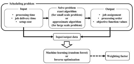
Figure 1.
Outline of the weighting factor estimation.
4. Weighting Factor Estimation Method from Scheduling Results
Weighting factor estimation method using historical scheduling data is described. Machine learning and inverse optimization for weighting factor estimation are proposed.
4.1. Machine Learning
In this section, weighting factor estimation using machine learning is described. The outline of machine learning method is shown in Figure 2.
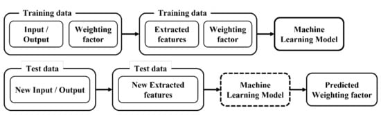
Figure 2.
Outline of machine learning method.
First, we prepare 100 problem examples of the scheduling problem. Information such as delivery time, processing time, and setup cost is given as input parameters to the scheduling problem. A set of weighting factors is given to this input to solve the scheduling problem and obtain the output. The output contains the job processing order, job assignment, and each objective function value. The input data and weighting factors corresponding to the output results are known. For small-scale problems, an exact solution is obtained, and for large-scale problems, an approximate solution is obtained by simulated annealing. The obtained input/output data is divided 8 to 2 into training and test data. Then, the input/output data are converted into features. Then, machine learning models are constructed by training data. Finally, machine learning is used to estimate the test data. The machine learning method that we used in this study is random forest [33]. Random forest is one of the supervised learning methods and it constructs a model with higher generalization performance by using multiple decision trees. A regression random forest is used to output the estimated weighting factor as a continuous value. The decision tree is formed by multiple explanatory variables. It is undesirable to use the input/output data of a scheduling problem as is in machine learning. To construct a highly accurate model with random forest, it is necessary to extract features that strongly represent the relationship between the weighting factors and the schedule. In this study, we use features for the explanatory variable. Conversely, including features that have no relationship may generate noise during learning, increase computation time, and decrease prediction accuracy. We will explain how to generate features used in random forests in Section 4.2.
4.2. Feature Extraction
This section describes the feature extraction methods used in machine learning. Features that are considered effective for estimating weighting factors are extracted. The features vary depending on the objective function used and the scale of the problem.
4.2.1. Small Scale Problems with 2 Objectives Optimization Problems
First, the features used for the small-scale problems with 2 objectives are explained [28]. In the 2 objectives case, the maximum completion time and the sum of setup costs are used as objective functions. The objective function of the scheduling problem is expressed by Equation (2).
where represents the weighting factor of objective function , represents completion time of job at machine , represents 1 when job is processed next to job at machine , 0 otherwise, represents setup cost when switching from job to job . We considered the following features: 1. The values of the maximum completion time, 2. The values of the sum of setup costs, 3. The variance of completion time for each machine, and 4. Spearman’s rank correlation coefficients (). The objective function values are extracted because they are related to the weighting factors. If the objective of the maximum completion time is emphasized, the difference between the completion times between machines is small. Therefore, it is used as a feature of the variation of the completion time expressed by Equation (3).
where represents number of machines, represents maximum completion time of machine , represents mean of completion time of each machine. Figure 3 shows Gantt charts with different weighting factors. The vertical dashed lines represent processing times of 300 and 600. In Figure 3a, the maximum completion time is emphasized, and in Figure 3b, it is not emphasized. In this case, the variance of the maximum completion time is effective.
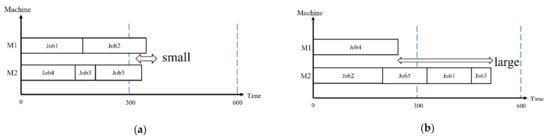
Figure 3.
Gantt charts with different weighting factor: (a) maximum completion time is emphasized; (b) maximum completion time is not emphasized.
represents starting time order of job in ascending order, represents processing time order of job in ascending order. The orders are indexed by an integer value such as 1, 2, 3, …, according to the value of starting time of job . Others are the same. Spearman’s rank correlation coefficient, which represents the correlation between the ranks of the two indicators, is used. Since the maximum completion time is used as the objective function, a rank correlation is generated from the processing sequence of the job and the job processing time order. The obtained rank correlation value is represented by Equation (4). represents number of jobs, is , is .
4.2.2. Large Scale Problems with 2 Objectives Optimization Problems
Then, the features for large-scale problems are proposed. We try to extract effective features when the objective function is different. The sum of delivery delay and the sum of setup costs is used as the objective function. The objective function of the scheduling problem is expressed in Equation (5).
where represent a delay in delivery of job at machine . Since the objective function has changed from small-scale problems, it is necessary to change the features used. Features that are not related to the weighting factor do not contribute to the improvement of estimation accuracy, so it is not preferable to use the same features. We considered the following features: 5. The values of the sum of delivery delay, 2. The values of the sum of setup costs, 6. The variance of delivery time setting for each machine, 7. The sum of completion time of each machine, and 8. Spearman’s rank correlation coefficients (). For the problem of minimizing the sum of delivery delays in the case of one machine, the optimal schedule can be obtained by processing in the order of earliest delivery time. It is effective even in the case of multiple machines. In that case, there is no difference in the delivery date set by each machine. The variance of delivery time setting for each machine is represented by Equation (6).
where represents total delivery time of job processed of machine , represents mean of the delivery time of job processed by each machine. If the sum of delivery delay is minimized, the job needs to be completed in less time. It is considered that the sum of delivery delay and the total completion time are related. The sum of completion time of each machine is represented by Equation (7).
where represents 1 when job is processed at machine , 0 otherwise, represents processing time at job at machine . represents delivery time order of job in ascending order. Since the objective function has changed from the maximum completion time to the sum of delivery delays, a rank correlation is generated from the processing sequence of the job and the job delivery time order. It is represented by Equation (4). is , is .
4.2.3. Small Scale Problems with 3 Objectives Optimization Problems
Next, we consider a scheduling problem with three objective functions. Three of the following five objective functions are combined. The objective functions used are as follows.
- maximum completion time + sum of weighted delivery delay + sum of setup costs
- sum of weighted completion time + maximum weighted delivery delay + sum of setup costswhere represents weight of job . We considered the following features: 1. The values of the maximum completion time (Case I only), 2. The values of the sum of setup costs, 3. The variance of completion time for each machine, 4. Spearman’s rank correlation coefficients (), 6. The variance of delivery time setting for each machine, 7. The sum of completion time of each machine, 8. Spearman’s rank correlation coefficients (), 9. The values of the sum of weighted delivery delay (Case I only), 10. The values of sum of weighted completion time (Case II only), 11. The values of maximum weighted delivery delay (Case II only), 12. The shortest processing time selectivity, 13. Spearman’s rank correlation coefficients (), 14. Spearman’s rank correlation coefficients (), 15. Spearman’s rank correlation coefficients (), 16. Spearman’s rank correlation coefficients (), and 17. Spearman’s rank correlation coefficients (). Feature 12 indicates the degree to which a job is processed by a machine with a short processing time. The smaller the value, the more jobs are assigned to machines with shorter processing times. The shorter the processing time of a job, the smaller the value of the objective function other than the sum of setup costs. Therefore, there is a relationship between the weighting factor for the objective functions other than the sum of setup costs. The shortest processing time selectivity is expressed by Equation (10).
Features 4, 8, 13~17 are Spearman’s rank correlation coefficients. The rank correlation is generated from the two rankings in parentheses. For the 3-objective case, rank correlations are extracted, including the weights of the jobs. represents order of job in ascending order. represents order of job in ascending order. represents order of job in ascending order. represents order of job in ascending order. Rank correlation coefficients is represented by Equation (4). correspond to the two symbols in parentheses features 4, 8, 13~17, respectively.
4.3. Feature Selection
In this section, we describe how to combine the features extracted in Section 4.2. There are three main goals of feature selection. The three main goals are to improve prediction performance, to improve computational efficiency, and to understand the relationship between the results and the features. There are three main feature selection methods commonly used: filter methods, wrapper methods, and embedded methods [34]. The filter method statistically ranks each feature and decides whether to use it for prediction. It is computationally efficient, but because it confirms at features one by one, the combined effect of features cannot be checked. The wrapper method determines which features to select by adding (or deleting) features that will increase (or decrease) the accuracy the most from the already selected features. Compared to the filter method, the wrapper method improves accuracy, but the computational cost increases as the number of features increases. The embedded method determines the features to be selected based on the importance of each feature during model prediction. It is a well-balanced method between the filter and wrapper methods. In this study, the wrapper method is used. There are two types of wrapper methods: sequential forward selection (SFS), which adds features, and sequential backward selection (SBS), which removes features. In this study, SFS is used. Outline of wrapper feature selection method is shown in Figure 4. The procedure is as follows.
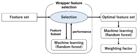
Figure 4.
Outline of wrapper feature selection method.
- Start with an empty set and add the feature that improves accuracy the most to the subset .
- Add the feature that improves accuracy the most when adding features to subset . The MSE is computed when the feature is added.
- If the state of Equation (11) is maintained, go to 2. Otherwise, exit.
is a subset of the selected features and is a subset of the features when feature is added. is constant, is the number of selected features.
Many sets of features are extracted as described in Section 4.2 and the weighting factors corresponding to each problem are prepared. Features and the corresponding weighting factors are divided into training data for training in a random forest, and test data for examining the accuracy of the machine learning model. When dividing, stratified sampling is performed so that the weighting factors are not biased. When dividing a node in random forest, the data is divided by the feature that minimizes the impure of the node. The MSE is used as an impure index when dividing a node. The division is performed so that this impure index is the smallest. After constructing a learning model from the training data, new test data that does not include the weighting factor is inputted into the model, and the weighting factor is estimated. In the regression type random forest method, the weighting factor is outputted as a continuous value. The model is evaluated by the MSE between the estimated weighting factor and the true weighting factor.
4.4. Inverse Optimization
Inverse optimization is finding the input that generates the output, given the output of an optimization problem [35]. When applied to the weighting factor estimation problem, the output is the scheduling results, and the input is the weighting factors. We will describe how to estimate the weighting factors using the inverse optimization method. First, many schedule data, solved by changing the weighting factor from 0.1 to 0.9 by 0.1, are prepared. The scheduling problem is solved by giving an initial weighting factor. The weighting factors are updated to reduce the error between the resulting output and the desired output. The scheduling problem is solved again with the updated weighting factor. By repeating this, the weighting factors are estimated. The model is evaluated by the MSE between the estimated weighting factor and the true weighting factor. It is applied to both small- and large-scale problems. The outline of the inverse optimization algorithm is shown in Algorithm 1 [36].
| Algorithm 1: Inverse optimization |
The input data are the initialized weighting factors. The weighting factor is initialized on line 1. On the 5th line, the scheduling problem is solved after the initial value of the weighting factor is set. The optimal solutions are obtained at line 5. Exact solutions are obtained by a commercial solver for small-scale problems, and the approximate solutions are obtained for large-scale problems. In lines 6 and 7, the gradient of the weighting factor is computed, and the loss function is used for the gradient. Solutions with known weighting factor and optimal solutions are used to calculate the gradient. The loss function is calculated by solving some problems. The number of problems on the 4th line is set to 10. After that, the weighting factor is updated on line 9. When updating, the update width is divided by the number of problems and multiplied by the learning rate . The iteration is executed with the maximum number of iterations , and the weighting factor output on the 11th line is the result of the weighting estimation.
5. Computational Experiments
The procedure of the numerical experiment is explained in this section. First, we generate the input data. Then, we solve the scheduling problem using the exact solution and approximate solution. We create a dataset from the input data and the obtained output data and apply it to each model. Finally, we evaluate the accuracy of the model by the MSE of the estimated weighting factor with the true weighting factor. MSE is expressed by Equation (1). For machine learning, the dataset was divided into 5 parts and 5-fold cross validations were performed.
For small-scale problems, the number of machines is 3 and the number of jobs is 7. For large-scale problems, the number of machines is 5 and the number of jobs is 50. The parameters of the scheduling problem are given randomly in the range of Table 1 and Table 2. Table 1 shows small-scale problems and Table 2 shows large-scale problems. A total of 100 scheduling problems were prepared for each case. The weighting factor was changed by 0.1 from 0.1 to 0.9. For the small-scale problems, CPLEX solver was used to obtain an exact solution, and for the large-scale problems, simulated annealing was used to obtain an approximate solution. In machine learning, 900 data sets are used for the 2 objectives and 3600 data sets are used for the 3 objectives. MSE is obtained from these numbers of data. In the random forest, the number of decision trees is set to 100 and the tree depth to 5. in SFS is set to 0.001. In inverse optimization, the maximum number of iterations is 15, the learning rate is 0.5, the number of problem instances is 10.

Table 1.
Parameter of input data in small-scale problems.
Table 2.
Parameter of input data in large-scale problems.
5.1. Effectiveness of Features in Machine Learning
First, it is applied to small-scale problems. Objective function is the maximum completion time and the sum of setup costs. The case where only the objective function values were used as features was compared with the case where features were selected by SFS from the features extracted in Section 4.2.1. Table 3 shows the features selected by SFS in the order in which they were selected. Table 4 shows the MSE of the estimation results.
Table 3.
List of features selected by SFS for small-scale problems for 2 objectives.
Table 4.
MSE results of machine learning to small-scale problems for 2 objectives.
In SFS, all the extracted features were selected. As a result, the accuracy is higher than that obtained by learning only the objective function values in a random forest. The order in which the features were selected is noteworthy: the objective function values were selected first. This was closely related to the change in the weighting factor, since they were included in the equation of the scheduling problem.
Then, the target problem is extended to a large scale. The objective function is the sum of the delivery delay and the sum of the setup costs. The case where only the objective function values were used as features was compared with the case where features were selected by SFS from the features extracted in Section 4.2.2. Table 5 shows the features selected by SFS in the order in which they were selected. Table 6 shows the MSE of the estimation results.
Table 5.
List of features selected by SFS for large-scale problems for 2 objectives.
Table 6.
MSE results of machine learning for large-scale problems for 2 objectives.
In SFS, all extracted features were selected even for large-scale problems. Compared to the estimation of objective function values only, the estimation with features selected by SFS was more accurate. However, the improvement in accuracy was not as great as for small-scale problems. As the problem size increases, a small change in the weighting factors causes the objective function values to change. This was effective during machine learning. For the large-scale problem, an approximate solution method was used to solve the scheduling problem. These results suggest that the objective function values obtained by the approximate solution method changes more easily than objective function values obtained by exact solution method.
Then, estimation was performed for 3 objectives in small-scale problems. Experiments were performed on two different objective functions. Each objective function is shown in Section 4.2.3. The case where only the objective function values were used as features was compared with the case where features were selected by SFS from the features extracted in Section 4.2.2. Table 7 shows the features selected by SFS in the order in which they were selected. Table 8 shows the MSE of the estimation results.
Table 7.
List of features selected by SFS small-scale problems for 3 objectives.
Table 8.
MSE results of machine learning to small-scale problems for 3 objectives.
First, we consider case I. In SFS, only two features were selected. However, it is more accurate than the estimation with 3 objective function values. In the case of valid features, the estimation is possible even with a small number of features. The features that are valid in case 1 are the sum of setup costs and the variance of completion time for each machine.
Next, we consider case II. Five features were selected by SFS. The accuracy is better than the estimation using only the objective function values. As in case 1, the sum of setup costs and the variance of completion time for each machine are selected. The rank correlation coefficients between job processing time and processing order were also effective in the estimation. There is no significant difference in estimation accuracy between case I and case II.
5.2. Comparison of Each Case in Machine Learning
A comparison between small-scale and large-scale problems is discussed. Table 9 shows a comparison between small-scale and large-scale problems in machine learning.
Table 9.
MSE results of machine learning.
First, for the 2 objectives, we compare small-scale and large-scale problems. Large-scale problems are more accurate. In small-scale problems, the objective function value often does not change even if the weighting factors change. The fact that the value does not change is the cause of the lack of accuracy in machine learning. Next, we compare 2 objectives and 3 objectives for small-scale problems. 3 objectives were more accurate. As the number of objectives increased, the objective function values changed more easily. This worked well in machine learning.
5.3. Comparison of Each Case in Inverse Optimization
The inverse optimization is applied to problems of each case. Figure 5 shows the weighting factor estimation for the small-scale problem (2 objectives). The initial value of the weighting factor is set to (, ) = (0.7, 0.3). The target weighting factor is (, ) = (0.2, 0.8). The target weighting factor is reached after the 10th iteration.
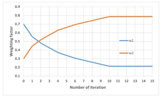
Figure 5.
The result of estimation (initial value is (, ) = (0.7, 0.3) target value is (, ) = (0.2, 0.8)).
Table 10 shows the estimation error in MSE for each case. First, in the 2-objective case, small-scale and large-scale problems are compared. The accuracy of the large-scale problem was higher than that of the small-scale problem. It is thought that the change in the objective function value has something to do with this. In small-scale problems, the objective function value may not change even if the weighting factors change. In such a case, the estimation is completed before reaching the weighting factors to be estimated. Therefore, it is thought that the estimation accuracy becomes low. Next, the 2-objective and 3-objective cases are compared in the small-scale case. The 2-objective case is more accurate. In the 2-objective case, as the weighting factor increases, the corresponding objective function value decreases. But this is not necessarily the case for the 3-objective case.
Table 10.
MSE result of inverse optimization.
We consider an example of the weighting factor and objective function values for the case I. When the weighting factor is () = (0.2, 0.3, 0.5), the objective function value is (390, 2982, 1241). On the other hand, when the weighting factor is () = (0.5, 0.1, 0.4), the objective function values are (478, 3783, 754). The value of maximum completion time for the first objective function increases as the weighting factor increases. The value of sum of setup costs for the third objective function decreases as the weighting factor decreases. In this case, the weighting factors are not updated correctly.
5.4. Comparison of Machine Learning Method and Inverse Optimization Method
The results of machine learning and inverse optimization are compared. Table 11 shows the comparison between machine learning and inverse optimization for each problem scale. The machine learning value is the one with the better accuracy when the feature is the objective function value, or the feature selected by SFS.
Table 11.
MSE result of each case.
In all cases, inverse optimization is more accurate than machine learning. In the 2-objectives case, inverse optimization is significantly more accurate. In the 2-objectives case, the change in the objective function value varies monotonically with the weighting factors. The gradients of the weighting factors are easy to compute. In the case of the 3-objectives, the gradients of the weighting factors were not calculated properly in some cases.
5.5. Application to Chemical Batch Plants
We apply the proposed methods to a production scheduling problem in a chemical batch plant. In this paper, we use the lubricating oil filling schedule in chemical batch plants. The job contents and constraints will be briefly explained. A total of 34 filling operations are given. The filling amount, the drum to be filled, and the delivery date are shown for each. There are 9 types of drums to fill. The filling speed differs depending on the type. Filling works consist of the following three steps. 1. Cleaning and draining oil from the line, 2. Product edge, and 3. Filling. There are two main time constraints. Filling work start time is 09:05. Break times are 10:30–11:00, 12:00–13:00, and 15:00–15:30. Filling work cannot be done during the above break time. If the type of oil is different from the previous oil during cleaning, cleaning costs (setup costs) are incurred. Two objective functions are used in chemical batch plant scheduling: the sum of delivery delays and the sum of setup costs. The objective function is expressed in Equation (5). The required amount of filling of each oil differs from day to day. An approximate solution method is used for the input/output data. We considered the following features: 5. The values of the sum of delivery delay, 2. The values of the sum of setup costs, and 7. The sum of completion time of each machine. We prepared 270 data sets. Machine learning evaluates the data by performing 5-cross-validation. The case where only the objective function values were used as features was compared with the case where features were selected by SFS from the features extracted in Section 4.2.1. The hyperparameters for machine learning and inverse optimization are the same as in Section 5.
Figure 6 and Figure 7 show the Gantt chart when the weighting factor is and . The gray bar sections on the Gantt chart represent break time. Table 12 shows the features selected by SFS in the order in which they were selected. Table 13 shows the MSE of the estimation results.
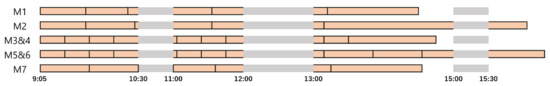
Figure 6.
Weighting factor is (, ) = (0.5, 0.5).
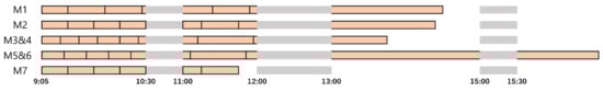
Figure 7.
Weighting factor is (, ) = (0.9, 0.1).
Table 12.
List of features selected by SFS.
Table 13.
MSE results of machine learning and inverse optimization.
Since the number of tanks that can be assigned to a job is predetermined, only seven machines were used in this case. Figure 7 shows that many machines have shorter completion times compared to Figure 6. As a result, the value of the sum of delivery delays is smaller. Table 12 shows that all features are selected. The order in which the features are selected is the same as for the large-scale problem. Since the objective function is the same, the order of effective features is also the same. Furthermore, the MSE is smaller than when only the objective function value is used as features. It was confirmed that feature extraction is effective even when the data is close to real data. In inverse optimization, estimation accuracy was better than machine learning. However, both were less accurate than when the scheduling problem was generated randomly. In the randomly generated problems, setup costs varied slowly. The real data, however, do not vary slowly because the setup cost is predetermined to a certain value due to the nature of the problem. This is the reason why the accuracy of the inverse optimization was lower than that of the randomly generated problems.
5.6. Discussion
SFS was used in feature selection from the extracted features. As a result, in all cases, the accuracy was higher than estimating the weighting factors using only the objective function values. In addition, the selected features were different for each case. We found that even a small number of features can be estimated with good accuracy if they are valid features. The feature of variance of completion time was effective for small-scale problems. Especially in case I, it was judged to be more effective in improving accuracy than the objective function values other than the setup cost sum.
For the large-scale problem, the accuracy was particularly better compared to the other cases. This is because the objective function values are more variable than in the small-scale case. In the inverse optimization, the weighting factors were estimated almost exactly by repeatedly solving the scheduling problem. The approximate solution method was also highly accurate. In addition to the objective function value, the sum of completion time of each machine and the variance of delivery time setting for each machine were found to be effective in machine learning for large-scale problems. However, the improvement in accuracy from estimating only the objective function value was smaller than that for small-scale problems.
Experiments on near-realistic data confirmed the same trend as for randomly generated problems. However, the estimation accuracy was low, partly because there were problems in which the objective function value of the sum of setup costs did not change much.
The following insights obtained from our study are as follows.
- In randomly generated problems, the estimation accuracy of the large-scale problem was higher than that of the small-scale problem because the solution changed continuously in response to the change of the weighting factor.
- In the case of machine learning, the feature of the variance of completion time for each machine was effective for small-scale problems, and the features of the sum of completion time of each machine and the variance of delivery time setting for each machine were effective for large-scale problems.
- When using the input/output data of the same scheduling model, if a solution close to the exact solution is used, the inverse optimization has higher estimation accuracy than machine learning because the gradient was recalculated many times during the estimation process.
6. Conclusions
In this study, we estimated the weighting factors of the objective function in the production scheduling problem from input/output data. The scheduling problem was expanded on a large scale and an approximate solution was applied. Simulated annealing was used as the approximate solution method. Two methods were used to estimate the weighting factors: machine learning and inverse optimization. It was confirmed that feature selection in SFS works effectively and improves estimation accuracy. It also evaluated performance using an inverse optimization method. Future work is to confirm whether the proposed method is effective for other scheduling problems. Extracting valid features other than the objective function value from the scheduling results, when applied to actual data, is also required.
Author Contributions
Conceptualization, H.T., K.A. and T.N.; methodology, H.T., K.A. and T.N.; software, H.T., K.A. and T.N.; validation, H.T. and K.A.; formal analysis, H.T.; investigation, H.T.; resources, T.N.; data curation, K.A.; writing—original draft preparation, H.T., K.A., T.N. and Z.L.; writing—review and editing, H.T., K.A., T.N. and Z.L.; visualization, H.T.; supervision, T.N.; project administration, T.N.; funding acquisition, T.N. All authors have read and agreed to the published version of the manuscript.
Funding
This research was funded by JSPS KAKENHI(B) 22H01714.
Institutional Review Board Statement
Not applicable.
Informed Consent Statement
Not applicable.
Data Availability Statement
Data is contained within the article.
Conflicts of Interest
The authors declare no conflict of interest.
Abbreviations
| AHP | analytic hierarchy process |
| MSE | mean squared error |
| SFS | sequential forward selection |
| SBS | sequential backward selection |
| Symbol | |
| MSE | |
| Number of data | |
| Estimated weighting factor | |
| True weighting factor | |
| Feature extraction | |
| Number of jobs | |
| Number of machines | |
| Weight of objective function f | |
| Weight of job i | |
| Processing time at job at machine | |
| Setup cost when switching from job i to job j | |
| Completion time of job i at machine k | |
| Delay in delivery of job i at machine k | |
| 1 when job j is processed immediately after job i at machine k, 0 otherwise | |
| 1 when job i is processed at machine k, 0 otherwise | |
| Maximum completion time of machine | |
| Mean of completion time of each machine | |
| Total delivery date of job processed of machine | |
| Mean of the delivery date of job processed by each machine | |
| Starting time order of job in ascending order | |
| Weight order of job in ascending order | |
| Processing time order of job in ascending order | |
| Delivery time order of job in ascending order | |
| order of job in ascending order | |
| order of job in ascending order | |
| order of job in ascending order | |
| order of job in ascending order | |
| Variation of the completion time | |
| Spearman’s rank correlation coefficients | |
| Variance of delivery time setting for each machine | |
| Sum of completion time of each machine | |
| Shortest processing time selectivity | |
| Feature selection | |
| Feature | |
| Subset of the selected features | |
| Feature that improves accuracy the most when adding features to subset | |
| Subset of the features when feature is added | |
| Constant expressing the degree of tolerance | |
| Number of selected features | |
| Inverse optimization | |
| Initial weighting factor | |
| Maximum number of iterations | |
| Solutions with known weighting factor | |
| Learning rate | |
| Number of problem instances |
References
- Provost, F.; Fawcett, T. Data Science and its Relationship to Big Data and Data-Driven Decision Making. Big Data 2013, 1, 51–59. [Google Scholar] [CrossRef] [PubMed]
- Kamble, S.S.; Gunasekaran, A.; Gawankar, S.A. Achieving sustainable performance in a data-driven agriculture supply chain: A review for research and applications. Int. J. Prod. Econ. 2020, 219, 179–194. [Google Scholar] [CrossRef]
- Zhang, J.; Wang, K. Data-Driven Intelligent Transportation Systems: A Survey. IEEE Trans. Intell. Transp. Syst. 2011, 12, 1624–1639. [Google Scholar] [CrossRef]
- Whitt, W.; Zhang, X. A data-driven model of an emergency department. Oper. Res. Health Care 2017, 12, 1–15. [Google Scholar] [CrossRef]
- Vaccari, M.; di Capaci, R.B.; Brunazzi, E.; Tognotti, L.; Pierno, P.; Vagheggi, R.; Pannocchia, G. Implementation of an Industry 4.0 system to optimally manage chemical plant operation. IFAC-PapersOnLine 2020, 53, 11545–11550. [Google Scholar] [CrossRef]
- Vaccari, M.; di Capaci, R.B.; Brunazzi, E.; Tognotti, L.; Pierno, P.; Vagheggi, R.; Pannocchia, G. Optimally Managing Chemical Plant Operations: An Example Oriented by Industry 4.0 Paradigms. Ind. Eng. Chem. Res. 2021, 60, 7853–7867. [Google Scholar] [CrossRef]
- Burnak, B.; Pistikopoulos, E.N. Integrated process design, scheduling, and model predictive control of batch processes with closed-loop implementation. AIChE J. 2020, 66, e16981. [Google Scholar] [CrossRef]
- Nishi, T.; Sakata, A.; Hasebe, S.; Hashimoto, I. Autonomous decentralized scheduling system for just-in-time production. Comput. Chem. Eng. 2000, 24, 345–351. [Google Scholar] [CrossRef]
- Nishi, T.; Konishi, M.; Hasebe, S. An autonomous decentralized supply chain planning system for multi-stage production processes. J. Intell. Manuf. 2005, 16, 259–275. [Google Scholar] [CrossRef]
- Zhou, G.; Jiang, P.; Huang, G.Q. A game-theory approach for job scheduling in networked manufacturing. Int. J. Adv. Manuf. Technol. 2009, 41, 972–985. [Google Scholar] [CrossRef]
- Lee, J.W.; Kim, M.K. An Evolutionary Game theory-based optimal scheduling strategy for multiagent distribution network operation considering voltage management. IEEE Access 2022, 10, 50227–50241. [Google Scholar] [CrossRef]
- Taehyeun, P.; Walid, S. Kolkata Paise Restaurant Game for resource allocation in the Internet of Things. In Proceedings of the 2017 51st Asilomar Conference on Signals, Systems, and Computers, Pacific Grove, CA, USA, 29 October–1 November 2017; pp. 1774–1778. [Google Scholar] [CrossRef]
- Venkatachalam, A.; Christos, T.M. State estimation in online batch production scheduling: Concepts, definitions, algorithms and optimization models. Comput. Chem. Eng. 2021, 146, 107209. [Google Scholar] [CrossRef]
- Baker, K.R.; Smith, J.C. A Multiple-Criterion Model for Machine Scheduling. J. Sched. 2003, 6, 7–16. [Google Scholar] [CrossRef]
- Aoki, Y. Multi-Objective Optimization Method. Oper. Res. 1978, 23, 511–516. [Google Scholar]
- Georgiadis, G.R.; Elekidis, A.R.; Georgiadis, M.C. Optimization-based scheduling for the process industries: From theory to real-life industrial applications. Processes 2019, 7, 438. [Google Scholar] [CrossRef]
- Watanabe, S.; Hiroyasu, T.; Miki, M. Neighborhood Cultivation Genetic Algorithm for Multi-Objective Optimization Problems. J. Inf. Process. 2002, 43, 183–198. [Google Scholar]
- Kobayashi, H.; Tachi, R.; Tamaki, H. Introduction of Weighting Factor Setting Technique for Multi-Objective Optimization. J. Inst. Syst. Control. Inf. Eng. 2018, 31, 281–294. [Google Scholar] [CrossRef][Green Version]
- Ghobadi, K.; Lee, T.; Mahmoudzadeh, H.; Terekhov, D. Robust inverse optimization. Oper. Res. Lett. 2018, 46, 339–344. [Google Scholar] [CrossRef]
- Zou, Q.; Zhang, Q.; Yang, J.; Gragg, J. An inverse optimization approach for determining weights of joint displacement objective function for upper body kinematic posture prediction. Robotica 2012, 30, 389–404. [Google Scholar] [CrossRef]
- Thomas, L.S. A Scaling Method for Priorities in Hierarchical Structures. J. Math. Psychol. 1997, 15, 234–281. [Google Scholar] [CrossRef]
- Ic, Y.T.; Yurdakul, M.; Eraslan, E. Development of a Component-Based Machining Centre Selection Model using AHP. Int. J. Prod. Res. 2012, 50, 6489–6498. [Google Scholar] [CrossRef]
- Cortés, B.M.; García, J.C.E.; Hernández, F.R. Multi-Objective Flow-Shop Scheduling with Parallel Machines. Int. J. Prod. Res. 2012, 50, 2796–2808. [Google Scholar] [CrossRef]
- Matsuoka, Y.; Nishi, T.; Tierney, K. Machine Learning Approach for Identification of Objective Function in Production Scheduling Problems. In Proceedings of the 2019 IEEE 15th International Conference on Automation Science and Engineering (CASE), Vancouver, BC, Canada, 22–26 August 2019; pp. 679–684. [Google Scholar] [CrossRef]
- Wu, M.; Kwong, S.; Jia, Y.; Li, K.; Zhang, Q. Adaptive Weights Generation for Decomposition-Based Multi-Objective Optimization Using Gaussian Process Regression. In Proceedings of the GECCO ’17, Berlin, Germany, 15–19 July 2017; pp. 641–648. [Google Scholar] [CrossRef]
- Chang, W.; Chyu, C. A Multi-Criteria Decision Making for the Unrelated Parallel Machines Scheduling Problem. J. Softw. Eng. Appl. 2009, 2, 323–329. [Google Scholar] [CrossRef]
- Shnits, B. Multi-Criteria Optimisation-Based Dynamic Scheduling for Controlling FMS. Int. J. Prod. Res. 2012, 50, 6111–6121. [Google Scholar] [CrossRef]
- Asanuma, K.; Nishi, T. Estimation of Weighting Factors for Multi-Objective Scheduling Problems using Input-Output Data. Trans. Inst. Syst. Control. Inf. Eng. 2022, 66, 1–9. [Google Scholar] [CrossRef]
- Hasani, K.; Kravchenko, S.A.; Werner, F. Simulated Annealing and Genetic Algorithms for the Two-Machine Scheduling Problem with a Single Server. Int. J. Prod. Res. 2014, 52, 3778–3792. [Google Scholar] [CrossRef]
- Lee, D.H.; Cao, Z.; Meng, Q. Scheduling of Two-Transtainer Systems for Loading Outbound Containers in Port Container Terminals with Simulated Annealing Algorithm. Int. J. Prod. Econ. 2007, 107, 115–124. [Google Scholar] [CrossRef]
- Li, X.; Gao, L. An Effective Hybrid Genetic Algorithm and Tabu Search for Flexible Job Shop Scheduling Problem. Int. J. Prod. Econ. 2016, 174, 93–110. [Google Scholar] [CrossRef]
- Togo, H.; Asanuma, K.; Nishi, T. Machine Learning and Inverse Optimization Approach for Model Identification of Scheduling Problems in Chemical Batch Plants. Comput.-Aided Chem. Eng. 2022, 49, 1711–1716. [Google Scholar] [CrossRef]
- Breiman, L. Random Forest. Kluwer Acad. Publ. 2001, 45, 5–32. [Google Scholar] [CrossRef]
- Chandrashekar, G.; Sahin, F. A survey on feature selection methods. Comput. Electr. Eng. 2014, 40, 16–28. [Google Scholar] [CrossRef]
- Zhang, H.; Ishikawa, M. A Solution to Inverse Optimization Problems by the Learning of Neural Networks. IEEJ Trans. Electr. Electron. Eng. 1997, 117-C, 985–991. [Google Scholar] [CrossRef][Green Version]
- Tan, Y.; Delong, A.; Terekhov, D. Deep Inverse Optimization. In Proceedings of the International Conference on Integration of Constraint Programming, Artificial Intelligence and Operations Research, Thessaloniki, Greece, 4–7 June 2019; pp. 540–556. [Google Scholar] [CrossRef]
Publisher’s Note: MDPI stays neutral with regard to jurisdictional claims in published maps and institutional affiliations. |
© 2022 by the authors. Licensee MDPI, Basel, Switzerland. This article is an open access article distributed under the terms and conditions of the Creative Commons Attribution (CC BY) license (https://creativecommons.org/licenses/by/4.0/).