Delineation and Analysis of Regional Geochemical Anomaly Using the Object-Oriented Paradigm and Deep Graph Learning—A Case Study in Southeastern Inner Mongolia, North China

Abstract

This research describes an advanced workflow of an object-based geochemical graph learning approach, termed OGE, which includes five key steps: (1) conduct the mean removal operation on the multi-elemental geochemical data and then normalize them; (2) data gridding and multiresolution segmentation; (3) calculate the Moran’s I value and construct the geochemical topology graph; (4) unsupervised deep graph learning; (5) the within-object statistical analysis. The final product of OGE is an object-based anomaly score map. The performance of OGE was demonstrated by a case study involving eighteen ore-forming elements (Cu, Pb, Zn, W, Sn, Mo, F, Au, Fe₂O₃, etc.) in stream sediment samples in the Bayantala-Mingantu district, North China. The results showed that the OGE analysis performed at lower levels of scale greatly improved the quality of anomaly recognition: more than 80% of the known ore spots, no matter what their scales and mineral species, were predicted in less than 45% of the study area, and most of the ore spots falling outside the delineated anomalous regions occur nearby them. OGE can extract both the spatial features and compositional relationships of geochemical variables collected at irregularly distributed centroids in irregularly shaped image objects, and it outperforms other convolutional autoencoder models such as GAUGE in anomaly detection.

1. Introduction

Regional geochemical surveys are an important part of geoscience investigations in both environmental and mineral exploration studies [1]. By discrete data gridding, the original X-Y-Z (longitude–latitude-element content) regional geochemical data can be converted into a big matrix, which is analogous to a remote sensing (RS) image: e.g., a matrix element vs. an image pixel, element content vs. the reflectance value or digital number [2], a multi-element dataset vs. a multiband image, delineating geochemical anomalies vs. classifying ground objects, etc. Intuitively, some algorithms developed for processing the remotely sensed data may be equally applicable to geochemical data analysis. The object-based image analysis (OBIA) [3] is such an example.

In the RS field, there has been a very rapid growth in the use of OBIA ever since its documented introduction in late 1990s [3]. The first step of this method is the grouping of spatially contiguous pixels with similar spectral/textural characteristics into meaningful image objects, which is a process often termed “segmentation”. An object is usually composed of a group of pixels that are spatially continuous and have high spectral homogeneity, and the shape of an adaptive object is usually consistent with the shape of a ground target [4]. Once the objects are formed, the next step is to assign appropriate labels to them by using a supervised or unsupervised classifier [5]. The object-based approach is a widely accepted solution to process high spatial resolution RS data [6], and obviously, it applies as well to analyzing regional geochemical dataset if the X-Y-Z matrix is plotted as an image. However, current geochemical data analysis conducted in the literature is still on a per-point basis [7], and every sampling point (matrix element) is treated as an individual unit and is processed without any textural, contextual, neighborhood, and shape consideration. Therefore, except identification and separation of the anomalies from background, traditional geochemical analysis rarely contributes new insight [7,8,9]. In practice, the geological object, e.g., sedimentary stratum, tectonic line, igneous intrusion, etc., is usually the minimum mapping unit required for regional geological analysis [9]. Likewise, it is feasible and better to use the geochemical objects produced by OBIA to do regional geochemical analysis.

According to [10], OBIA can be carried out in two ways: (1) the object-level analysis: most of the current object-oriented analysis approaches rely on object-level summary statistics, such as median, mean, and standard deviation of the pixel values within each segment. Such summary measures provide one value per band for each segment to describe its data central tendency or dispersion [11]. (2) The within-object analysis. The pixel values within an object usually have their own distribution pattern—unimodal Gaussianity or multiple peaks [3], and it reflects the internal structure characteristics of the object. In theory, these data-analysis/-mining techniques apply as well to analyzing regional geochemical datasets characterized by multi-source, multi-stage and multi-genesis [7], and a large amount of geological information can thus be rediscovered, not just anomaly and background. Moreover, OBIA is often performed at multiple levels of scale to capture variably sized image objects, which may help with discriminating between classes that are differentiable by size (for example buildings versus forests) [12]. At a given scale parameter, homogeneous areas (background) result in larger objects, and heterogeneous areas (targets/anomalies) result in smaller objects. The larger the segmentation scale, the larger the segmented objects grow, and vice versa. Obviously, such a multi-scale design will help to establish a better understanding of the regional geochemical processes at different scales.

In OBIA-based image analysis, the standard practice is to conduct “multiresolution segmentation + machine learning-based classification” [5]. Actually, over the last few years, machine learning techniques have become an essential tool to advance different branches of science and engineering, including geochemical anomaly recognition. For example, a hybrid machine learning method was proposed in [13], which is based on combining K- Nearest Neighbor Regression and Random Forest Regression to predict Pb and Zn grades in the Irankuh Mining District (IMD), Iran. Reference [14] goes deeper: it trained four regression machine learning algorithms, i.e., K neighbor regressor, support vector regressor, gradient boosting regressor, and random forest regressor, to build a hybrid model to predict Pb and Zn grades of IMD. After that, the multifractal model [15] was used to classify Pb-Zn anomalies. Despite the success of the examples in the literature, few studies have explored the advantages of introducing traditional machine learning algorithms into OBIA-based geochemical prospecting.

At the same time, over past years, deep learning has yielded impressive results in image analysis, e.g., the land cover mapping. In particular, neural networks with FCN (fully convolution networks) structures are widely used in image analysis tasks [16]. In recent years, there has become an increased focus on the combination of OBIA and FCN. For example, in [17], the object-based convolutional neural network (OCNN) was proposed for urban land use classification using high-resolution RS images. Rather than pixel-wise convolutional processes, OCNNs rely on segmented objects as their functional units, and then, FCNs were used to analyze and label objects such as to partition within-object and between-object variation [10]. Reference [18] presented a multiscale OCNN framework for large-scale RS land cover classification, in which FCNs pretrained at multiple scales were applied for final classification. Additional examples which adopt OCNN as the basic image analyzer can be found in [19,20,21,22]. Although OCNN approaches have achieved astonishing performance, they require an enormous amount of training data [23]. In fact, supervised OCNN are unsuitable for regional geochemical exploration because we cannot have a priori knowledge to make per-point or per-object annotations for multi-element geochemical data. Unsupervised learning methods, on the other hand, do not rely on labeled samples, and have become the mainstream methodology in geochemical anomaly recognition [24,25]. GAUGE (i.e., recognition of Geochemical Anomalies Using Graph Learning) [24], One-class Support Vector Machine [25], and Autoencoders [26] are recent examples. However, there is still a research gap regarding the combination of OBIA and unsupervised deep learning, and we wonder if such a combination could produce even more exploration geochemical information and provide new insights into regional geologic process.

This study mainly follows the idea of GAUGE [24]. GAUGE is a three-step procedure including: (1) building up a multi-elemental geochemical topology graph at a group of randomly located sampling points. (2) constructing a symmetric GAT (Graph Attention Network) autoencoder, namely an attributed graph encoder combined with an attributed reconstruction decoder [27]. The former is used to model both the spatial structure and compositional relationships of geochemical variables simultaneously, and the latter is responsible for reconstructing the input variables with the obtained node embeddings. (3) conduct the anomaly detection. To be specific, the Euclidean distance between pairs of original multi-elemental content values and the reconstructed background values at each sampling point are calculated as the anomaly score, and on this basis, the anomaly map is created [24]. Inspired by the success of GAUGE, in this article we present a novel object-based graph learning architecture (OGE) for geochemical anomaly recognition and analysis, and there are three main differences between GAUGE and OGE: (1) the OGE approach involves a three-step pre-processing procedure, which is (i) grid the multi-element geochemical sampling data, and generate a multi-channel image in “Geo-Tiff” format; (ii) segment the original image into homogeneous objects; and (iii) extract the centroids of each object, and transform them into topology graphs according to their adjacency relations, while GAUGE does not. (2) The autoencoder of OGE comprises a GAT-based encoder and a GCN (Graph Convolution Network)-based decoder [28], while GAUGE involves a symmetric GAT-based autoencoder. (3) the OGE approach involves post-processing and post-analysis. For example, the nodal anomaly scores must be assigned back to the corresponding image objects as the summary statistics. And then, the within-object anomaly analysis can be conducted. To the best of our knowledge, we are the first to introduce in the OBIA tasks the unsupervised GNN (Graph Neural Network).

The remainder of this work is organized as follows: Section 2 reviewed the geological settings of the study area and described the data materials; Section 2 also gave the detailed methodology of OGE; Section 3 described and analyzed the experiment results; in Section 4, we discussed the implications and extensions of the results of Section 3; and we concluded the research in Section 5.

2. Materials and Methods

2.1. Materials

2.1.1. Geological Settings

The study area is located in Eastern Inner Mongolia, North China, and its regional geology is shown in Figure 1. It can be seen from Figure 1 that: (1) the study area is heavily covered with Neogene and Quaternary sedimentary layers [29], especially N₂b—red purple variegated mudstone and clay rock. In addition, J₃mk (acid volcanic rocks), J₃mn (tuff), P₁sm (limestone, tuff, greywacke, and fine sandstone), and P₁e (andesite) are also sparsely distributed. (2) The igneous intrusive rocks are widely developed in the study area, dominated by intermediate and acidic granitoids, and their rock-forming ages extend mainly from Permian to Cretaceous, with a few Neoarchean and Paleozoic intrusive rocks. Note that there are both I-type (formed by the igneous) and S-type (formed by melting of metasedimentary rocks) granitoids in this area. Therein, S-type magmas are in general more evolved chemically than I-types, are relatively reduced, and when highly fractionated, are related to Sn-W mineralization; I-types are opposite and are related to Cu-Mo mineralization [30]. (3) The geological structure in this area is very complex, including NE- and NW-trending fault zones, NE-trending folds (anticline and syncline), etc. However, due to the large magmatic events and the widely distributed Cenozoic sedimentary layers, it is difficult to identify the characteristics of geological structure occurring before the Mesozoic.

2.1.2. Data Materials

We collected a set of 1:200,000 stream sediments survey data matching the study area shown in Figure 1, which were provided by China Geological Survey. As the study area is situated in arid and semiarid regions, the sampling media include soil and stream sediments (10–40 mesh). The surface organic layer was avoided during the sampling process. There were 0.25 to 1 sampling points per km², and samples collected within 4 km² were combined into one composite testing sample. If the stream-sediment samples cannot be easily collected, the soil samples will be used instead. The sample collection, preparation, storage, chemical tests, quality control and data preprocessing adhered strictly to the “criterion of regional geochemical exploration” released by the Ministry of Land and Resources of China in 2006. For example, the general quality control flow involved the following steps: (i) analyses of the Geochemical-Standard-Drainage sediment samples; (ii) analyses of the coded Geochemical-Reference-Drainage sediment samples developed by the provincial laboratory; (iii) duplicate analyses of the randomly selected and coded samples; (iv) rechecked analyses of the samples with anomalous values; and (v) rechecked analyses conducted by external laboratories, if necessary.

Finally, we got 1325 composite samples, and 39 elements were accurately analyzed by multiple methods, including 32 elements and 7 oxides. In this article, we mainly focus on eighteen main ore-forming elements, which are Ag, As, Au, B, Be, Bi, Cu, F, Hg, Mo, Nb, Pb, Sb, Sn, U, W, Zn, and Fe₂O₃. Elemental contents of each composite sample are determined mainly by the ICP-MS (i.e., inductively coupled plasma mass spectrometry) method [7]. The statistical parameters of them are given in

Table 1. Statistical parameters of 17 main ore-forming elements.

Element	Ag	As	Au	B	Be	Bi	Cu	F	Hg
Maximum	4500	248.7	93.5	660	12	272.34	287.8	24,600	5511
Minimum	10	1.24	0.2	2.9	0.7	0.036	0.8	80	4.5
Median	60	8.60	0.8	38	2.1	0.24	13.3	340	16
Average	71.22	9.83	1.24	42.05	2.25	0.53	14.01	380.05	21.44
CV	1.87	0.97	2.43	0.92	0.36	14.36	0.88	1.89	7.08
Element	Mo	Nb	Pb	Sb	Sn	U	W	Zn	Fe2O3
Maximum	5.64	4468	220.50	13.41	260	4.80	1299.20	841	7.91
Minimum	0.28	0.7	0.90	0.10	0.10	0.15	0.30	9.10	0.53
Median	0.8	10.1	14.6	0.56	2.5	1.5	1.36	43.6	3.18
Average	0.90	14.19	16.76	0.65	2.99	1.57	2.57	48.30	3.17
CV	0.47	8.64	0.70	0.95	2.44	0.32	13.90	0.78	0.31

CV: coefficient of variation; Unit of elemental concentration: Ag/Au/Hg: 10⁻⁹; Fe₂O₃: %, others: 10⁻⁶.

.

Previous studies [29] have indicated that the mineralization of Nb, Ta, Li, Be, REE, U, etc. in the study area is most related to highly fractionated peraluminous granitoids (S-type); while the mineralization of W, Pb, Zn, Ag, fluorite, tourmaline (B), Au, Cu, etc. is mainly of quartz-vein type, often occurring within the syenogranitic wall rocks (highly fractionated I-type) surrounding the peraluminous granitoids. Based on these facts and according to the metallogenic specialization of granitoids [31], the relevant ore-forming elements can be divided into two groups: (1) Ag, Au, As, B, Cu, Hg, Mo, Pb, U, Zn, and Fe₂O₃, which are closely related to magnetite series granites (I-type); and (2) Be, Bi, F, Mo, Nb, Pb, Sb, Sn, U, W, and Fe₂O₃, which are closely related to ilmenite series granites (S-type) [29]. At the same time, in consideration of the extensive development of granitic complexes in this area and the complex mineral paragenesis [30] such as Cu-Mo versus W-Mo, Pb-Zn versus W, Sn-Pb, U-Pb versus Th-U, and pyrite versus Fe₂O₃, we make Mo, Pb, U, and Fe₂O₃ appear in both groups.

2.2. Methodology

The proposed algorithm is a complex multi-step procedure, which involves several different methodologies and datasets, and the details of each step are given below. At the center of this algorithm is OGE—a graph network-based autoencoder, and other sub-algorithms can be regarded as the pre-processing and post-processing for OGE.

2.2.1. Data Pre-Processing

(1)

Pre-Processing of Original Geochemical Data

First, based on Python, a mean removal operation was conducted on the original X-Y-Z geochemical data of the ore-forming elements to remove the background noise, that is, subtracting the mean values from each value in the X-Y-Z dataset. And then, normalized them into the range [0, 1]. After that, based on Surfer v11.0 and using the Kriging interpolation algorithm, the normalized data of each element were expanded into a matrix of size 405 × 500, and then it was saved as a single-band image in “Info ASCII Grid (*.grd)” format, so that it is readable for the eCognition Developer and Python platforms. Finally, these *.grd files were concatenated along the dimension of channels and saved as a multi-band *.geotif image, termed Image I.

(2)

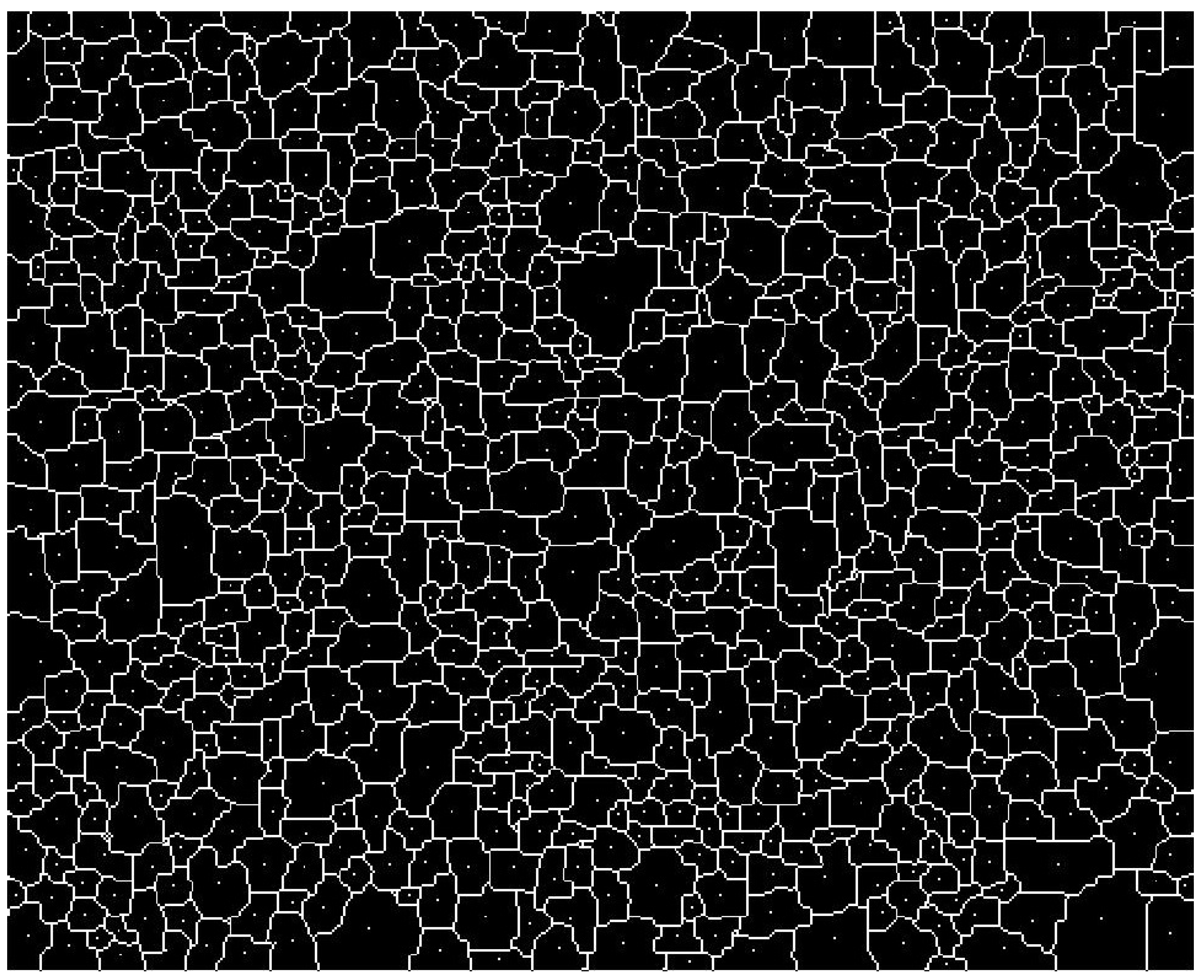
Multiresolution Segmentation

Using the business image processing software eCognition, the FNEA (Fractal Net Evolution Approach) multiresolution segmentation was conducted on Image I. The scale parameter is empirically set as 3.0, the shape parameter is set as 0.1, and the compactness as 0.5. Finally, we got 663 segmented objects as shown in Figure 2. Note that the Fe₂O₃-band in Image I was not involved in the segmentation process. This is because: as the only major element (or say rock-forming element), the incorporation of Fe₂O₃ may misguide FNEA to pay more attention to regional diagenesis, rather than metallogenesis.

(3)

Find the Centroid of Each Object

First, draw the minimum enclosing rectangle (MER) for each image object, and the centroids of the MERs will act as the centroids of the corresponding objects, see Figure 2. However, if the centroid falls on or outside the boundary of an image object, it will be recalculated in the following way: (i) generating the skeleton lines for each object; (ii) removing the suspension lines along the main skeleton line; and (iii) finding the midpoint of the main skeleton line, and taking it as the centroid of the corresponding object. Thanks to the skimage.morphology, numpy, and other Python packages, these processing steps can be easily implemented on a computer.

Finally, we note that image segmentation is the process by which an original image is partitioned into some homogeneous regions/objects [6], so the spectral features of the centroids can be used to represent the spectral features of the corresponding image objects. Our proposed algorithm is developed based on this assumption.

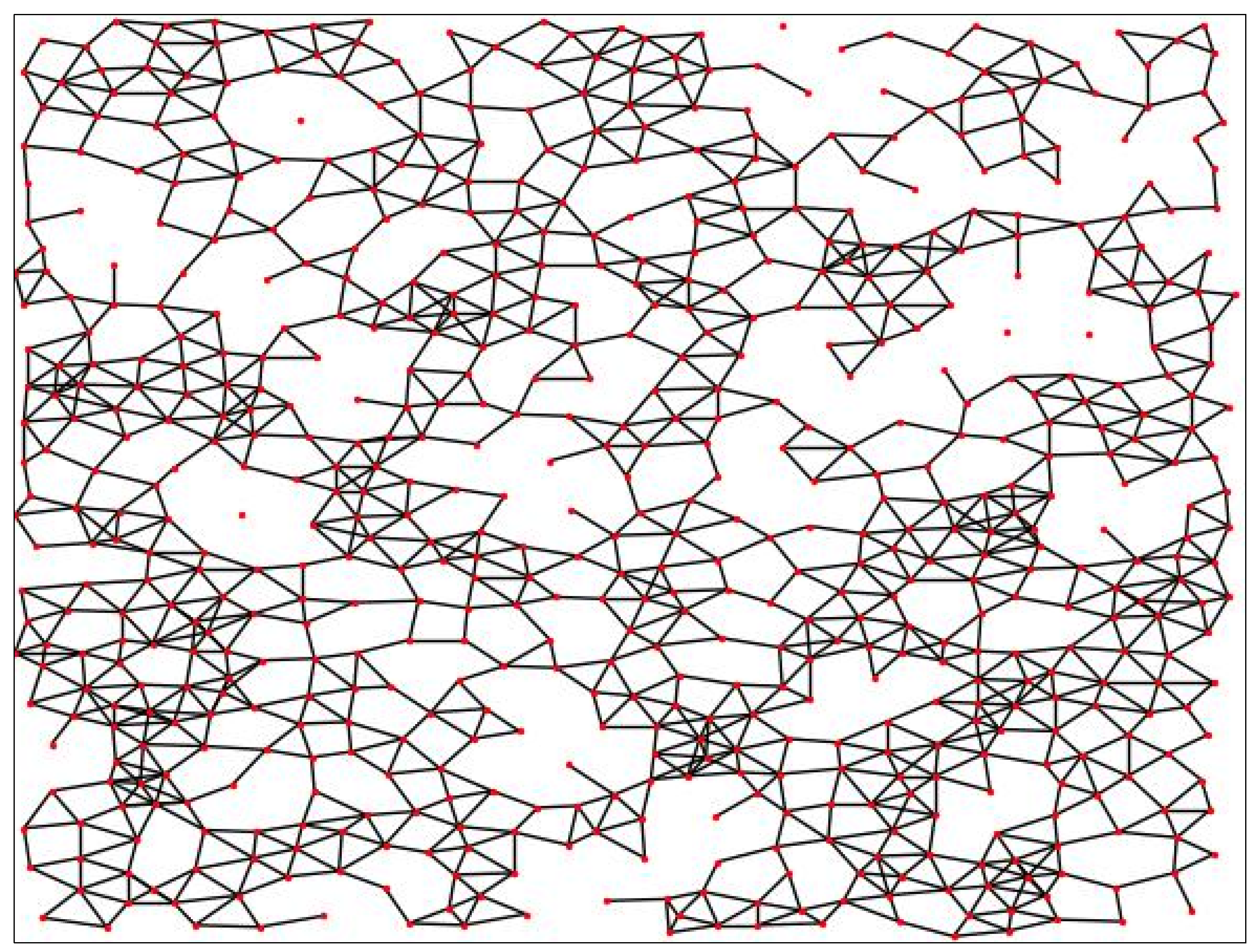
2.2.2. Constructing the Geochemical Topology Graph

As shown in Figure 2, the geochemical dataset can be collected as a group of centroids in an area. At the suggestion of [24], for regional geochemical exploration, only capturing the multivariable (multi-elemental) geochemical anomalies may be insufficient because their spatial distribution also reflects complex geological processes such as mineralization. To achieve this, the undirected graph (G) [24] which is used to connect closely related centroids to represent the spatial structure from point data is constructed as:

$$X=\{\overrightarrow{X_1}, \overrightarrow{X_2}, \dots , \overrightarrow{X_N}\},\overrightarrow{X_i}\in R^F$$

(1)

$$A=\left\{A_{1, 1}, A_{1,2}, \dots ,A_{N, N}\right\},A_{i, j}=\{\begin{array}{c}1, d_{i,j}\le K\\ 0, d_{i,j}>K\end{array}$$

(2)

where X and A represent the set of nodes/centroids, and edges, respectively; N represents the number of nodes in the graph; F denotes the number of features, namely geochemical variables (elements), of each node; d_i,j denotes the spatial distance between node j and i; K represents the distance threshold when constructing the geochemical topology graph, and generally, the smaller the distance between these two centroids is, the more related they are [24]; 1—connected edge and 0—disconnected.

In our case, N = 663; F = 11, which means there are 11 I-series or S-series ore-forming elements; and K is determined by the global Moran’s I analysis according to [24].

Global Moran’s I is a measure of the overall clustering of the spatial data. Figure 3 gives the global Moran’s I values versus different distance bands of all the geochemical variables. According to [32], if the Moran’s I value decreases rapidly as the distance band increases, there is a strong dependency relationship between the spatial structure and distance; on the contrary, if the Moran’s I value decreases slowly as the distance band increases, this indicates a stable spatial structure [32]. Obviously, the inflection point of the curve can act as the optimal threshold K to balance partial heterogeneity (i.e., anomaly) and the background features. An edge connects two adjacent centroids when the distance between them is less than K, and remains disconnected otherwise.

It can be seen from Figure 3 that there is a clear turning point at about 20 km for most of the ore-forming elements. For insurance purposes, here we use K = 22 as the distance threshold to construct the geochemical topology graph for subsequent network training and anomaly detection. Figure 4 is the generated topology graph, and each node of it corresponds to F = 11 features or geochemical variables [33]. Obviously, such a topology graph integrates both the spatial structural features and multi-elemental concentrations for a group of centroids in a given area.

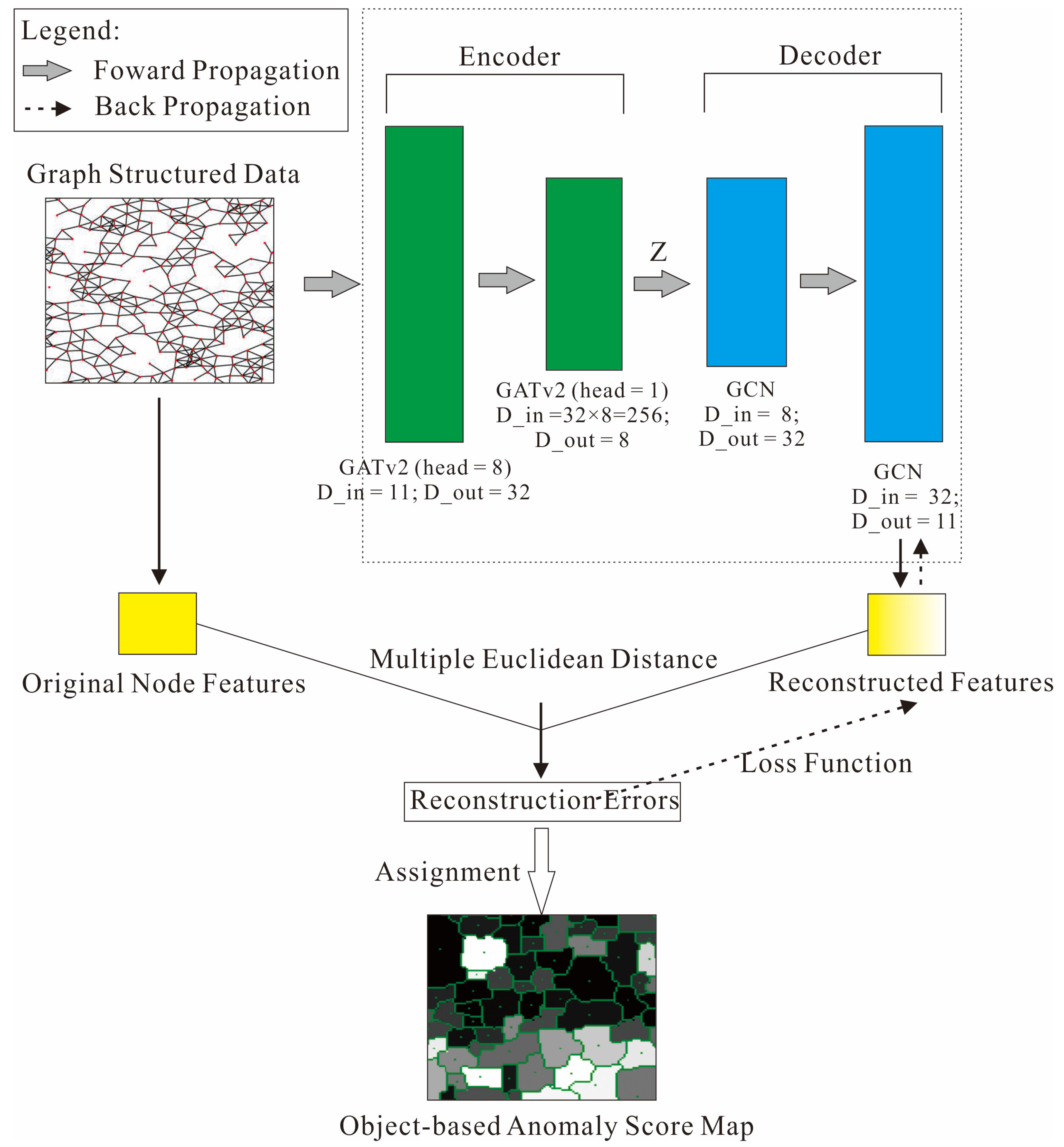
2.2.3. The Graph Network Architecture

Figure 5 gives the pipeline of the OGE architecture. Its basic components include a GAT-dominated encoder, a GCN-dominated decoder, the loss function, and so on. A detailed description of them is provided below.

(1)

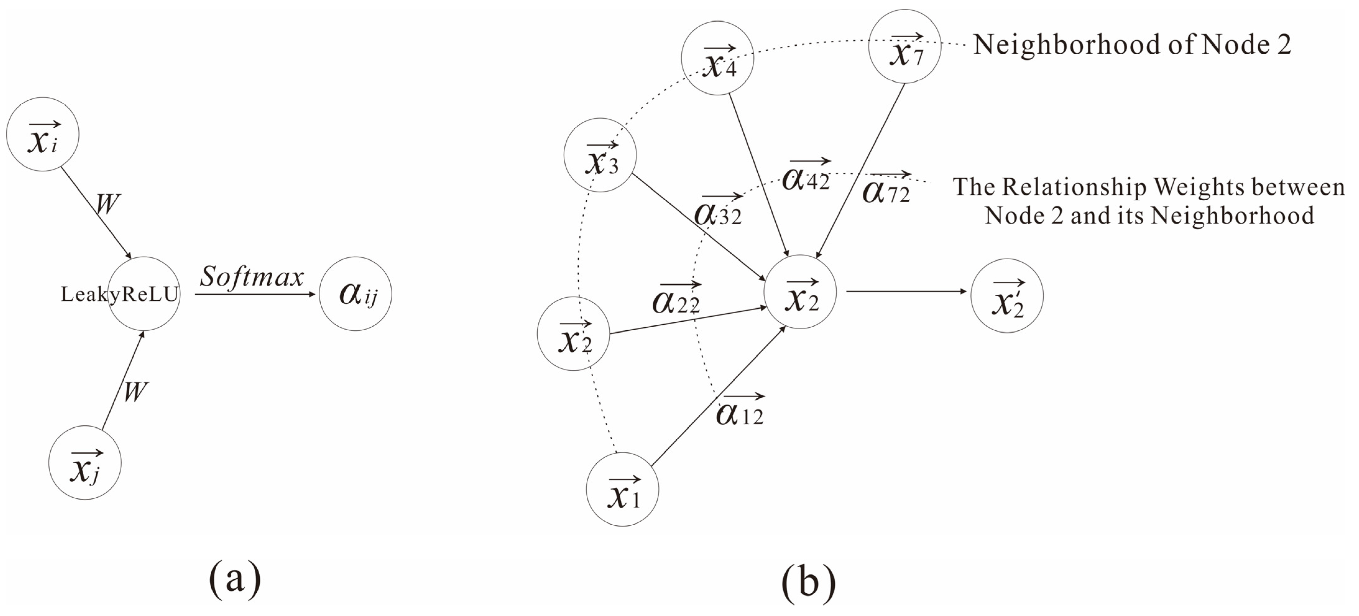
The GAT-Dominated Encoder.

GAT is one of the most popular GNN (Graph Neural Network) architectures and is considered as the state-of-the-art architecture for representation learning with graphs [33]. As illustrated in Figure 6, GAT is a two-step procedure: first, it calculates the attention coefficients (or say weights) of each graph edge according to the masked attention mechanism; afterwards, it aggregates the neighboring node features according to their weights [27].

Given an input topology graph G (X, A) containing N nodes/centroids, each node has a feature vector $\overrightarrow{x_i}$ and dimension F. The attention coefficients α_ij between nodes i and j is calculated as:

$$\begin{array}{ll}{\alpha }_{ij}& =softmax(attention(W·\overrightarrow{x_i}, W· \overrightarrow{x_j}))\\ & =softmax(LeakyReLU({\overrightarrow{a}}^T[W·\overrightarrow{x_i}|| W·\overrightarrow{x_j}]))\end{array}$$

(3)

where attention() represents a single-layer feedforward neural network with a weight vector $\overrightarrow{a}$; W represents the weight matrix for transforming the input features into higher-level features; ^T and || represent the transposition and concatenation operations, respectively; LeakyReLU is a non-linear activation function; and softmax() is used to normalize the neighbors of node i between 0 and 1.

After that, GAT aggregates each neighboring node and obtains the embedded features as follows:

$$\overrightarrow{{x_i}^{\prime }}=\sigma \left({\displaystyle \sum }_{j\in N_i}{\alpha }_{ij}·W·\overrightarrow{x_j}\right)\overrightarrow{x_i}\in N_i$$

(4)

where $\overrightarrow{x_i}$ and $\overrightarrow{{x_i}^{\prime }}$ represent the input data and embedded features, respectively; σ-sigmoid() is used to normalize the output between 0 and 1; N_i denotes the neighbors of node i. From the geological point of view, the geochemical signatures of mineralization-favored spaces inherited from multiple geochemical processes are often anisotropic [7], and Formula (4) indicates that the anisotropy of the node i in terms of geochemical signatures can be characterized by the relationship weights α_ij of node i’s neighborhood points {x_j, j = 1, 2, …, N_i}, including itself, see Figure 6b.

Authors in [34] further pointed out that: in GAT, every node attends to its neighbors given its own representation as the query, but for any query, the neighbor-scoring is monotonic with respect to per-node scores. This could be problematic in real-world applications. To remove this limitation, they proposed GATv2 by just modifying the order of operations in GAT. Their experiments demonstrated that GATv2 outperforms GAT in all benchmarks while having the same parametric cost. Inasmuch, as shown in Figure 5, this study used two GATv2 layers to construct the encoder of OGE, and then, the input geochemical topology graph is learned and mapped to a low-dimensional vector space Z. Our encoder can seamlessly learn the compositional relationships of eleven geochemical variables (i.e., nodal attributes) and their spatial structural features. On the contrary, traditional encoders (backbone networks) based on convolutional layers or self-attention can only process data with regular spatial arrangements, and they cannot be applied to extract features from graph structured data.

(2)

The GCN-Dominated Decoder.

GCN is a type of convolutional neural network that can work directly on graphs and take advantage of their structural information [33]. To put it simply, for each node, first we get the feature information from all its neighbors including itself, and then, we take the average of all its neighbors (assuming we use the average() function), after that, these average values will be feed into a fully connected neural network [33]. Note that in practice, we usually use more sophisticated aggregate functions rather than average(). In Figure 5, a GCN-based decoder, which is symmetric to the encoder architecture, was proposed to reconstruct the nodal attributes from the encoded latent representations Z. Finally, we use the sigmoid() function to restrict the reconstructed background values within the range of [0, 1].

Maybe it is better to use GAT layers to construct the decoder structurally symmetric to the encoder. If so, D_out of the second GAT layer in the decoder must be divisible by the number of nodal features (11), or say D_out * 8 (the number of heads) must be equal to 11 and D_out must be an integer, but it is obviously not possible in our case. So instead, GCN was applied to obtain the nodal reconstructed features.

(3)

The Loss Function.

Our OGE is an unsupervised machine learning approach, so its loss function does not involve manually annotated labels. At the suggestion of Guan et al. [24], here we use the unsupervised SPRE (i.e., sampling point reconstruction error) function as our loss function, which is formulized as:

$$L_{SPRE}=\frac{1}{N}{\displaystyle \sum }_{i=1}^N{A}_i$$

(5)

$$A_i=\sqrt{{\displaystyle \sum }_{k=1}^F{\left(x_i^k-{x^{\prime }}_i^k\right)}^2}$$

(6)

where $x_i^k$ and ${x^{\prime }}_i^k$ represent the kth original and reconstructed nodal features of ith node, respectively; N and F denote the number of nodes/centroids and variable categories, respectively; A_i denotes the reconstruction error (or say the anomaly score) for each centroid, namely the multivariate Euclidean distance between the original geochemical values and the reconstructed background values.

By minimizing the Formula (5), OGE can continuously learn the spatial structural features and compositional relationship from the input graph structured data by back propagation, and then approximate iteratively the input attributed graph with encoded latent features until the L_SPRE function converges [24]. After that, we input the original geochemical topology data into the trained model to obtain the reconstructed geochemical background values for each node or centroid. And then, we calculate the reconstruction error (namely A_i) for each node. Finally, the geochemical anomaly score map is generated by assigning the nodal reconstruction errors back to the corresponding image objects as the summary statistics. This process is summarized and pictured in Figure 5.

2.2.4. Data Post-Processing

After obtaining the object-oriented anomaly score map, we need a binarization threshold defining whether a given image object is anomalous or not. In this article, the threshold value is empirically set as the 50% quantile (median) of the object-oriented anomaly score matrix, which is 0.089434 for the I-type elemental association, 0.091733 for the S-type association, and 0.12807 for all the ore-forming elements.

In addition, as the anomaly score is an object-level summary statistics, so our post-processing operations will focus on the within-object statistical analysis as mentioned in the Introduction. From the geological perspective, differentiation-dominant processes are believed to be the pivotal cause of metallogenesis [30], and the fractal dimension (D) [15] is introduced here to describe the differentiation degree of each anomalous patch. As a within-object statistical parameter, D is used to quantify the power-law relationship between multi-elemental contents and their cumulative summation in a given image object. It can be computed and interpreted in the following way:

N(≥r) = Cr^−D (r > 0)

(7)

where r is the multi-elemental content value within an image object, and N(≥r) denotes the summation of content values larger than or equal to a given r; C > 0 is a proportionality coefficient, and the exponent D is known as the fractal dimension.

Mathematically, a number of straight-line segments (namely scaleless intervals) can be derived from Formula (7) on the log-log paper. It aims to cluster a dataset into most similar groups in the same segment and most dissimilar groups in different segments [15]. For two adjacent straight lines with different slopes, D_n & D_n+1, the inflection point (T) is routinely determined by RSS:

$$\mathrm{RSS}={\sum }_{\mathrm{i}=1}^{{\mathrm{i}}_0}{\left[\ln \mathrm{N}\left(r_{\mathrm{i}}\right)+{\mathrm{D}}_1\ln r_{\mathrm{i}}-\ln C_1\right]}^2+{\sum }_{\mathrm{i}={\mathrm{i}}_0+1}^{\mathrm{N}}{\left[\ln \mathrm{N}\left(r_{\mathrm{i}}\right)+{\mathrm{D}}_2\ln r_{\mathrm{i}}-\ln C_2\right]}^2\to \mathrm{Min}$$

(8)

where RSS denotes the “residual sum of squares”, and $r_{i_0}$ is the dividing threshold (namely T_n, n = 1, 2,…). In a similar fashion, the slopes of several scaleless segments, as well as the thresholds between them, can be quantitatively determined.

As shown in Figure 7, in this step, they are customarily classified into two segments, D₁ and D₂. According to Zhao et al. [15], the dimension D can be used to measure the clustering degree of a dataset, which is a diagnostic spatial distribution pattern for ore-related geological objects. The larger the D value, the steeper is the line, the greater is the rate of change in elemental content, the lower is the degree of clustering, and vice versa. Note that D₁ usually represents the low-content background information, and it does not change much over different image objects, so we use D₂ as an indicator to quantify the multi-elemental clustering. Suppose there are L pixels in an image object, and each object has F data layers representing different geochemical variables, and then, all of the L × F content values will be fed into the fractal algorithm aforementioned. As the selected elements are paragenetically associated with each other, and their content values are normalized to [0, 1] by subtracting the mean values, so if the metallogenesis or differentiation occurs, the content values of these elements within a given object will become more clustered, which corresponds to a smaller D₂; otherwise, they remain scattered because of the weak feature of elemental association, which corresponds to a larger D₂ value. In addition, we do not have to make a strict assumption that the multi-elemental contents follow a multi-fractal distribution when conducting the within-object statistical analysis, for the algorithm can adaptively process or yield new insights for those non-fractal data [35]. Finally, every image object will be assigned a dimension value that can be used to modify the anomalous regions delineated by OGE.

3. Results

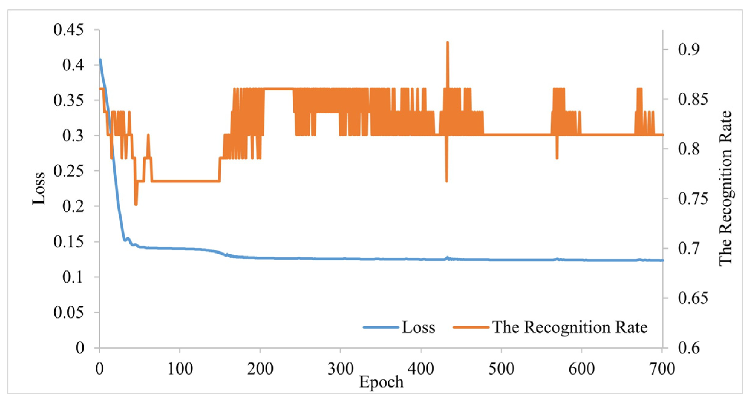
3.1. Implementation Details

We implement the proposed OGE model as well as the relevant pre- and post- processing using the Python framework which is open source. The most important packages involved in the programming experiments include but not limited to Pytorch, Pytorch Geometric, Numpy, Networkx, and so on. OGE was conducted on a single NVIDIA Tesla V100 with 32 GB of GPU memory and train for 2000 epochs to make the model converge. We use the Adam optimizer to train our models from scratch, and the initial learning rate is set to 0.005, and the weight decay coefficient is set to 0.0005 By the way, the primary purpose of regional geochemical exploration is to delimit areas of interest for further exploration, and thus, the performance of OGE can be evaluated or described from two perspectives: the percentage of discovered mineral deposits to the total mineral deposits—the recognition rate, and the size of the anomalous area.

For a better illustration, taking the I-series elemental association as example, Figure 8 gives the recognition rate versus loss curves during the training phase. As can be seen, before completing 160 epochs, both the recognition rate and the training loss decrease sharply. And then, the decreasing trend of loss become slow, eventually stabilizing at 0.124 or so; meanwhile, the growth of the recognition rate rises and became oscillating, centered at 0.837. So, in order to jump over the oscillation area, here we set the training epoch as 2000.

3.2. The Object-Based Anomaly Score Map

For the I-series elements, it can be seen from Figure 9 that: (1) most of the known ore spots/deposits, no matter what their scales and mineral species, fall within the image objects having higher anomaly scores (brighter colored areas). (2) Using the median value as the threshold, there are 30 ore spots falling within the delineated anomalous regions, and 13 spots falling outside. The recognition rate is 69.767%. (3) Using the 60th percentile value as the threshold, there are 26 ore spots falling within the Level I anomalies, and the recognition rate is 60.465%. (3) The Level II anomalous area accounts for 49.778% of the total area, and the Level I area accounts for 40.079%. (4) Many of the anomalous objects are barren, especially those on the northwest corner of the study area. (5) Most of the mineral spots except Au falling outside the anomalous regions occur nearby the anomalous boundaries. If we create a 4-pixel buffer zone around the Level II anomalous objects, there are only 4 ore spots falling outside, and the ore-spot recognition rate comes up to 90.70%. (6) If we create a buffer zone around the Level I anomalies, the recognition rate increases to 74.419%.

For the S-series elements, it can be seen from Figure 10 that: (1) there are 40 ore spots falling within the Level II anomalous regions, and only 7 spots falling outside. The recognition rate is 85.106%. (2) there are 33 ore spots falling within the Level I anomalies, and the recognition rate is 70.213% (3) most of the ore spots falling outside the anomalous regions occur nearby the anomalous boundaries, and relevant anomaly scores fluctuate between 0.030 and 0.070. If we create a 4-pixel buffer zone around the Level II anomalous patches, there are only one fluorite ore-spot falling outside, and the recognition rate comes up to 97.87%. (4) If we create a buffer zone around the Level I anomalies, the recognition rate increases to 78.723%. (5) The Level II anomalous area without the buffer zone accounts for 50.054% of the total area, and the buffered anomalous area accounts for 68.24%. (6) The spatial distribution of the anomalous regions in Figure 10 is generally consistent with that in Figure 9.

Figure 11 gives the anomaly score map of all the ore-forming elements, and we can observe that: (1) The Level II anomalous area accounts for 49.881% of the total area. (2) There are 50 ore spots falling within the Level II anomalous regions, and 18 ore spots falling outside. (3) The recognition rate of the Level I anomalies is 66.176%. (4) In the buffered anomalous area, only 8 mineral spots falling outside, and the recognition rate increases to 88.24%. (3) Only a few ore spots fall within the image objects with the brightest tone, namely with the largest anomaly scores.

Given the above, OGE’s performance on S-series elements is even better than that on I-Series elements. The main drawback of our methodology is that the delineated anomalous area is too large and many of the anomalous patches are barren, which is not helpful for guiding the follow-up anomaly verification. As stated before, these results may demonstrate the possible pitfalls of using object-level anomaly scores due to their possible misrepresentation of the within-object geochemical characteristics [10]. That is to say, the anomalies delineated by OGE must be further modified through the within-object multi-elemental statistical analysis.

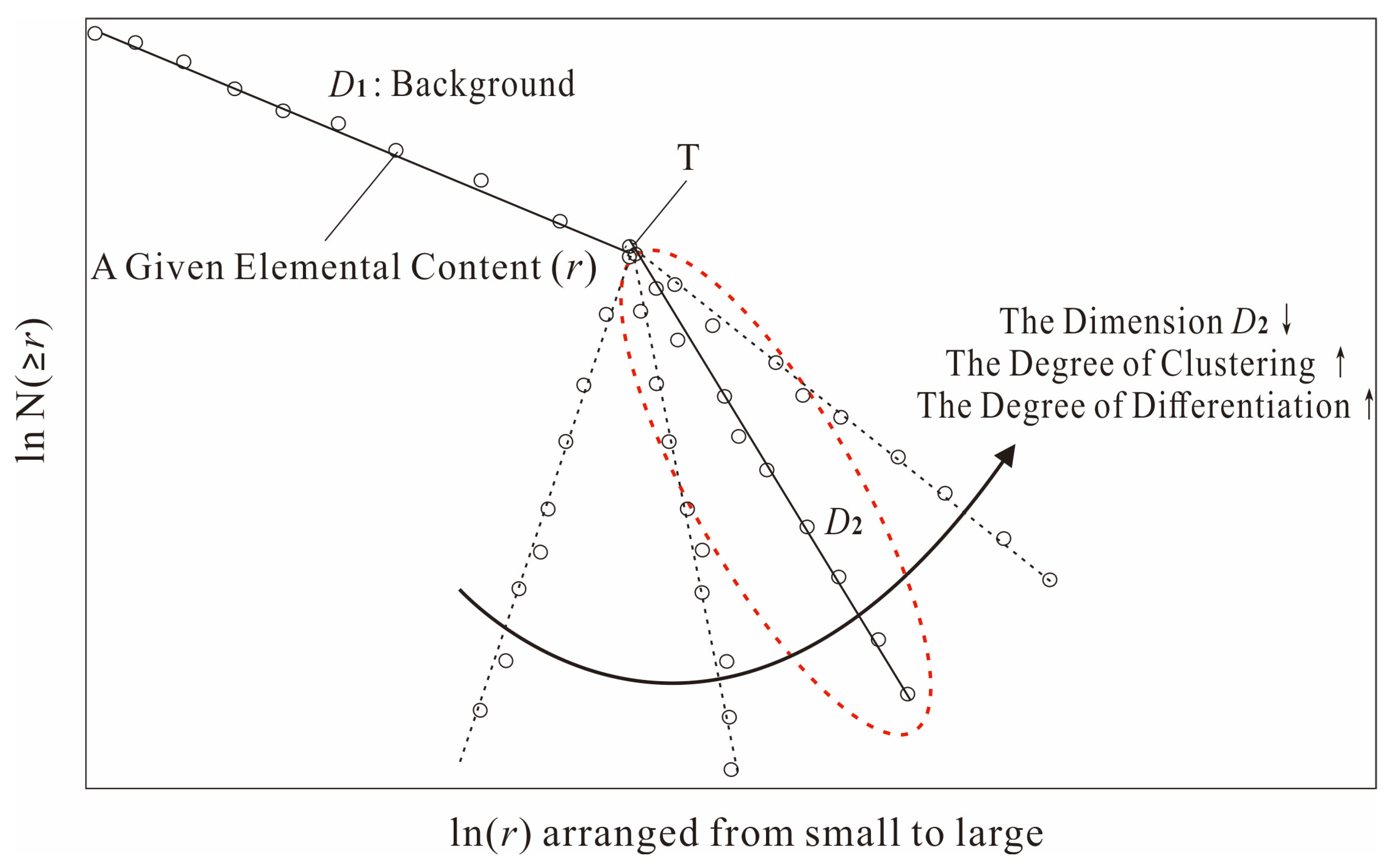
3.3. Elemental Within-Object Separability

Figure 12 gives the object-based map of dimension (D₂) for the I-series and S-series elemental associations, respectively. We note that as the geochemical behaviors of the I-series elements are quite different from those of the S-series elements [30], so the object-based D₂ map for all elements was not calculated here. From Figure 12 and Figure 13, we have delivered three important observations as follows:

(1)

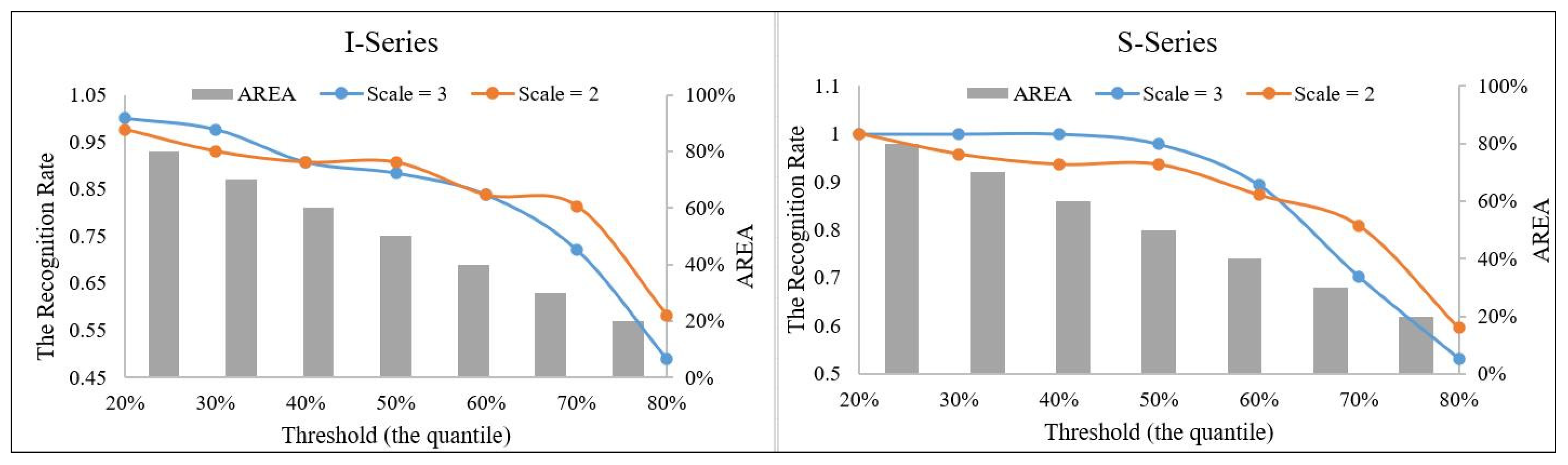
The D₂ values of the image objects containing the known ore spots vary in a wide range. For the I-series ore spots, the relevant dimension values fluctuate between 2 and 116 with a peak at 18 (The original D₂ values were normalized to [0, 255]), and if we set D₂ = 116 as the binarization threshold, the obtained anomalous area accounts for 98.63% of the total area. For the S-series ore spots, the relevant dimension values fluctuate between 1 and 32 with a peak at 14, and if we set D₂ = 32 as the threshold, the obtained anomalous area will account for 78.93%.

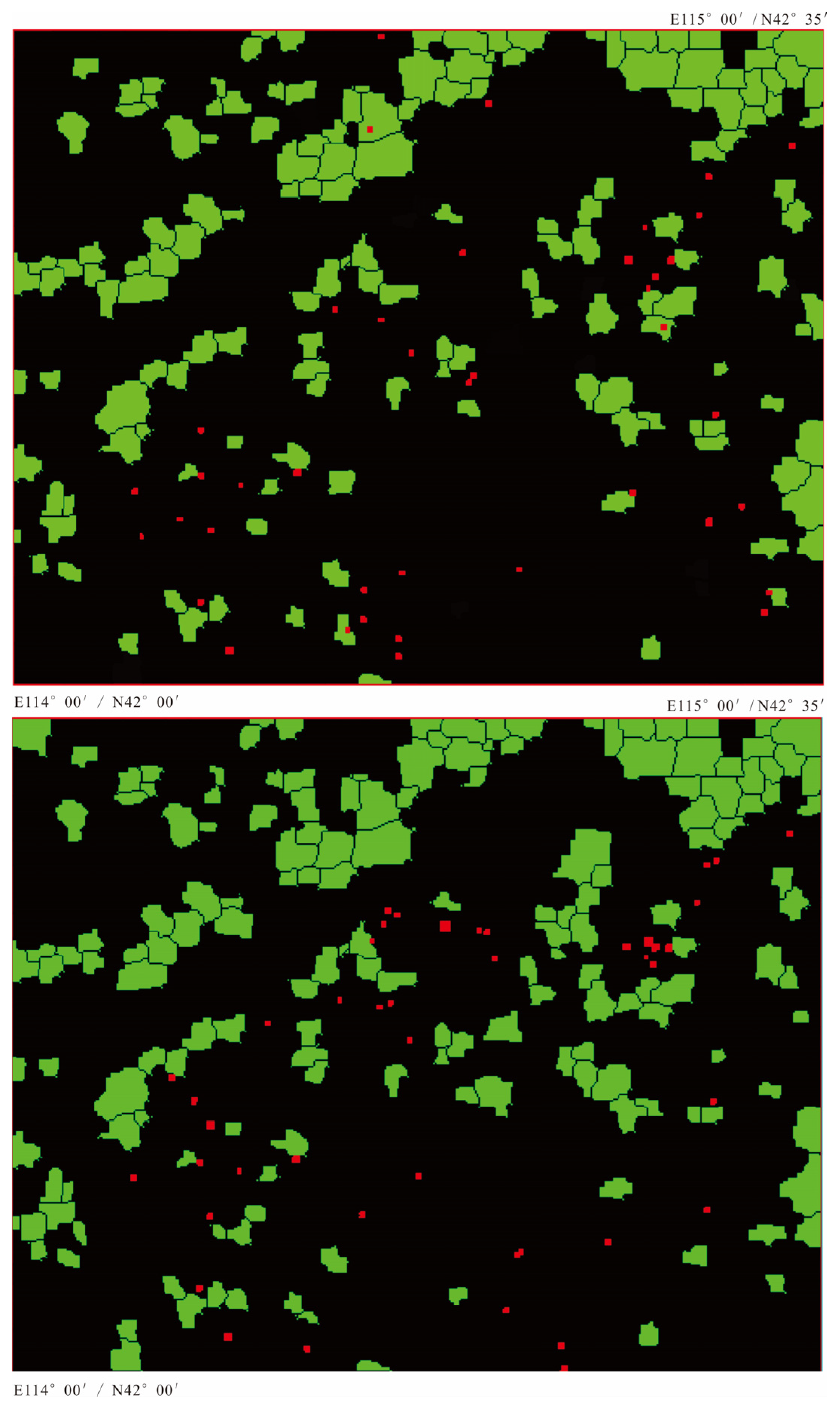
(2)

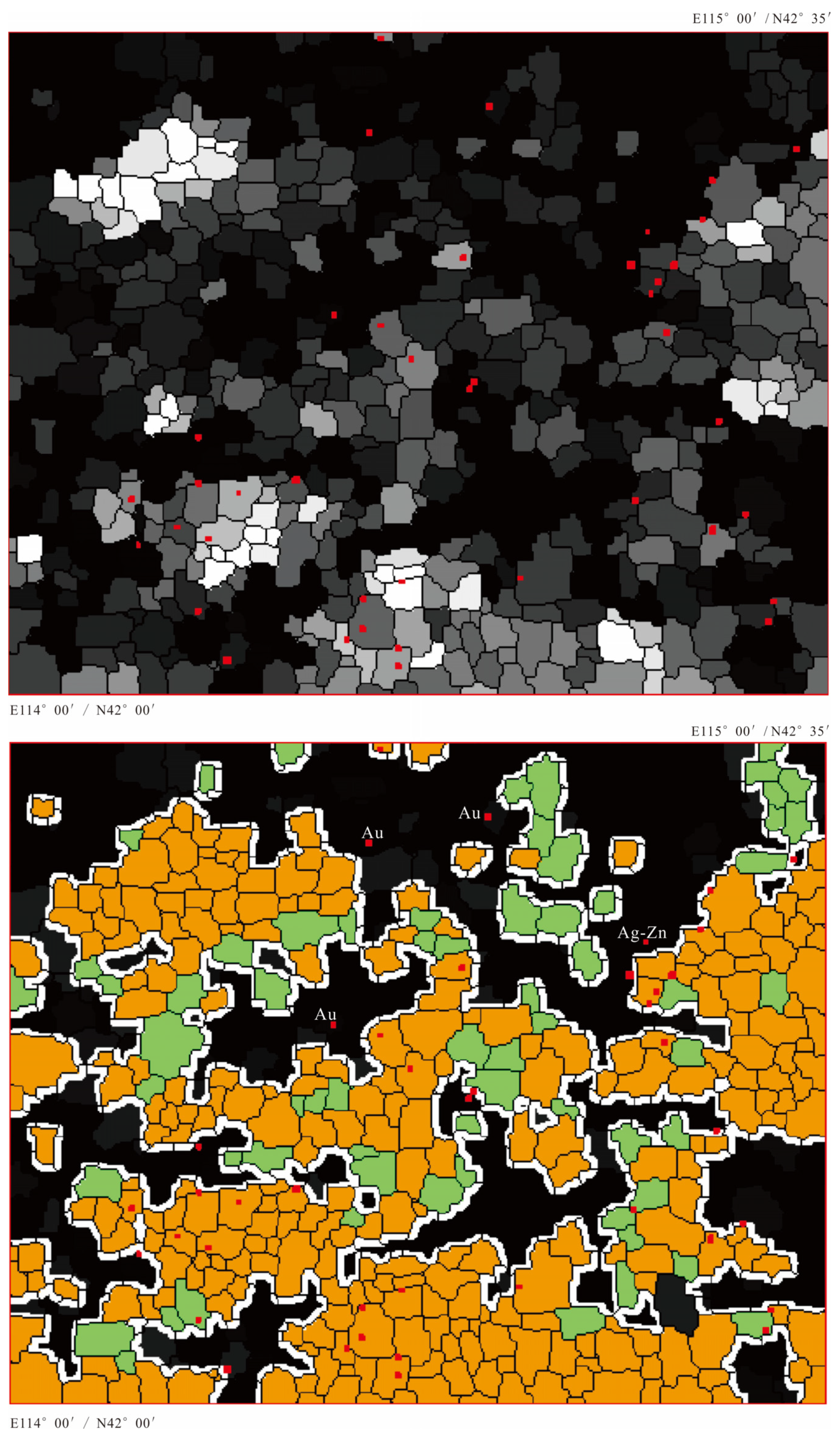
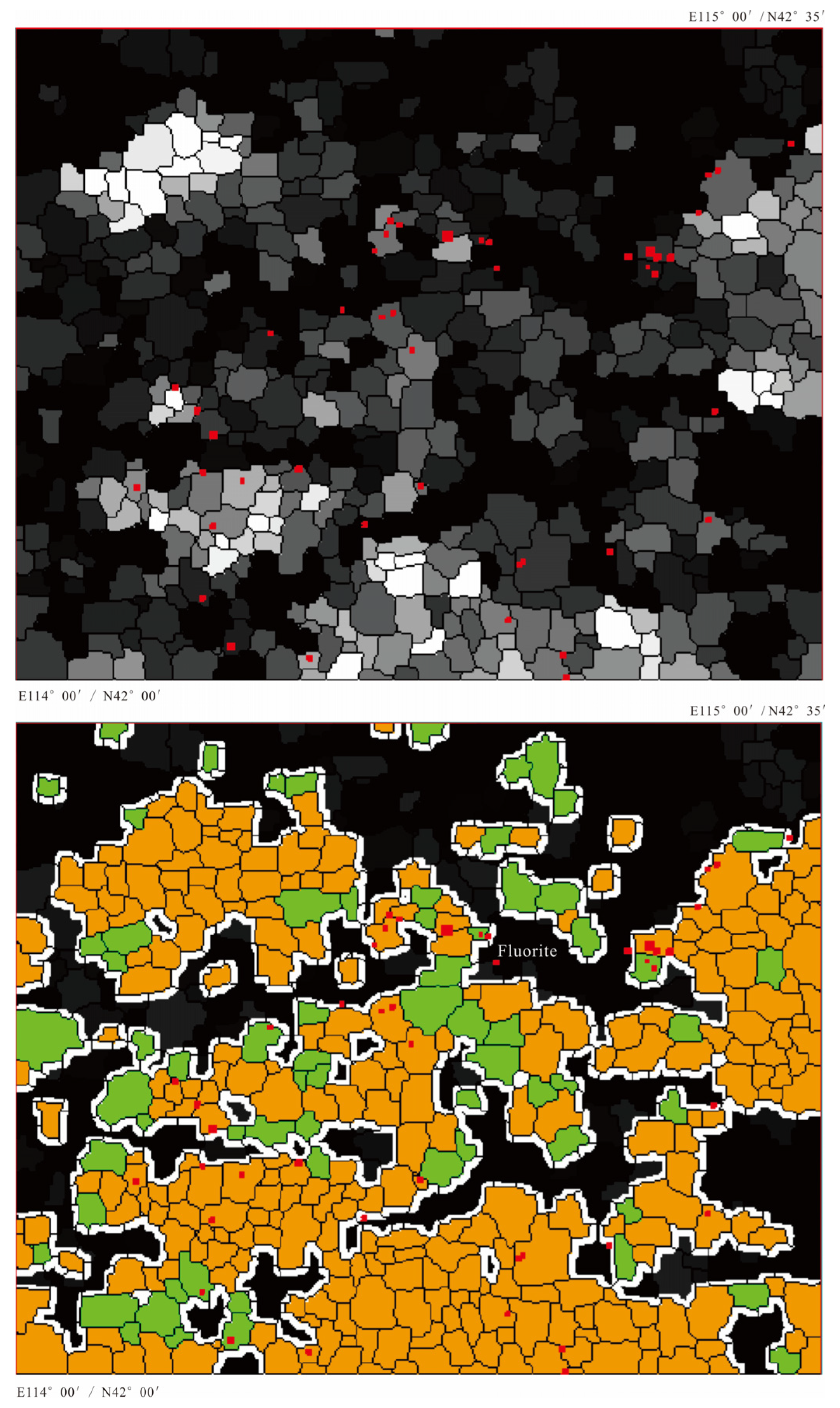
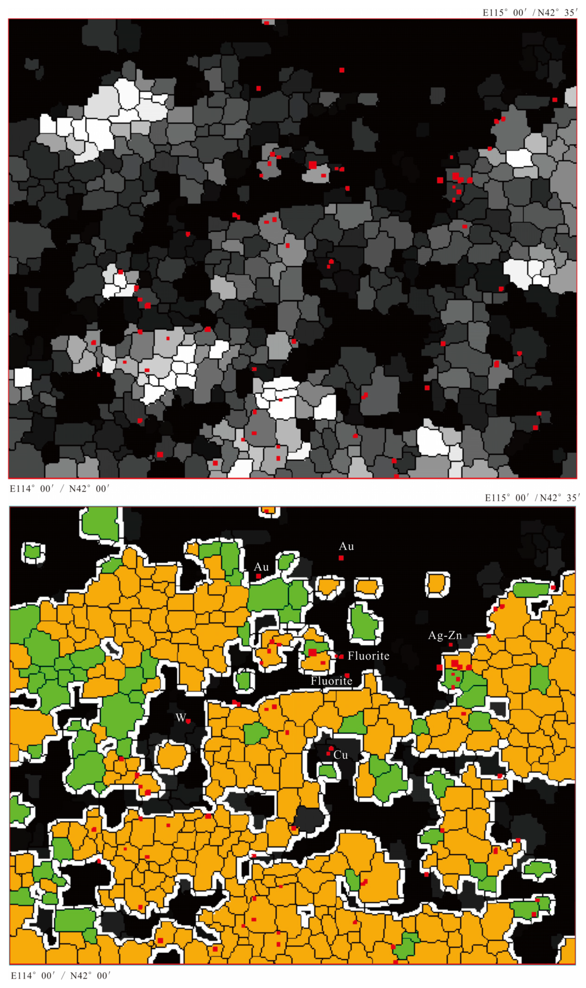
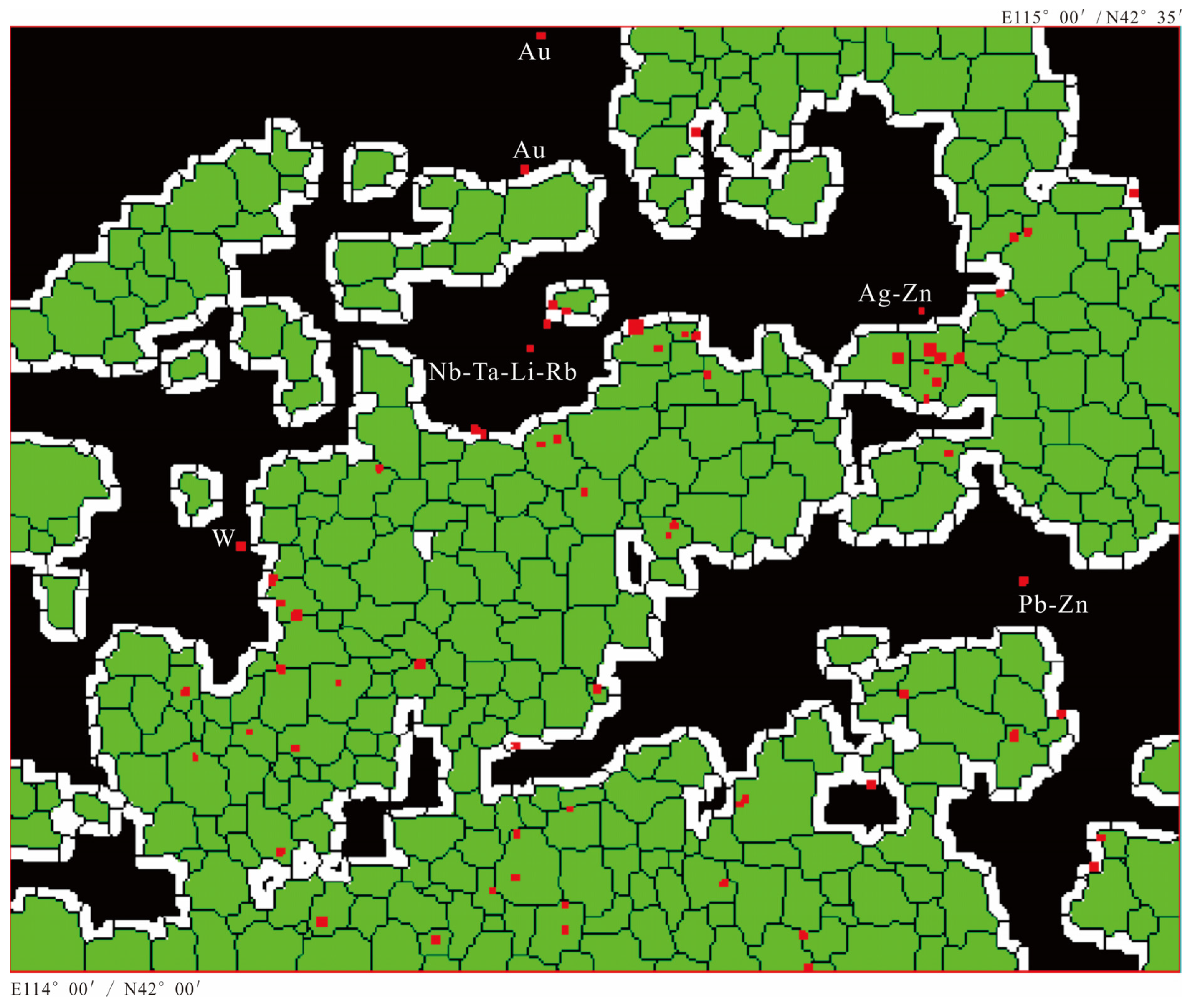
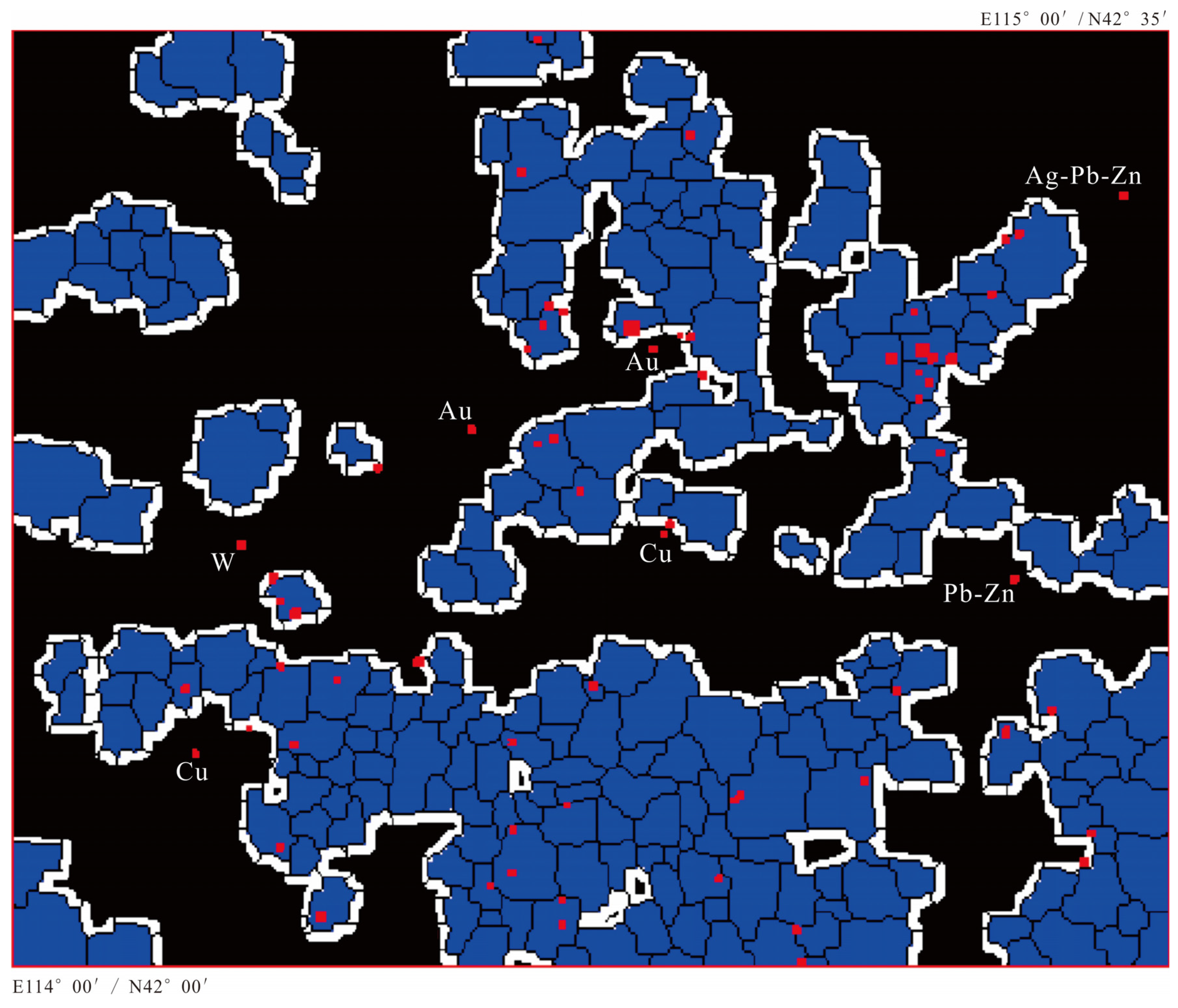
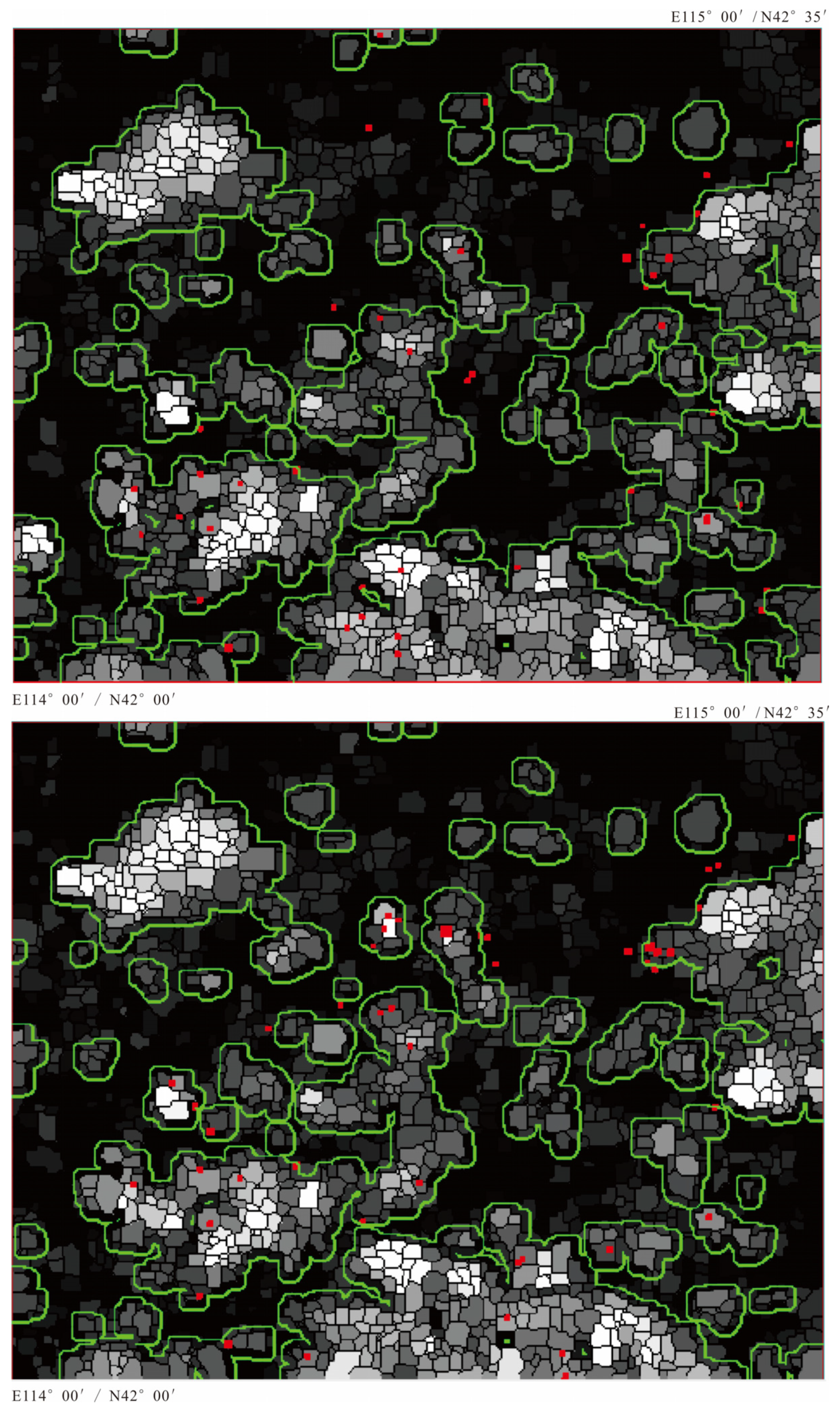
As the histogram of the D₂ map is usually right-skewed, so we empirically set the binarization threshold as the mode value + 1 × standard deviation (for a standard normal distribution, 68.3% of data falls within one standard deviation of the mean, so we suppose that most, if not all, of the ore-spots would fall within the objects with the D₂ value ≤ mode + 1 × standard deviation). For I-series elements, the threshold is 36, and for S-series, it is 34. Our purpose of image binarization is not to delineate the anomalous regions like Figure 9, Figure 10 and Figure 11 do, but to delineate some highly confident non-anomalous objects. That is why in Figure 12, very few ore-spots fall in the colored patches. Naturally, by removing these non-anomalous objects from Figure 9 and Figure 10, we can obtain a moderately reduced prospecting-target-area as shown in Figure 13.

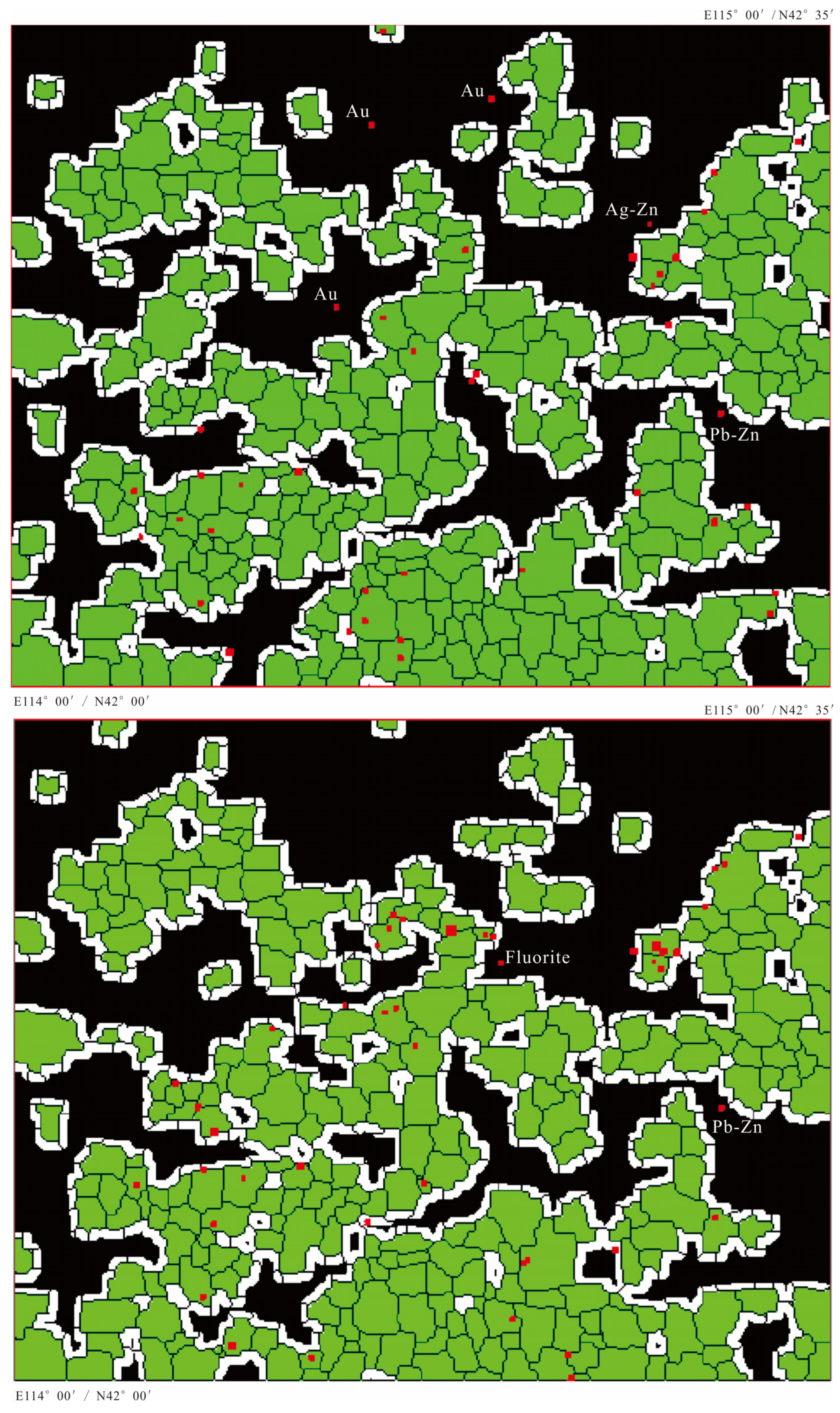
(3)

In Figure 13 (upper), the anomalous area of I-series elements decreases to 43.045% of the total area, and the buffered anomalous area decreases to 61.608%. Only 5 ore-spots fall outside the reduced anomalous target area, which are Au, Pb-Zn, and Ag-Zn mineral spots. In Figure 13 (lower), the anomalous area of S-series elements decreases to 43.172% of the total area, and the buffered area decreases to 61.534%. Only 2 ore-spots fall outside the target area, which are fluorite and Pb-Zn spots.

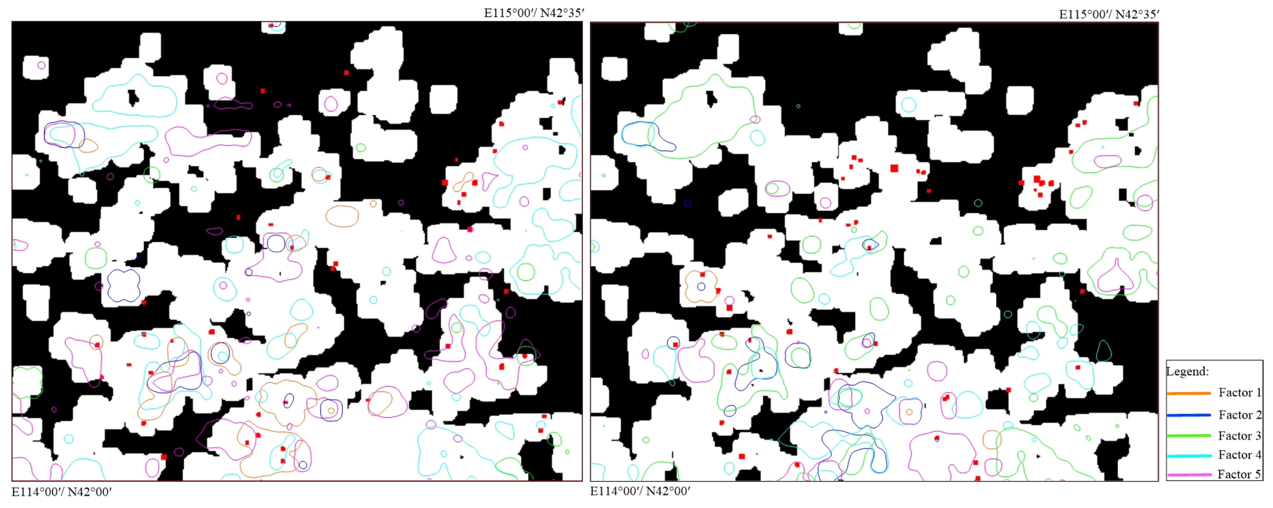
3.4. Comparison and Validation by Factor Analysis

The best way to validate the effectiveness of our OGE algorithm is to observe how many ore spots can fall into the anomalous image objects, but this is not enough because most of the anomalous patches in Figure 13 are barren. Comparing Figure 13 to Figure 1, we also discover that the presence of ore spots and anomalies is not completely controlled by the spatial distribution of the outcropped bedrocks and known geological structure. For example, over a third of the known ore spots occur within the N₂b and Quaternary-covered areas with less geological exposure. Inasmuch, it is difficult to directly validate the anomalies from the perspective of regional geology. In this Section, the factor analysis is used to do so. As we know, factor analysis is a well-validated technique that is widely used to reduce a large number of variables into fewer numbers of factors [32]. Although irrespective of the spatial structure of geochemical patterns, it facilitates the identification of multivariate geochemical anomalies. This is consistent with the major aim of OGE. So, supposing the results of factor analysis are tenable and close to truth, we can cross-validate the correctness and robustness of our model’s outputs by observing if the factor-score anomalies overlap considerably with the anomalies delineated in Figure 13.

We can make the following observations from Figure 14: (1) Nearly all the factor-score anomalies, no matter what the elemental association each factor represents, reside within the OGE-derived anomalous areas, and occupy most of the interior space. This result strongly supports the basic correctness of our model’s outputs. (2) Our OGE model is advantageous since quite a few ore spots that cannot be identified by the factor-score anomalies are well-identified by OGE. (3) The I-series elemental association can be further divided into five factors: Factor 1: As-Pb-Zn, Factor 2: Ag-B-Cu, Factor 3: Au-Hg, Factor 4: Mo-U, and Factor 5: Fe₂O₃. Likewise, the S-series elements can be divided into: Factor 1: Bi-W, Factor 2: Pb-Sb-Sn, Factor 3: Mo-U, Factor 4: Nb-Fe₂O₃, and Factor 5: Be-F. These divisions improve the interpretability of the extracted anomalies and facilitate the mineral species-specific geochemical exploration.

Given the above, by calculating the ore-spot recognition rate and conducting factor analysis, the OGE-derived anomalies in Figure 13 get validated.

4. Discussion

In our opinion, there are six meaningful aspects around the proposed network architecture worth to discuss, which are listed in the following paragraphs.

First, many factors, e.g., steep topography, the weathering and transportation of chemical compositions in stream sediment samples, surface hydrological processes, etc., can cause displacement of geochemical anomalies from the source area [7], and that is why most of the mineral spots falling outside the delineated anomalous regions occur nearby them. Inasmuch, it is highly necessary to create buffer zones for the known anomalous regions, although the total anomalous area increases accordingly.

Second, Figure 15 gives the anomalous score map using the geochemical dataset consisting of seven major rock-forming elements (Fe₂O₃, Al₂O₃, SiO₂, MgO, Na₂O, K₂O, and CaO) as input to OGE. Here we suppose that the anomalies delineated in Figure 15 reflect the regional diagenesis. It can be seen from Figure 15 that only 6 ore-spots fall outside the anomalous regions, and the ore-spot recognition rate is as high as 91.176%, exceeding Figure 11’s 88.24%. The spatial distribution of the anomalous regions in Figure 15 is also consistent with that in Figure 9, Figure 10 and Figure 11. Obviously, owing to the strong control of bedrock geology may exert on the chemical composition of stream sediments or soil samples, the determination of geochemical anomalies can be heavily affected by the lithology background in areas with variable lithologies. That is to say, the mineralization is attached to the diagenesis, and the delineated anomalies in Figure 9, Figure 10 and Figure 11 primarily reflects the regional diagenesis, and, to a lesser extent, the mineralization. Zhao et al. [36] further pointed out that, due to the lower spatial resolution, the 1:200,000 geochemical data cannot directly link to small-/medium-scaled ore occurrences, especially the micro-mineralization outcrops. Worse still, taking the image objects as basic analysis units tends to accentuate these trends rather than mitigate them. These explained why our delineated anomalous area is so large and is largely controlled by the outcropped bedrocks as displayed in Figure 1.

Third, in the within-object analysis stage, we use fractal dimension D₂ to measure the degree of multi-elemental clustering, but its performance in terms of reducing the prospecting-target-area is not as good as expected. We also observed that: the overall distribution pattern of the multi-elemental contents of the “pixels” in an object is usually right-skewed, thus it can be approximately modelled by a bimodal Gaussian distribution: one population deals with the normally distributed part, and the other one deals with the long right tail—although sometimes it is multi-peaked. And then, we can separate them and obtain their shape parameters, namely m₁ and m₂: the mean values of two adjacent Gaussian distributions, respectively, and m₁ < m₂; σ₁ and σ₂: the corresponding standard deviations. On this basis, the separability (J) [37] is calculated as:

J = 2(1 − e^−B), J∈[0, 2],

(9)

$$B=\frac{1}{8}{\left(m_1-m_2\right)}^2\frac{2}{{\sigma }_1^2+{\sigma }_2^2}+\frac{1}{2}\ln \left[\frac{{\sigma }_1^2+{\sigma }_2^2}{2{\sigma }_1{\sigma }_2}\right]$$

(10)

If the metallogenesis or differentiation occurs, the multi-elemental content values within an image object will have a small separability because of the strong feature of elemental association; otherwise, they will have a larger J value.

Unfortunately, like the case in Figure 13, only a moderately reduced prospecting-target-area was generated based on the object-oriented J map. These experiments imply that: D₂, J, as well as other manually designed features may not be a good indicator to separate multi-elemental anomalies from background, and alternatively, deep features produced by, e.g., OGE usually perform well in this case.

Fourth, the delineated anomalous area can be dramatically reduced by increasing the binarization threshold. For example, for the S-series elements, when setting the binarization threshold as the 60% quantile (0.10562), the anomalous area decreases to 40.005% of the total area, but 6 ore-spots are excluded from the buffered anomalous regions; when setting the threshold as the 70% quantile (0.12625), the anomalous area decreases to 29.872%, but 14 ore-spots are excluded; when setting the threshold as the 80% quantile (0.16079), the anomalous area decreases to 20.157%, but 22 ore-spots are excluded; when setting the threshold as 0.2202 – the 90% quantile, the anomalous area decreases to 10.022%, but 34 ore-spots fall outside the buffered anomalous regions, and only 13 ore-spots fall within. The case is similar for the I-series elements. That is to say, the anomaly scores of the ore-containing image objects vary in a wide range, from the 50% quantile to 100%. In our opinion, this can be mainly attributed to the low resolution of the geochemical data in use and its weak ability in detecting the micro-mineralization outcrops. To prove this, Figure 16 further gives the anomalous regions extracted by 1:50,000 soil/stream-sediment survey data, which is generated using the geochemical dataset consisting of 12 ore-forming elements (Ag, As, Au, Bi, Cu, Hg, Mo, Pb, Sb, Sn, W, and Zn) as input to OGE. In Figure 16, we raise the binarization threshold from the 50% quantile (median) to the 60% quantile, and the anomalous area decreases to 38.11% of the total area accordingly. Comparing to Figure 11, a 11.77% reduction in anomalous area has been achieved without affecting the recognition rate: only 7 ore-spots fall outside the buffered anomalous area. If we raise the threshold to the 70% quantile, the anomalous area decreases to 29.54%, and only 11 ore-spots fall outside (the recognition rate remains above 80%). Obviously, due to the improved spatial resolution, our OGE model is guided to focus more on regional mineralization, rather than diagenesis.

Fifth, in the pre-processing stage, first we interpolate sampled point data into raster grids, and then, they are aggregated into different image objects, which inevitably introduces uncertainties into the data. Naturally, people may question if a reduced segmentation scale can help improve the anomaly-detection performance. To answer this question, we use the scale parameter 2.0 to segment the input geochemical image, and finally we get 2465 objects as displayed in Figure 17. Taking the S-series elements as example, comparing to Figure 10 (upper), more details about the anomalies have emerged, but their spatial distribution patterns are generally consistent with those in Figure 10. We still have to set the binarization threshold as median to keep the ore-spot recognition rate greater than 90%, whereas if we raise the threshold to the 70% quantile, only 9 mineral spots fall outside the buffered anomalous area, and the recognition rate remains greater than 80%. Figure 18 gives the big picture: when we set the threshold smaller than or equal to the 60% quantile, the OGE analysis performed at higher levels of scale has higher recognition rate; whereas when we set the threshold greater than the 60% quantile, lower levels of scale may perform better. Figure 17 is such an example: when the threshold is set as the 70% quantile and the scale parameter is set as 2, 81.4% of the I-series mineral spots can fall within the corresponding buffered-anomalous-area which accounts for <45% of the study area, and 80.9% of the S-series ore spots can be included. By contrast, if the scale parameter increases to 3, only 72% of the I-series ore spots and 70% of the S-series ore spots can be included in the relevant anomalous areas. Given the above, in order to balance the recognition rate and anomalous area, it is better to use a smaller scale parameter to segment the multivariable geochemical image.

Sixth, as our OGE architecture was developed as an updated version of GAUGE by combining OBIA and GNN (GAT & GCN) into a singular network, so it is necessary to compare the performance between them. As shown in Figure 19, which is generated by using the geochemical dataset consisting of all 18 ore-forming elements as input to GAUGE, we found that the spatial distribution patterns of the anomalous areas are generally accorded with those in Figure 11, but more details have emerged; if setting the binarization threshold as the 50% quantile, there are more than 19 ore-spots falling outside but being close to the anomalous regions; if setting the threshold as the 70% quantile, there are 25 missed ore-spots. As far as the recognition rate is concerned, the performance of GAUGE is no better than OGE. Nevertheless, even the threshold is set as the 70% quantile, most of the missed ore spots could fall within the 2 km (i.e., the controlling distance of one sampling point) buffered anomalous regions, and the ore- spot recognition rate approaches 100%. However, the resulting anomalous area will increase to >75% of the total area. In addition, the within-object statistical analysis is not supported by GAUGE. Given the above, our OGE performed better in anomaly detection: in Figure 17, more than 80% of the known ore spots were predicted in the buffered anomalous area accounting for less than 45% of the total area. In fact, both GAUGE and OGE were designed to extract both the spatial features and compositional relationships of geochemical variables collected at irregularly distributed locations. For OGE, such irregularity is implemented by the multiresolution segmentation whose output is a series of irregularly distributed centroids in irregularly shaped image objects [6], which may reflect the variation of geochemical background across the space. On the other hand, as shown in Figure 19, the sampling grid is relatively regular, and very few geochemical sampling points are missing in this area. This implies that GAUGE could not capture the practical spatial distribution characteristics of geochemical variables, which reflects complex geologic processes (i.e., mineralization). That is why the visual performance of GAUGE is not as good as expected. Other convolutional autoencoder models available in the literature, such as SCMA (Spatially Constrained Multi-Autoencoder) [38], were not discussed here because they cannot be applied to an irregular area for anomaly identification.

From the above, it is still difficult for us to reduce the anomalous area to below 30% of the study area. However, previous studies on separation of geochemical anomalies in the literature mainly focus on a singular mineral species, while our study seeks to delineate the all-mineral-species anomalies. In this sense, a relatively large anomalous-target-area may be necessary.

5. Conclusions

The main contribution of this article is fourfold as follows: (1) to the best of our knowledge, this is the first time that the OBIA framework has been applied in regional geochemical prospecting; (2) a novel GNN architecture (OGE) has been designed to extract multi-elemental geochemical anomalies which can locate most of the known ore spots, no matter what their scales and mineral species; (3) for the first time the within-object multi-elemental statistical analysis has been conducted to modify the anomalous regions delineated by object-level summary statistics; and (4) most studies on separation of geochemical anomalies in the literature focus on a singular mineral species, while our study attempts to delineate the all-mineral-species anomalies.

Taking the 1:200,000 stream-sediment geochemical survey data in the Bayantala-Mingantu district, North China as case study, our findings indicated that:

(1) Most of the ore spots falling outside the delineated anomalous regions occur nearby them. (2) Due to the low resolution of the geochemical data at hand and its weak ability in detecting the micro-mineralization outcrops, the anomalous area produced by OGE is relatively large and mainly reflects the regional diagenesis. (3) The within-object statistical analysis based on handcrafted features, e.g., D2 and J, has a limited effect on reducing the anomalous target area. (4) OGE can be guided to focus more on regional mineralization, rather than diagenesis, by using fine-scale geochemical data as input. (5) Smaller segmentation scales can greatly improve the application of OGE. Finally, more than 80% of the known ore spots were predicted in less than 45% of the study area. (6) OGE is designed to extract both the spatial features and compositional relationships of geochemical variables collected at irregularly distributed centroids in irregularly shaped image objects, and it performs slightly better in anomaly detection than other convolutional autoencoder models such as GAUGE.

Future research will focus on improving the OGE in the following respects: (1) to alleviate the spatial heterogeneity of geochemical backgrounds, it is better to conduct the mean removal operation within every image object, rather than removing the global mean values for each element. (2) The optimal segmenting scale can be determined by using the ESP (estimation of scale parameter) tool proposed in [39]. (3) The possible approaches of integrating multiple datasets (e.g., remote sensing data and geophysical data) in the framework of OGE will also be explored. (4) Improve the within-object statistical analysis method, so that those strong but false or meaningless anomalies can be eliminated, while retaining those weak but important or meaningful anomalies.

References

1. Grunsky, E.C.; Drew, L.J.; Sutphin, D.M. Process recognition in multi-element soil and stream-sediment geochemical data. Appl. Geochem. 2009, 24, 1602–1616. [Google Scholar] [CrossRef]
2. Cheng, Q.; Li, Q. A fractal concentration–area method for assigning a color palette for image representation. Comput. Geosci. 2002, 28, 567–575. [Google Scholar] [CrossRef]
3. Zhao, B.; Gou, P.; Yang, F.; Tang, P. Improving object-oriented land use/cover classification from high resolution imagery by spectral similarity-based post-classification. Geocarto. Int. 2021, 37, 7065–7088. [Google Scholar] [CrossRef]
4. Van den Bergh, M.; Boix, X.; Roig, G.; Van Gool, L. Seeds: Superpixels extracted via energy-driven sampling. Int. J. Comput. Vision. 2015, 111, 298–314. [Google Scholar] [CrossRef]
5. Kavzoglu, T.; Erdemir, M.Y.; Tonbul, H. Classification of semiurban landscapes from very high-resolution satellite images using a regionalized multiscale segmentation approach. J. Appl. Remote Sens. 2017, 11, 035016. [Google Scholar] [CrossRef]
6. Li, X.; Shao, G. Object-based land-cover mapping with high resolution aerial photography at a county scale in midwestern USA. Remote Sens. 2014, 6, 11372–11390. [Google Scholar] [CrossRef] [Green Version]
7. Chinese Academy of Geological Sciences. Application of Geophysical and Geochemical Analysis Methods Specific for Prospecting Typical Metallic Mineral Deposits in China; Geological Publishing House: Beijing, China, 2011; (In Chinese with English abstract). [Google Scholar]
8. Liu, Y.; Cheng, Q.; Xia, Q.; Wang, X. Identification of REE mineralization-related geochemical anomalies using fractal/multifractal methods in the Nanling belt, South China. Environ. Earth Sci. 2014, 72, 5159–5169. [Google Scholar] [CrossRef]
9. Daya, A.A.; Afzal, P. A comparative study of concentration-area (CA) and spectrum-area (SA) fractal models for separating geochemical anomalies in Shorabhaji region, NW Iran. Arab. J. Geosci. 2015, 8, 8263–8275. [Google Scholar] [CrossRef]
10. Sridharan, H.; Qiu, F. Developing an object-based hyperspatial image classifier with a case study using Worldview-2 data. Photogramm. Eng. Rem. S. 2013, 79, 1027–1036. [Google Scholar]
11. Geneletti, D.; Gorte, B.G.H. A method for object-oriented land cover classification combining Landsat TM data and aerial photographs. Int. J. Remote Sens. 2003, 24, 1273–1286. [Google Scholar] [CrossRef]
12. Kucharczyk, M.; Hay, G.J.; Ghaffarian, S.; Hugenholtz, C.H. Geographic object-based image analysis: A primer and future directions. Remote Sens. 2020, 12, 2012. [Google Scholar] [CrossRef]
13. Afzal, P.; Farhadi, S.; Shamseddin Meigooni, M.; Boveiri Konari, M.; Daneshvar Saein, L. Geochemical Anomaly Detection in the Irankuh District Using Hybrid Machine Learning Technique and Fractal Modeling. Geopersia. 2022, 12, 191–199. [Google Scholar]
14. Farhadi, S.; Afzal, P.; Boveiri Konari, M.; Daneshvar Saein, L.; Sadeghi, B. Combination of Machine Learning Algorithms with Concentration-Area Fractal Method for Soil Geochemical Anomaly Detection in Sediment-Hosted Irankuh Pb-Zn Deposit, Central Iran. Minerals. 2022, 12, 689. [Google Scholar] [CrossRef]
15. Zhao, B.; Wu, J.J.; Yang, F.; Pilz, J.; Zhang, D.H. A novel approach for extraction of Gaoshanhe-Group outcrops using Landsat Operational Land Imager (OLI) data in the heavily loess-covered Baoji District, Western China. Ore Geol. Rev. 2019, 108, 88–100. [Google Scholar] [CrossRef]
16. Zhao, B.; Luo, X.; Tang, P.; Liu, Y.; Wan, H.; Ouyang, N. STDecoder-CD: How to Decode the Hierarchical Transformer in Change Detection Tasks. Appl Sci-Basel. 2022, 12, 7903. [Google Scholar] [CrossRef]
17. Zhang, C.; Sargent, I.; Pan, X.; Li, H.; Gardiner, A.; Hare, J.; Atkinson, P.M. An object-based convolutional neural network (OCNN) for urban land use classification. Remote Sens. Environ. 2018, 216, 57–70. [Google Scholar] [CrossRef] [Green Version]
18. Martins, V.S.; Kaleita, A.L.; Gelder, B.K.; da Silveira, H.L.; Abe, C.A. Exploring multiscale object-based convolutional neural network (multi-OCNN) for remote sensing image classification at high spatial resolution. ISPRS J. Photogramm. 2020, 168, 56–73. [Google Scholar] [CrossRef]
19. Zhao, W.; Du, S.; Emery, W.J. Object-based convolutional neural network for high-resolution imagery classification. IEEE J-STARS. 2017, 10, 3386–3396. [Google Scholar] [CrossRef]
20. Li, H.; Zhang, C.; Zhang, S.; Ding, X.; Atkinson, P.M. Iterative Deep Learning (IDL) for agricultural landscape classification using fine spatial resolution remotely sensed imagery. Int. J. Appl. Earth Obs. 2021, 102, 102437. [Google Scholar] [CrossRef]
21. Zhang, C.; Yue, P.; Tapete, D.; Shangguan, B.; Wang, M.; Wu, Z. A multi-level context-guided classification method with object-based convolutional neural network for land cover classification using very high-resolution remote sensing images. Int. J. Appl. Earth Obs. 2020, 88, 102086. [Google Scholar] [CrossRef]
22. Lv, X.; Shao, Z.; Ming, D.; Diao, C.; Zhou, K.; Tong, C. Improved object-based convolutional neural network (IOCNN) to classify very high-resolution remote sensing images. Int. J. Remote Sens. 2021, 42, 8318–8344. [Google Scholar] [CrossRef]
23. Hobley, B.; Arosio, R.; French, G.; Bremner, J.; Dolphin, T.; Mackiewicz, M. Semi-supervised segmentation for coastal monitoring seagrass using RPA imagery. Remote Sens. 2021, 13, 1741. [Google Scholar] [CrossRef]
24. Guan, Q.; Ren, S.; Chen, L.; Yao, Y.; Hu, Y.; Wang, R.; Feng, B.; Gu, L.; Chen, W. Recognizing Multivariate Geochemical Anomalies Related to Mineralization by Using Deep Unsupervised Graph Learning. Nat. Resour. Res. 2022, 31, 2225–2245. [Google Scholar] [CrossRef]
25. Chen, Y.; Wu, W. Application of one-class support vector machine to quickly identify multivariate anomalies from geochemical exploration data. Geochem-Explor. Env. A 2017, 17, 231–238. [Google Scholar] [CrossRef]
26. Xiong, Y.; Zuo, R. Recognition of geochemical anomalies using a deep autoencoder network. Comput. Geosci. 2016, 86, 75–82. [Google Scholar] [CrossRef]
27. Veli, V.C.; Kovi, C.P.; Cucurull, G.; Casanova, A.; Romero, A.; Lio, P.; Bengio, Y. Graph attention networks. arXiv 2017, arXiv:1710.10903. [Google Scholar]
28. Kipf, T.N.; Welling, M. Semi-supervised classification with graph convolutional networks. arXiv 2016, arXiv:1609.02907. [Google Scholar]
29. Dibo Mining Co. LTD of Inner Mongolia Nonferrous Geology and Mining (Group). Overall Design of the Project of “Study of the Ore-Forming Regularity and Ore Prediction for Key Metallic Deposits in the Bayantala-Mingantu District, Inner Mongolia, China”; Dibo Mining Co., Ltd.: Hohhot, China, 2020; pp. 1–69. (In Chinese) [Google Scholar]
30. Pirajno, F. Hydrothermal Processes and Mineral Systems; Springer: Berlin/Heidelberg, Germany, 2008; pp. 1–527. [Google Scholar]
31. Kigai, I.N. Redox problems in the “metallogenic specialization” of magmatic rocks and the genesis of hydrothermal ore mineralization. Petrology 2011, 19, 303–321. [Google Scholar] [CrossRef]
32. Smith, M.; Goodchild, M.F.; Longley, P.A. Geospatial Analysis—A Comprehensive Guide to Principles, Techniques and Software Tools, 2. ed.; Troubador Publishing Ltd.: Market Harborough, UK, 2007; pp. 32–200. [Google Scholar]
33. Zhang, Z.; Cui, P.; Zhu, W. Deep learning on graphs: A survey. IEEE T. Knowl. Data Eng. 2022, 34, 249–270. [Google Scholar] [CrossRef] [Green Version]
34. Brody, S.; Alon, U.; Yahav, E. How attentive are graph attention networks. arXiv 2021, arXiv:2105.14491. [Google Scholar]
35. Myint, S.W. Fractal approaches in texture analysis and classification of remotely sensed data: Comparisons with spatial autocorrelation techniques and simple descriptive statistics. Int. J. Remote Sens. 2003, 24, 1925–1947. [Google Scholar] [CrossRef]
36. Zhao, B.; Han, L.; Pilz, J.; Wu, J.J.; Khan, F.; Zhang, D.H. Metallogenic efficiency from deposit to region–A case study in western Zhejiang Province, southeastern China. Ore Geol. Rev. 2017, 86, 957–970. [Google Scholar] [CrossRef]
37. Zhao, B.; Yang, F.; Zhang, R.; Shen, J.; Pilz, J.; Zhang, D.H. Application of unsupervised learning of finite mixture models in ASTER VNIR data-driven land use classification. J. Spatial Sci. 2019, 66, 89–112. [Google Scholar] [CrossRef]
38. Chen, L.; Guan, Q.; Xiong, Y.; Liang, J.; Wang, Y.; Xu, Y. A spatially constrained multi-autoencoder approach for multivariate geochemical anomaly recognition. Comput. Geosci. 2019, 125, 43–54. [Google Scholar] [CrossRef]
39. Drǎguţ, L.; Csillik, O.; Eisank, C.; Tiede, D. Automated parameterization for multi-scale image segmentation on multiple layers. ISPRS J. Photogramm. Remote Sens. 2014, 88, 119–127. [Google Scholar] [CrossRef] [PubMed]
Figure 1. Generalized geologic map of the study area. Note: 1. Quaternary; 2. Baogedawula Formation, Pliocene Series, Neogene; 3. Manitu Formation, Upper Jurassic Series; 4. Manketouebo Fromation, Upper Jurassic Series; 5. Sanmianjing Formation, Lower Permian Series; 6. Elitu Formation, Upper Permian Series; 7. Early Cretaceous alkali-feldspar granite; 8. Early Cretaceous syenogranite; 9. Early Cretaceous granite porphyry; 10. Late Permian granodiorite; 11. Middle Permian monzonitic granite; 12. Middle Permian quartz diorite; 13. Early Permian quartz diorite; 14. Early Permian monzonitic granite; 15. Late Ordovician-Middle Silurian monzonitic granite; 16. Neo-Archean Liushugou Formation; 17. fault zone; 18. syncline; 19. anticline; 20. W-Nb-Ta-F deposit; 21. U-mineralized deposit. The study area is located in Inner Mongolia, North China, as shown in the overview.
Applsci 12 10029 g001
Figure 2. The multiresolution segmentation result and the centroids within each image object.
Applsci 12 10029 g002
Figure 3. Variation in global Moran’s I index with different distance bands (namely K).
Applsci 12 10029 g003
Figure 4. The geochemical topology graph in the study area. Red dot—the graph node; black line—edge.
Applsci 12 10029 g004
Figure 5. The overall OGE framework for geochemical anomaly identification. GATv2: Graph Attention Networks (Version 2); GCN: Graph Convolution Networks; D_in/D_out: Number of input/output channels.
Applsci 12 10029 g005
Figure 6. Illustration of the GAT layer (Modified after [24]): (a) how to determine the attention coefficient, corresponding to the Formula (3); (b) aggregating features of the node 2-based attention mechanism, with neighborhood {1,3,4,7}, corresponding to the Formula (4).
Applsci 12 10029 g006
Figure 7. The fractal schema ln N(≥r) versus ln r.
Applsci 12 10029 g007
Figure 8. Variation in loss and the recognition rate with number of training epochs. Note that: here we set the threshold of the anomaly score map as median, and the recognition rate is calculated as the ratio of the number of ore spots falling within the anomalous areas to the total number of known ore spots.
Applsci 12 10029 g008
Figure 9. (upper) the object-based anomaly-score base map with known I-series ore spots (red squares) overlaid on it. The image objects with larger scores are represented by brighter tones, while image objects with smaller scores are represented by darker tones. (lower) the delineated anomalous regions (green-colored patches—Level II anomalies, orange-colored patches—Level I anomalies, delineated by the 60% quantile) with ore spots overlaid on it. We also created a 4-pixel buffering zone (white colored belts) around the known anomalous regions. Note: the mineral species include Cu, Au, Fe, Mo, Hg, Ag-Pb-Zn-Fe, Ag-Pb-Zn, Pb-Zn, Cu-Zn, Ag-Pb, Pb, Zn, and U. In the lower picture, the ore spots not falling in the anomalous objects are labelled with their mineral species. The size of the ore spots is proportional to the mineralized scale ranging from mineralized spots to small- and medium-scaled ore deposits. Actually, most of the ore spots shown in Figure 9 are mineralized spots, namely micro-mineralization outcrops. The ore-spot data are provided by reference [29].
Applsci 12 10029 g009
Figure 10. (upper) the object-based anomaly-score base map with known S-series ore spots (red squares) overlaid on it; (lower) the delineated anomalous regions (green-colored patches—Level II anomalies, orange-colored patches—Level I anomalies, delineated by the 60% quantile) with mineral spots overlaid on it. We also created a 4-pixel buffering zone (white colored belts) around the known anomalous regions. Note: the mineral species include Fe, Mo, Ag-Pb-Zn-Fe, Ag-Pb-Zn, Pb-Zn, Ag-Pb, Pb, W, Nb-Ta, Rb-Nb-Ta, Fluorite, W-Mo, Beryl, U, and etc. Other legends in this figure are consistent with those in Figure 9 if not specified.
Applsci 12 10029 g010
Figure 11. (upper) the object-based anomaly-score base map with all the known ore spots (red squares) overlaid on it; (lower) the buffered anomalous regions (green- and orange- colored patches edged with white) with ore spots overlaid on it. Note: the mineral species of the ore spots include Cu, Au, Fe, Mo, Hg, Ag-Pb-Zn-Fe, Ag-Pb-Zn, Pb-Zn, Cu-Zn, Ag-Pb, Pb, Zn, W, Nb-Ta, Rb-Nb-Ta, Fluorite, W-Mo, Beryl, U, etc. Other legends in this figure are consistent with those in Figure 9 if not specified.
Applsci 12 10029 g011
Figure 12. (upper) the object-based D2 map for I-series elements with relevant ore spots (red squares) overlaid on it. (lower) the D2 map for S-series elements with relevant ore spots overlaid on it. The green colored patches represent the delineated non-anomalous regions.
Applsci 12 10029 g012
Figure 13. (upper) the buffered anomalous regions (green colored patches edged with white, delineated by the 50% quantile) for I-series elements with relevant ore spots overlaid on it. (lower) the buffered anomalous regions for S-series elements with relevant ore spots overlaid on it. The ore spots not falling in the anomalous regions are labelled with their mineral species. Other legends in this figure are consistent with those in Figure 9 and Figure 10.
Applsci 12 10029 g013
Figure 14. The geochemical anomalous areas (white) delineated in Figure 13 with relevant factor-score anomalies (colored polygons) overlaid on them. (Left): the I-series elements. (Right) the S-series elements. Note that: the factor-score anomalies were obtained by setting the binarization threshold as mean + 1 × standard deviation. Other legends in this figure are consistent with those in Figure 9 and Figure 10.
Applsci 12 10029 g014
Figure 15. The buffered anomalous regions (green colored patches edged with white) with all the known ore spots overlaid on it. Note that the anomalous regions are generated by using the geochemical dataset consisting of the major rock-forming elements as input to OGE. We set the binarization threshold as the 50% quantile: 0.66982. Other legends in this figure are consistent with those in Figure 11 if not specified.
Applsci 12 10029 g015
Figure 16. The buffered anomalous regions (blue colored patches edged with white) with all the known ore spots overlaid on it. Note that the anomalous regions are generated by using the 1:50,000 geochemical dataset consisting of 12 ore-forming elements (Ag, As, Au, Bi, Cu, Hg, Mo, Pb, Sb, Sn, W, and Zn) as input to OGE. We set the binarization threshold as the 60% quantile: 0.10515. Some ore spots, e.g., fluorite, Nb-Ta, etc., are removed from this figure because of the absence of relevant geochemical data. The 1:50,000 soil/stream-sediment geochemical data was provided by the Development Research Center, China Geological Survey. To ensure consistency, the 1:200,000 multiresolution segmentation result shown in Figure 2 is reused to generate the 1:50,000 anomaly score map. Other legends in this figure are consistent with those in Figure 11 if not specified.
Applsci 12 10029 g016
Figure 17. (upper) the object-based anomaly score map for I-series elements with relevant ore spots (red squares) overlaid on it. (lower) the object-based anomaly score map for S-series elements with relevant ore spots overlaid on it. The image objects with larger scores are represented by brighter tones, while the image objects with smaller scores are represented by darker tones. Here we set the binarization threshold as the 70th percentile value, and the regions delineated by green lines are the anomalous regions with a 3-pixel buffer zone, which account for approximately 44.375% of the total area.
Applsci 12 10029 g017
Figure 18. Plot of the recognition rate versus threshold and anomalous area. (left): the I-series elements; (right): the S-series elements.
Applsci 12 10029 g018
Figure 19. Anomaly map obtained by GAUGE. (left): threshold = the 50% quantile; (right) threshold = the 70% quantile. Note: the colored dots represent different geochemical sampling points; yellow dots denote anomalies and blue dots denote the background. All the known ore-spots (red squares), no matter what their scales and mineral species, are overlaid on the anomaly maps. The anomaly score maps are generated by using the geochemical dataset consisting of all 18 ore-forming elements as input to GAUGE.
Applsci 12 10029 g019