Abstract
Uncertainty quantification is widely used in engineering domains to provide confidence measures on complex systems. It often requires to accurately estimate extreme statistics on computationally intensive black-box models. In case of spatially or temporally distributed model outputs, one valuable metric results in the estimation of extreme quantile of the output stochastic field. In this paper, a novel active learning surrogate-based method is proposed to determine the quantile of an unidimensional output stochastic process with a confidence measure. This allows to control the error on the estimation of a extreme quantile measure of a stochastic process. The proposed approach combines dimension reduction techniques, Gaussian process and an adaptive refinement strategy to enrich the surrogate model and control the accuracy of the quantile estimation. The proposed methodology is applied on an analytical test case and a realistic aerospace problem for which the estimation of a flight envelop is of prime importance for launch safety reasons in the space industry.
1. Introduction
Uncertainty quantification is often used to provide confidence measures over results obtained in numerical studies involving simulation modeling tools. For complex simulation codes, uncertainty quantification often requires to use uncertainty propagation techniques on a black-box function to estimate uncertainty measures on the function outputs considering an input joint distribution. Therefore, Monte Carlo simulation may be used to estimate uncertainty measures (e.g., expected value, variance, quantile) by repeated evaluations of the black-box functions. However, when one evaluation of the black-box model is computationally intensive, such an uncertainty propagation technique is not affordable in a reasonable time frame. Alternative approaches relying on surrogate models (e.g., Polynomial Chaos Expansion [1,2,3,4,5], Gaussian Process [6,7,8]) may be used instead of the exact black-box function to reproduce the mappings between the input and output variables. In order to control the confidence in the estimation of the uncertainty measures of interest using the surrogate model instead of the exact model, active learning strategies have been proposed [9,10,11]. The general idea of such approaches is to adaptively update the dataset used to build the surrogate model according to an infill criterion. The infill criterion differs depending on the uncertainty measure of the black-box function output. For instance, active learning strategies have been proposed to estimate a probability of failure [11,12,13,14] (probability of exceeding a threshold for the output), to determine a minimum of the function in the presence of uncertainty [15,16,17], or to assess an excursion set [18]. In the present paper, the considered output of the black-box function is a high-dimensional vector defined over a mono-dimensional domain (uni-variate random field that can be characterized by a stochastic process). In the presence of uncertainty, the output of the black-box model is a stochastic process. Such an output may result from computational fluid dynamics, finite element analysis or optimal control problem in which the output is discretized along a mono-dimensional time or space domain (e.g., altitude as a function of time, pressure distribution along a wing chord). In the presence of uncertainty, being able to determine a quantile of such an high dimensional output is essential to define for instance flight corridors for certification purposes. However, due to the computational cost of the black-box model and the high dimension of its output, the determination of a quantile of the considered output random field is challenging. In this paper, an active learning strategy is proposed to determine the quantile of the output stochastic process by combining model order reduction [19,20,21], Gaussian processes [6,7,8] and adaptive sampling strategy to control the confidence in the estimation of the quantile via an enrichment of the surrogate model. In a previous work [22], a surrogate model for the estimation of quantile of launch vehicle flight corridors has been proposed but without adaptive refinement of the surrogate model to control the error in the quantile estimation. The main contribution of this paper is the development of an active learning strategy allowing to efficiently reduce the uncertainty of the estimation of the time-dependent extreme quantile at an affordable computational cost for complex simulation problems.
The rest of the paper is organized as follows. In Section 2, basics on model order reduction based on Karhunen–Loève and Gaussian processes are recalled in the context of uncertainty propagation. In Section 3, the proposed active learning strategy is proposed with the dedicated surrogate model adaptive enrichment for quantile estimation of the output stochastic process. Eventually, in Section 4, the proposed approach is applied on an analytical test case and a launch vehicle trajectory problem representative of the challenges raised by the determination of flight corridors for launchers.
2. Surrogate Model for Function with Mono-Dimensional Domain Random Field Output
Let us consider a black-box model :
which takes as input an aleatory vector of dimension d defined over a probability space with Y the universal set, a -algebra and the probability measure. is characterized by a joint probability density function (PDF) over its definition domain . The output of is a realization of a univariate stochastic process with a domain (could be a temporal or spatial domain) and . It is assumed that the domain is mono-dimensional. Without loss of generality, in the rest of the paper, a temporal domain is considered.
Some notations may be introduced for the stochastic process . The aleatory variable corresponds to the univariate stochastic process fixed at time leading to: . A particular sample of the stochastic process for a given realization of is noted: and it corresponds to . For two different times , the autocovariance of the stochastic process is defined by with the mean associated to the stochastic process .
In practice, for engineering simulation problems, the evaluation of may be computationally intensive as it might require running a complex solver analysis (such as computational fluid dynamics, finite element analysis techniques or solving optimal control problem). Therefore, due to the computational cost, uncertainty propagation can be challenging and it might be difficult to estimate statistical moments or quantile of the resulting output stochastic process. The -quantile over the stochastic process is defined by:
For instance, for launch vehicle design, the determination of flight envelopes on the state variables (e.g., altitude, velocity, flight path angle) in the presence of uncertainty (e.g., modeling uncertainty on the rocket engine efficiency, on the structural masses) is of prime importance to define possible flight corridors. This flight envelope may be characterized by upper and lower quantile values over the stochastic process defining the state variable in the presence of uncertainty.
In order to efficiently estimate quantiles on the output of , a surrogate-based model approach is proposed in this paper. It combines three elements: model order reduction, Gaussian process and active learning strategy. As the output of the black-box function is a uni-variate field, a model order reduction technique is used to reduce the dimension of the output. Then, a mapping between the input variables and quantities of interest in the reduced dimension space is carried out using Gaussian process. It allows to define a surrogate model of the exact application . In order to control the error in the estimation of the quantile by using the surrogate model instead of the exact computationally expensive function, an active learning strategy is proposed in this paper.
2.1. Model Order Reduction
The surrogate model is defined based on a limited size set of black-box model evaluations constituting a training set. For that matter, M samples are obtained by a Monte-Carlo Simulation (MCS). The realizations of the input vector are generated by sampling according to the joint PDF . For each sample of , the exact function is evaluated giving a realization of the output stochastic process . These M evaluations correspond to different realizations of the stochastic process defining the set . From a numerical point of view, the stochastic process realizations are discretized over a mesh in time composed of vertices . In general, the number of vertices is large to get precision in the behavior of the field output. The resulting discretized stochastic process is composed of time-correlated random variables.
Because of the high dimension of the stochastic process discretization, the surrogate model of the function is based on a model order reduction technique. The Karhunen–Loève (KL) decomposition [19,20,21,23] allows to represent the stochastic process by a linear combination of orthogonal functions. The orthogonal functions are the eigenfunctions of the autocovariance function of the stochastic process. In order to determine the set of deterministic orthogonal functions an eigenvalue problem is solved. In that purpose, the second kind Fredholm equation associated to the autocovariance function (noted for simplicity) is solved to estimate the eigenvalues and eigenfunctions:
where is the sequence of eigenfunctions and are the associated eigenvalues. A complete orthogonal basis of is defined by .
Consequently, any realization of the stochastic process may be expanded over the estimated basis:
with the coordinates of the stochastic process sample with respect to the deterministic function . A set of orthonormal random variables is defined by all the possible realization of the stochastic process. Each random variable involved in the KL decomposition is defined by a linear transform (using the orthonormality of the eigenfunctions):
For numerical purposes, the KL expansion is truncated to the first most significant modes. These latter correspond to the most significant eigenvalues: . The optimality of the eigenfunction basis is obtained in the sense that, compared to any alternative basis, the mean square error integrated over given the limitation of the KL expansion to the first terms is minimal.
As the stochastic process is known according to M realizations , the covariance function associated to the optimal process is not explicitly known. Based on classical statistics, for a centered stochastic process, the covariance is estimated by with the snapshot matrix constituted of the M realizations of the stochastic process.
The eigenvalues and eigenfunctions involved in KL expansion may be determined by solving the second kind Fredholm equation. A Galerkin-type technique [19,23,24] may be used for such purpose. Considering a basis of the Hilbert space , each eigenfunction may be expressed in this basis:
with some the unknown coefficients. According to the truncation level, the aim of the Galerkin method is to estimate the suited approximation of . The residual resulting from the truncation is determined using an error function along with Equation (3):
To define the approximating basis, it is imposed that the residual is orthogonal to that approximating basis, leading to:
This residual expression may be combined with Equation (8) to give:
Such an equation has a matrix form corresponding to a generalized eigenvalue problem [19,23]:
with:
with the Kronecker symbol. This matrix form equation is solved to get the eigenvectors and the eigenvalues . A quadrature technique is employed to estimate the integrals that define the terms and . The vertices of the mesh are used as the quadrature nodes. In addition, to ease the solving of Equation (10) a Singular Value Decomposition approach [24] is implemented.
The resulting KL decomposition of the output stochastic process allows to separate the random dependency expressed through and the time dependency expressed through . This decomposition ease the construction of a surrogate model of , by replacing by Gaussian processes which are particularly interesting for uncertainty quantification analyses.
2.2. Gaussian Process
The definition of a surrogate model of that maps the input uncertain variable vector to the stochastic process with KL expansion, it is necessary to build the relation: . In the previous model reduction, as the mapping is known only for the snapshots (i.e., limited number of samples ) it is necessary to define a regression model to model for all the values that can be taken by . In the following, it is proposed to use Gaussian process as it is particularly adequate for uncertainty quantification [25].
Gaussian process (GP) [6,7,8] may be used as a stochastic process surrogate model in order to approximate any unknown function . The general idea is to consider that is a sample path of a Gaussian process. In this section, to simplify the notations in the description of Gaussian process, the subscript k is removed. A GP encodes a distribution over a set of functions. A GP may be seen as a collection of an infinite number of random variables and any finite subset of this collection has a joint Gaussian distribution. A GP is fully determined by its mean and covariance functions. To build a GP , it is necessary to solve a supervised learning problem. Starting from an input training set of size M, , the corresponding unknown function responses are obtained with Equation (5) and noted . In a regression context, a GP prior is assumed on the mean function and on the covariance function . This covariance function depends on some hyper-parameters .
There exist different typical covariance functions (also called kernels) such as the p-exponential:
The proposed strategy is adapted to any kernels.
Regarding the mean function, as the tendency of the exact function is unknown, a constant function m is often assumed as GP prior, resulting in ordinary Kriging. Depending on available a priori knowledge, other types of mean function may be assumed such as quadratic or general basis functions. If a constant mean function is assumed, the GP is defined such that . Considering the Design Of Experiment (DoE) , the GP has a multivariate Gaussian distribution where is the parameterized covariance function evaluated on . The dependence on is dropped to simplify the notations. The prior assumption on the covariance function has an important influence on the type of modeled function by the GP. In the presence of experimental or numerical noisy data, the relationship between the latent function values and the observed responses is given by: with an assumed Gaussian noise variance.
Then, from this input and output training sets and the prior on the GP, it is possible to train it using the marginal likelihood. It is obtained by integrating out the latent function giving . To simplify the notations, we define . The GP training requires to maximize the log marginal likelihood with respect to the hyperparameters , m and . The negative log marginal likelihood is given by:
where all the kernel matrices implicitly depend on the hyperparameters .
Any gradient-based or gradient-free approaches optimization algorithms may be used to solve such minimization problem to determine the optimal hyperparameter values of the GP. In addition, a closed form of the constant mean function may be sometimes be found [6,7,8,26,27]. Once the GP has been trained, the prediction at a new unknown location is done by using the conditional properties of a multivariate normal distribution (Figure 1):
where are the mean prediction and the associated variance. These terms are defined by:
where and
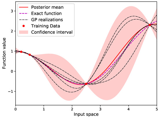
Figure 1.
Example of Gaussian process prediction and associated confidence interval.
An example of a 1D function and a GP built based on a dataset of data is represented in Figure 1. The confidence region for the prediction results from the associated GP standard deviation . At the observation locations the variance of the prediction is null if the data are not assumed noisy. The variance of the prediction grows as the distance from an existing data sample increases. GP surrogate model is appealing because it provides both the prediction of the model and its estimated uncertainty. This will be intensively used in the following of the paper to define an active learning strategy.
2.3. Quantile Estimation
The resulting surrogate model allows to define the output stochastic process as:
combining KL decomposition and Gaussian processes. It is possible to use this surrogate model to carry out uncertainty quantification studies instead of the exact computationally intensive function . For instance, it is possible to estimate an -quantile over the stochastic process surrogate model defined by:
For that, a Mont-Carlo simulation technique may be used by sampling according to as the computational cost is affordable using the surrogate model. Therefore, the quantile is estimated following these steps:
- Simulate samples according to
- Compute the empirical distribution function:
- Estimate the quantile by
However, due to the limited size of the training dataset used to build the surrogate model, the estimation of the quantile may present a large degree of uncertainty. In order to control the accuracy in the estimation of the quantile of using the surrogate model instead of the exact function, an active learning strategy is proposed in the following sections. It allows to follow an adaptive sampling strategy by adding relevant samples into the dataset in order to improve the accuracy of the estimation of the quantile while limiting the number of evaluations of the exact costly function .
3. Active Learning for Surrogate-Based Stochastic Process Quantile Estimation
In this section, an active learning strategy is proposed to improve the estimation of the quantile of a stochastic process defined over a mono-dimensional mesh domain. The active learning strategy consists of an adaptive sampling approach in order to add relevant samples into the input and output datasets for the quantile estimation. Firstly, considering the current dataset, an infill criterion is defined to quantify the possibility of improvement to reduce the uncertainty over the quantile estimation by reducing the uncertainty on the Gaussian processes involved in the prediction of the random variables of Karhunen–Loève (KL) decomposition. Secondly, the infill criterion is optimized through an auxiliary optimization problem to select the most interesting samples. These two elements are presented in the next sections.
3.1. Infill Criterion
The infill criterion for active learning is used to quantify the possibility of improvement of the quantile estimation given by a candidate sample to be added to the current dataset. The proposed infill criterion determines the confidence area associated to a quantile accounting for the uncertainty in the Gaussian processes involved in the KL decomposition. The proposed infill criterion calculation is summarized in Algorithm 1.
Let consider a potential candidate to be added to the current dataset . For each GP involved in the KL decomposition, the mean GP prediction is used to virtually extend the current dataset for the GPs. Therefore, the new input virtual dataset is and the GP output dataset is . Then, based on this dataset, the new “virtual” GPs are trained to update the hyperparameters , m and . Therefore, it is possible to define the resulting surrogate model for the stochastic process:
To estimate the influence of the virtual addition of the candidate sample into the dataset, Gaussian process trajectories are generated for each GP present in the KL decomposition. Then, quantiles of are estimated using:
and with a Monte-Carlo sampling (as explained in the previous section):
for . It results estimates of the quantile which may be used to define a confidence area associated to the quantile:
where and are upper and lower bounds on the quantile estimates in the set , for instance defined by a quantile of level and . The confidence area is computed over the mono-dimensional mesh domain (Figure 2). This confidence area translates the uncertainty in the quantile estimate due to the uncertainty in the Gaussian process given by the virtual current dataset which includes the candidate sample . It requires to evaluate times the surrogate model corresponding to the number of samples in the Monte-Carlo simulation for empirical quantile estimate times the number of GP trajectories sampled.
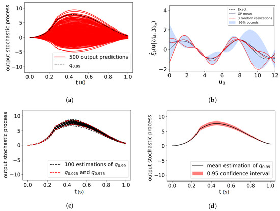
Figure 2.
(a) output stochastic process realizations and 99% quantile prediction, (b) the GPs involved in the surrogate model of the output stochastic process present uncertainty in the prediction and different GP realizations may be sampled (red curves), (c) for each GP realization, a quantile of the output stochastic process may be estimated (black dot lines), (d) based on the set of quantile estimations an confidence interval on the exact quantile may be estimated.
In order to improve the accuracy of the quantile estimate, a relevant candidate sample to be added to the current dataset is a sample that will reduce the uncertainty in the quantile estimate therefore that will reduce the confidence interval .
| Algorithm 1: Confidence interval area calculation for quantile estimation based on GP trajectories for a candidate sample |
Inputs: , , Initialization: , , , (1) Define new input and output “virtual” extended datasets and (2) Train the new “virtual” GPs based on and (3) Generate Gaussian process trajectories for the GPs in KL (4) for s = 1: do  end (5) Define the set of quantiles (6) Determine and as quantiles with and levels over the set . (7) Compute over the time mesh return |
3.2. Auxiliary Optimization Problem and Active Learning Process
In order to find the most relevant candidate sample to be added to the current dataset, an auxiliary optimization problem can be formulated:
where the objective function to be minimized corresponds to the confidence interval area calculation for quantile estimation as defined previously. The auxiliary optimization problem can be solved using an evolutionary algorithm (Covariance Matrix Adaptation—Evolution Strategy [28,29]). In cases of high-dimensional problems, gradient-based algorithms may be used (with analytical calculation thanks to the availability of the gradient of Gaussian-process) which scale better with the dimension [30].
Once the optimal solution has been found, the exact black-box model is evaluated. The input and output datasets are updated with the resulting stochastic process trajectory giving and . Then, based on these new input and output datasets a Karhunen–Loève decomposition is carried out and for each KL mode, a GP is built. The procedure of adding a new sample into the datasets is performed until a stopping criterion is met. The stopping criterion can be based either on the value of the confidence interval area or on a maximal number of exact black-box model evaluations. The proposed active learning strategy for quantile estimation refinement is summarized in Figure 3. In the following sections, the proposed active learning approach is applied on an analytical problem and a launch vehicle design problem.
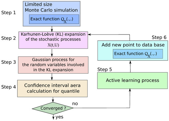
Figure 3.
Proposed active learning strategy for quantile estimation refinement for stochastic process defined over a mono-dimensional mesh domain.
4. Applications
4.1. Analytical Test Case
4.1.1. Test Case Description
To illustrate the proposed active learning approach, first an analytical test case is defined as follows (with a non-dimensional output):
where and . Moreover, with and , .
The objective is to estimate the quantile of the output stochastic process with the proposed active learning approach. The initial input and output datasets are defined by a Monte-Carlo simulation with . For each realization of the input uncertain variables, the exact mapping is evaluated to determine the output stochastic process realization . Then, 10 active learning iterations are carried out to enrich the input and output datasets in order to improve the estimation of the quantile with the surrogate model.
An illustration of 200 output stochastic process realizations and the exact quantile are given in Figure 4. Figure 5 presents the scaled KL modes for the output stochastic process.
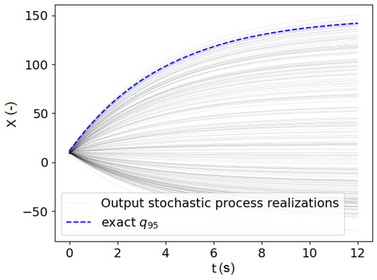
Figure 4.
Realizations of output stochastic process samples and exact quantile.
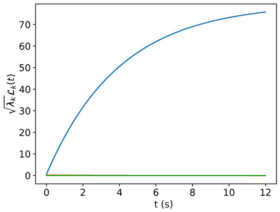
Figure 5.
13 scaled KL modes for the output stochastic process.
To evaluate the uncertainty on the quantile estimation, GP trajectories are sampled and is used to define the upper and lower bounds on the quantile estimates in the set .
To assess the adequate Karhunen–Loève decomposition, 1000 input variable samples are generated and the corresponding output stochastic process samples are estimated by running the model . These samples are used as validation samples .
The truncation level in Karhunen–Loève decomposition is a trade-off between the number of terms in the truncation and the accuracy of the resulting decomposition. The predictivity factor may be used to evaluate the accuracy of the KL expansion:
where is the number of validation samples, the exact validation sample and the KL expansion. The factor allows to evaluate the adequacy between the KL expansion prediction and the some validation samples resulting from the exact function evaluations. In the following, different number of KL modes are considered in the decomposition to analyze the influence of the truncation. For each level of truncation, the residual samples are determined by evaluating the difference between the validation samples and the KL predictions using Equation (4). The residual samples are illustrated in red in Figure 6 along with the validation samples (in blue). It can be seen in Figure 6, that by considering only 1 mode in the KL expansion, the residual samples are non negligible. However, as the number of modes increases, the residual samples become negligible and the KL expansion provides an accurate prediction.
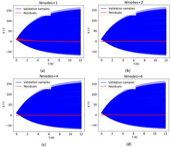
Figure 6.
Karhunen–Loève validation with respect to the number of modes: 1 (a), 2 (b), 4 (c), 6 (d).
Table 1 gives the factor according to the number of KL modes in the expansion. As expected from the Figure 6, with only 1 KL mode, the predictivity factor illustrates the poor accuracy of the KL decomposition. The predictivity factor converges to as the number of KL modes increases. The level of truncation is a compromise between the KL expansion accuracy and the number of KL modes (and therefore the number of Gaussian processes to use in the overall surrogate model). For the current test case, 4 KL modes are considered as it is a reasonable trade-off between the number of KL modes and the factor value.

Table 1.
Predictivity factor Q2 as a function of the number of KL modes.
4.1.2. Test Case Results
The proposed approach is repeated 10 times with different initial datasets and to evaluate the robustness of the proposed method to the initial datasets. For one representative repetition, the initial samples of the design experiment and the added samples by the active learning strategy are represented in Figure 7. As the infill process starts with a limited number of samples, the refinement strategy adds samples in the dataset to improve the quantile estimation. It can be seen that several (5 over 10) are added in the vicinity of the exact quantile.
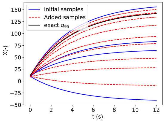
Figure 7.
Initial and added output stochastic process samples in the dataset.
Moreover, in Figure 8, the evolution of the estimated quantile with the surrogate model along with the iteration of the active learning process are presented. It can be seen that the first estimations of the quantile are far away from the exact and as the refinement strategy updates the surrogate model, the estimate quantile converges to the exact quantile thanks to a limited number of exact mapping evaluations. Therefore, the active learning process allows to estimate the quantile of the output stochastic process at an affordable computational cost.
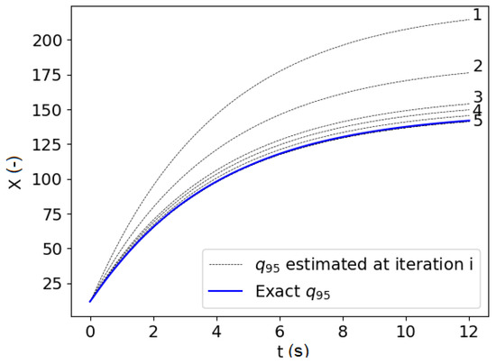
Figure 8.
Evolution of the estimated along the 10 active-learning iterations.
In addition, in Figure 9, the evolution of the quantile estimation and the confidence area are displayed before the refinement (left) and after the 10 active learning iterations (right). At the end of the refinement process, the estimated quantile converges to the exact quantile and the confidence area is tighten around the exact quantile.
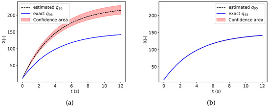
Figure 9.
Estimation of the quantile and its confidence area before refinement (a) and after 10 active-learning iterations (b).
Figure 10 presents the boxplots over the 10 repetitions corresponding to the evolution of the estimated quantile confidence area (left) and the root mean square error (RMSE) on the right with respect to the exact quantile. Both the confidence area and the RMSE decrease as the refinement strategy adds new relevant samples into the input and output datasets. The RMSE between the estimated quantile and the exact quantile converges to 0. Moreover, it can be noted that the proposed approach is robust to the different initial datasets. Therefore, with only 14 evaluations of the exact model (4 initial samples and 10 added with the refinement strategy) it is possible to accurately estimate the quantile while controlling the confidence in its estimation.
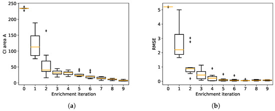
Figure 10.
Boxplots for 10 repetitions of the estimation of the quantile confidence area (a) and root mean square error (b) along the 10 active-learning iterations.
In order to illustrate the interest of the surrogate model-based approach for the estimation of the quantile, a Monte-Carlo simulation of the same number of samples (14 in the present case) may be performed to estimate the quantile. It is possible to determine the confidence area for the Monte-Carlo simulation as presented in Figure 11. For the same number of exact model evaluations , the estimated quantile is more accurate with the active learning approach compared to a Monte-Carlo estimation. It highlights the interest of surrogate-based estimation with a refinement strategy to estimate stochastic process quantile.
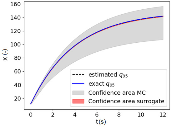
Figure 11.
Confidence area based on the surrogate model estimation and based on Monte Carlo (MC) with 14 evaluations of .
4.2. Launch Vehicle Design Problem
4.2.1. Test Case Description
This test case is derived from a launch vehicle design problem to estimate flight envelops considering modeling uncertainty. In the early design phase, in order to explore the design space at an affordable computational cost, low and medium fidelity models are used resulting in uncertainty in the estimated system performances. To evaluate the impact of the modeling uncertainty on the launch vehicle, uncertainty propagation is carried out. One objective is to estimate the launch vehicle flights envelopes that describe the possible trajectories considering the modeling uncertainty. The flight envelops are defined based on quantile estimation of the trajectory state variables such as altitude, velocity, flight path angle, etc.
In the current test case, the considered mission is to inject a payload of 10 tons into a 400 km circular equatorial orbit using a Two-Stage-To-Orbit (TSTO) vehicle. The launch vehicle has two stages: a first stage with nine rocket engines and a second stage with one rocket engine. All the engines use a combination of liquid oxydizer and rocket propellant (RP-1). The launch pad is located at the European spaceport at Kourou in French Guiana.
For one realization of the input uncertain modeling variables, the multidisciplinary analysis used to assess the vehicle performances consists in determining the optimal launch vehicle trajectory (optimal state variables) involving the solving of an optimal control problem. Therefore, uncertainty propagation is a challenge even in early design phases as it combines the computational cost of multidisciplinary analysis, uncertainty propagation and trajectory optimization.
In this test case, the surrogate-based model approach presented in the previous sections is carried out. It is assumed that the architecture of the launch vehicle is defined from a baseline and the objective is to assess the launch vehicle robustness to modeling uncertainty through the determination of flight envelops (extreme quantiles).
The input modeling uncertainties considered in this problem are gathered into an input uncertainty vector . These variables and their probability distributions are summarized in Table 2. These distributions have been assessed using expert knowledge. Four uncertainties are considered on the modeling of the propulsive performance: the specific impulse () of the first and second stages and the mass flow rate (). In addition, an uncertainty on dry masses is assumed using and to account for structural dry mass misknowledge in the early design phase. Eventually, for the aerodynamics model, it is assumed that the drag coefficient suffers from some uncertainty .
Table 2.
Probability distribution of the input uncertain random vector.
The launch vehicle performances are simulated through a multidisciplinary process that couples different disciplines: the structure, the aerodynamics, the propulsion and the trajectory (see Figure 12). All these disciplines are integrated into a Multidisciplinary Design Optimization process. The consistency between the coupling variables is ensured by a multidisciplinary analysis [31]. The implementation of the multidisciplinary process is done with the openMDAO framework [32]. The four disciplines are briefly introduced in the following paragraphs.
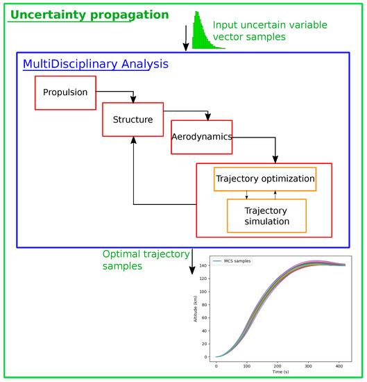
Figure 12.
Uncertainty propagation for launch vehicle design test case using multidisciplinary simulation.
Propulsion
The propulsion module is in charge of computing the rocket performances for the first and second stages. The propulsion module is based on the Chemical Equilibrium with Applications (CEA) model [33]. This code determines the rocket engine performances such as specific impulse and thrust based on different input characteristics (chamber pressure, oxydizer to fuel ratio, etc.). The model involves a thermochemical analysis of complex mixtures of propellants. For a rocket engine, it involves the combustion of injected gas in the combustion chamber and the hot gas expansion in the nozzle. CEA is suited for rocket engine calculations at the conceptual and preliminary design phases. It provides coupling variables (specific impulse, mass flow rate) that are transferred to the mass and sizing and the trajectory disciplines. To account for the modeling uncertainty, the nominal value of the estimated parameters by CEA is perturbed as presented in Table 2.
Structures
The structure discipline is in charge of estimating the dry mass of the two stages accounting for the coupling variables coming from the propulsion and trajectory disciplines. Mass Estimation Relationships (MERs) determined based on existing expandable launch vehicles are used [34] to estimate the masses of the different subsystems. All the different components of the launch vehicle (tanks, rocket engines, nozzle, avionics, electrical systems, thrust frame, interstage, etc.) are modeled. Their corresponding masses are estimated based on analytical relationships defined by the MERs. This discipline provides a fast estimation of the launch vehicle dry mass. To account for the fidelity level of the model, the dry mass of the first and second stages are assumed to be uncertain as presented in Table 2.
Aerodynamics
In order to evaluate the influence of the atmosphere during the launch vehicle flight, it is necessary to determine the aerodynamic loads that act on the launcher. The estimation of the aerodynamic forces for such a type of vehicles is difficult as it flows through very different phases (subsonic, transonic, supersonic and hypersonic). For early design phases, the aerodynamics model used in the multidisciplinary process is based on MISSILE datcom [35]. It is a semi-empirical code allowing to estimate the drag and lift coefficients as a function of the angle of attack and the Mach number, and the vehicle geometry. In the trajectory simulation, using an U.S. Standard Atmosphere models [36] and the aerodynamic coefficients, the discipline provides the aerodynamic loads given the current flight conditions. Uncertainty related to the estimation of the drag coefficient is assumed for this module as introduced in Table 2.
Trajectory
The trajectory discipline is in charge of optimizing the trajectory path in order to minimize the consumption of propellant during the flight. To simulate the flight of the launch vehicle, it is necessary to numerically integrate a system of ordinary differential equations that corresponds to the equations of motion according to the time. Different approaches exist to simulate and optimize the launch vehicle flight and in the multidisciplinary process, a pseudo-spectral method [37] is used in order to find the optimal control law. The control law consists of a parameterized pitch profile as a function of time. These parameters are optimized based on a Legendre–Gauss–Lobatto collocation technique [37] and DYMOS library [38].
The equations of motion that are considered involve five state variables:
with the angular velocity of the Earth, the longitude of the launch vehicle, the flight path angle, the position vector from the center of the Earth to the geometric center of the launch vehicle, the angle of attack, m the current launcher mass, q the mass flow rate, g the acceleration of gravity, L the lift force, D the drag force, the pitch angle, T the thrust force and v the velocity vector.
The trajectory is decomposed into five phases with appropriate guidance laws: lift-off, pitch-over maneuver, exponential decay, gravity turn and bi-linear tangent phase. Moreover, to represent the dynamics of the vehicle, the jettisoning of the first stage and payload fairing for the TSTO vehicle are included in the simulation. A Hohmann transfer ascent is implemented for the transfer before injection the payload on the circular target orbit.
4.2.2. Test Case Settings
The initial input and output datasets are defined by a Monte Carlo simulation with (see Figure 13). For each realization of the input uncertain variables, a multidisciplinary analysis is carried out with optimal control problem solving to determine the output stochastic process realization . The altitude as a function of time is considered as the quantity of interest resulting from the multidisciplinary analysis. In order to account for different trajectory durations depending on the input uncertain variables, the discretization is carried out with respect to a percent of flight from to . The objective of this test case is the determination of the quantile on the altitude as a function of percent of flight. For that purpose, considering the computational cost of one multidisciplinary analysis, 10 new samples are added into the database with the active learning algorithm to improve the estimation of the quantile over the stochastic process.
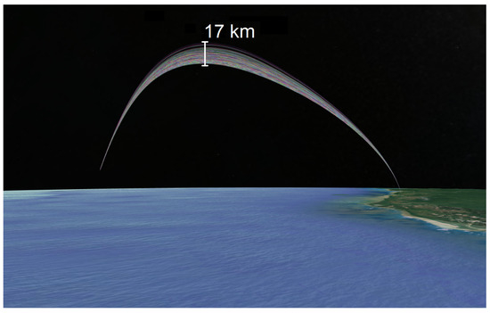
Figure 13.
Visualization of the launch vehicle ascent trajectories in 3D due to the uncertain input vector.
To evaluate the uncertainty on the quantile estimation, GP trajectories are sampled and is used to define the upper and lower bounds on the quantile estimates in the set . Figure 14 presents the scaled KL models for the centered altitude.
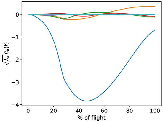
Figure 14.
Scaled KL models for the centered altitude.
The KL expansion validation is carried out using additional 800 validation samples. In that purpose, the exact multidisciplinary process is executed for the different input uncertain parameter values as defined in Table 2. The output samples are used for the validation.
Using the validation samples, it is possible to determine the residual samples as illustrated in red in Figure 15. The centered altitude samples are represented in blue. From Figure 15, it seems that with 2 modes in KL expansion, the obtained residual samples are non negligible meaning that the KL decomposition is not accurate enough. However, the increase of the number of modes leads to residual samples that becomes negligible validating the KL expansion accuracy.
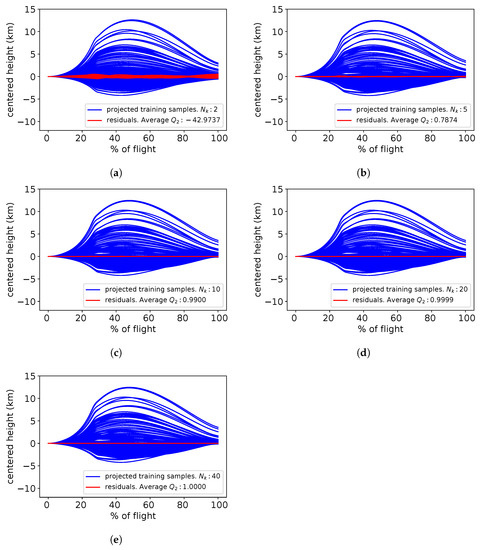
Figure 15.
Karhunen–Loève validation with respect to the number of modes: 2 (a), 5 (b), 10 (c), 20 (d) and 40 (e).
Table 3 gives the factor depending on the number of KL modes in the expansion. As expected from the Figure 15, by considering only 2 KL modes, the decomposition does not provide accurate results. As the number of modes in KL expansion increases, the prediction accuracy converges to . The level of truncation is a compromise between the number of nodes and the KL expansion accuracy. For the altitude variable, a number of 20 modes is a good trade-off between the number of GPs involves in the overall surrogate model and the factor.
Table 3.
Predictivity factor Q2 as a function of the number of KL modes.
4.2.3. Results Analysis and Discussion
The proposed approach is repeated 10 times with different initial dataset and to evaluate the robustness of the proposed method to the initial dataset. For one representative repetition, Figure 16 presents the initial (upper left) and final (lower left) output stochastic process samples corresponding to the launch vehicle altitude as a function of percent of flight. Moreover, the centered altitude process samples are illustrated on the figures of the right. It can be seen that the added samples (in dashed red) are in the higher region of the samples in order to refine the quantile of the altitude. Therefore, the refinement strategy selected appropriate new samples to improve the estimation of the quantile.
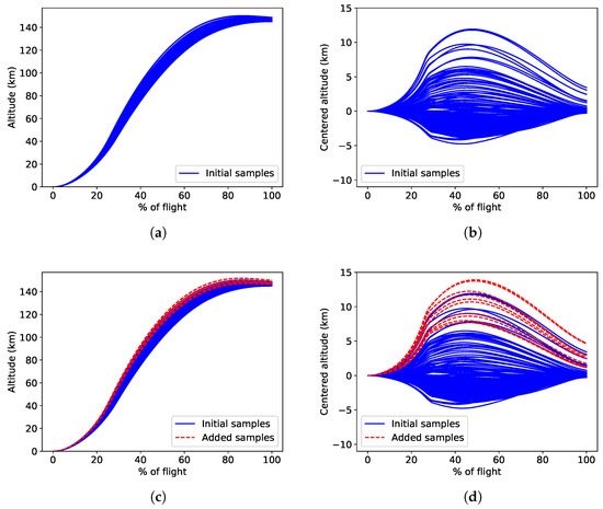
Figure 16.
Initial and final output stochastic process samples for the altitude (a,c) and the centered altitude (b,d).
For one representative repetition, Figure 17 presents the pairplot associated with the initial and added samples for the input uncertain variables in dimension 7. The added samples by the refinement strategy are selected in specific regions of the input uncertain variable domain. For instance, trajectories with higher altitude result from the uncertainty on the specific impulse of the 2nd stage that are above s offering higher rocket engine efficiency. Similarly, the negative uncertainty on the residual mass of the structures of stages 1 and 2 allows trajectories with higher altitude. Therefore, the active-learning strategy appropriately selects input uncertain variable realizations to be added to the surrogate model dataset to improve the quantile estimation.
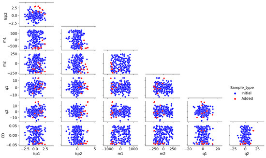
Figure 17.
Pairplot of the initial and added samples for the input uncertain variables.
For one representative repetition, the estimated quantile before and after refinement are presented in Figure 18. It can be seen that the uncertainty on the quantile estimation is reduced after the enrichment of the dataset and that the estimated quantile converged to the validation quantiles.
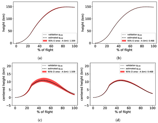
Figure 18.
Quantile estimation and confidence area with initial dataset (a,c) and after 10 active-learning-based enriched samples (b,d).
In Figure 19, boxplots of the 10 repetitions of the active-learning process are presented for the uncertainty on the quantile estimation (left) and the root mean square error (RMSE) of the obtained quantile compared to the validation quantile (right). The uncertainty on the quantile estimation is reduced along the addition of new sample in the dataset. Similarly, the RMSE compared to the validation quantile is also reduced as the number of selected samples by active-learning increase. These boxplots illustrate the efficiency of the proposed approach and its robustness with respect to the initial dataset.
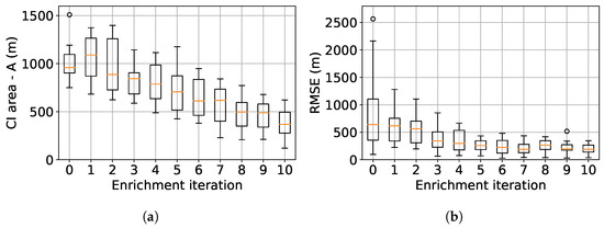
Figure 19.
Estimation of the quantile confidence area (a) and root mean square error (b) along the 10 active-learning iterations for 10 repetitions.
5. Conclusions
A methodology for uncertainty propagation though a computationally intensive black-box model with the output vector resulting in a discretization of a stochastic process has been proposed in this paper. The surrogate model approach combines Karhunen–Loève decomposition to carry out dimensionality reduction of the output stochastic process and Gaussian process to map the input uncertain variable realizations to the resulting output stochastic process samples. In order to control the accuracy of the quantile estimation, an active-learning strategy has been defined to carry out adaptive surrogate model refinement by evaluating the exact black-box model on relevant realizations of the input uncertain variable space. This strategy allows to estimate time-dependent extreme quantile in a limited number of computationally expensive code evaluations. In the involved examples. On the aerospace use case, only 10 enrichment iterations are needed to reduce the confidence area of the time-dependent extreme quantile to lower than 500 m. Furthermore, with the proposed approach, the Root Mean Square Error on the 99% quantile of the optimal altitude of the launcher decreases from 650 m before the infill down to 220 m after the addition of 10 new samples selected with the refinement strategy. In future works, an extension of the proposed approach for stochastic process defined over a multi-dimensional domain could be done by defining a new measure (integrated over the multi-dimensional domain) for the confidence associated to the quantile estimation.
Author Contributions
Conceptualization and methodology, L.B. and M.B.; investigation: J.-L.V.-Z. All authors have read and agreed to the published version of the manuscript.
Funding
This research received no external funding.
Acknowledgments
OpenTURNS library [39] has been used to carry out uncertainty quantification.
Conflicts of Interest
The authors declare no conflict of interest.
References
- Eldred, M. Recent advances in non-intrusive polynomial chaos and stochastic collocation methods for uncertainty analysis and design. In Proceedings of the 50th AIAA/ASME/ASCE/AHS/ASC Structures, Structural Dynamics, and Materials Conference 17th AIAA/ASME/AHS Adaptive Structures Conference 11th AIAA No, Palm Springs, CA, USA, 4–7 May 2009; p. 2274. [Google Scholar]
- Luthen, N.; Marelli, S.; Sudret, B. Sparse polynomial chaos expansions: Literature survey and benchmark. SIAM ASA J. Uncertain. Quantif. 2021, 9, 593–649. [Google Scholar] [CrossRef]
- Mara, T.A.; Becker, W.E. Polynomial chaos expansion for sensitivity analysis of model output with dependent inputs. Reliab. Eng. Syst. Saf. 2021, 214, 107795. [Google Scholar] [CrossRef]
- Zhang, J.; Yue, X.; Qiu, J.; Zhuo, L.; Zhu, J. Sparse polynomial chaos expansion based on Bregman-iterative greedy coordinate descent for global sensitivity analysis. Mech. Syst. Signal Process. 2021, 157, 107727. [Google Scholar] [CrossRef]
- Zhang, J.; Gong, W.; Yue, X.; Shi, M.; Chen, L. Efficient reliability analysis using prediction-oriented active sparse polynomial chaos expansion. Reliab. Eng. Syst. Saf. 2022, 228, 108749. [Google Scholar] [CrossRef]
- Rasmussen, C.E. Gaussian processes in machine learning. In Proceedings of the Summer School on Machine Learning, Tübingen, Germany, 4–16 August 2003; pp. 63–71. [Google Scholar]
- Schulz, E.; Speekenbrink, M.; Krause, A. A tutorial on Gaussian process regression: Modelling, exploring, and exploiting functions. J. Math. Psychol. 2018, 85, 1–16. [Google Scholar] [CrossRef]
- Binois, M.; Wycoff, N. A survey on high-dimensional Gaussian process modeling with application to Bayesian optimization. ACM Trans. Evol. Learn. Optim. 2022, 2, 1–26. [Google Scholar] [CrossRef]
- Capone, A.; Noske, G.; Umlauft, J.; Beckers, T.; Lederer, A.; Hirche, S. Localized active learning of Gaussian process state space models. In Proceedings of the Learning for Dynamics and Control, PMLR, Stanford, CA, USA, 23–24 June 2020; pp. 490–499. [Google Scholar]
- Zhao, G.; Dougherty, E.; Yoon, B.J.; Alexander, F.; Qian, X. Efficient active learning for Gaussian process classification by error reduction. Adv. Neural Inf. Process. Syst. 2021, 34, 9734–9746. [Google Scholar]
- Moustapha, M.; Marelli, S.; Sudret, B. Active learning for structural reliability: Survey, general framework and benchmark. Struct. Saf. 2022, 96, 102174. [Google Scholar] [CrossRef]
- Echard, B.; Gayton, N.; Lemaire, M. AK-MCS: An active learning reliability method combining Kriging and Monte Carlo simulation. Struct. Saf. 2011, 33, 145–154. [Google Scholar] [CrossRef]
- Echard, B.; Gayton, N.; Lemaire, M.; Relun, N. A combined importance sampling and kriging reliability method for small failure probabilities with time-demanding numerical models. Reliab. Eng. Syst. Saf. 2013, 111, 232–240. [Google Scholar] [CrossRef]
- Imani, M.; Ghoreishi, S.F. Bayesian optimization objective-based experimental design. In Proceedings of the 2020 American Control Conference (ACC), Denver, CO, USA, 1–3 July 2020; pp. 3405–3411. [Google Scholar]
- Picheny, V.; Wagner, T.; Ginsbourger, D. A benchmark of kriging-based infill criteria for noisy optimization. Struct. Multidiscip. Optim. 2013, 48, 607–626. [Google Scholar] [CrossRef]
- Janusevskis, J.; Le Riche, R. Simultaneous kriging-based estimation and optimization of mean response. J. Glob. Optim. 2013, 55, 313–336. [Google Scholar] [CrossRef]
- Iwazaki, S.; Inatsu, Y.; Takeuchi, I. Mean-variance analysis in Bayesian optimization under uncertainty. In Proceedings of the International Conference on Artificial Intelligence and Statistics, Virtual, 13–15 April 2021; pp. 973–981. [Google Scholar]
- Lyu, X.; Binois, M.; Ludkovski, M. Evaluating Gaussian process metamodels and sequential designs for noisy level set estimation. Stat. Comput. 2021, 31, 1–21. [Google Scholar] [CrossRef]
- Ghanem, R.G.; Spanos, P.D. Spectral stochastic finite-element formulation for reliability analysis. J. Eng. Mech. 1991, 117, 2351–2372. [Google Scholar] [CrossRef]
- Uribe, F.; Papaioannou, I.; Betz, W.; Straub, D. Bayesian inference of random fields represented with the Karhunen–Loève expansion. Comput. Methods Appl. Mech. Eng. 2020, 358, 112632. [Google Scholar] [CrossRef]
- Tipireddy, R.; Barajas-Solano, D.A.; Tartakovsky, A.M. Conditional Karhunen-Loeve expansion for uncertainty quantification and active learning in partial differential equation models. J. Comput. Phys. 2020, 418, 109604. [Google Scholar] [CrossRef]
- Brevault, L.; Balesdent, M. Uncertainty quantification for multidisciplinary launch vehicle design using model order reduction and spectral methods. Acta Astronaut. 2021, 187, 295–314. [Google Scholar] [CrossRef]
- Sudret, B.; Der Kiureghian, A. Stochastic Finite Element Methods and Reliability: A State-of-the-Art Report; Department of Civil and Environmental Engineering, University of California: Berkeley, CA, USA, 2000. [Google Scholar]
- Halko, N.; Martinsson, P.G.; Shkolnisky, Y.; Tygert, M. An algorithm for the principal component analysis of large data sets. SIAM J. Sci. Comput. 2011, 33, 2580–2594. [Google Scholar] [CrossRef]
- Brevault, L.; Balesdent, M.; Morio, J. Aerospace System Analysis and Optimization in Uncertainty; Springer: Berlin/Heidelberg, Germany, 2020. [Google Scholar]
- Matheron, G. Principles of geostatistics. Econ. Geol. 1963, 58, 1246–1266. [Google Scholar] [CrossRef]
- Sasena, M.J. Flexibility and Efficiency Enhancements for Constrained Global Design Optimization with Kriging Approximations; University of Michigan: Ann Arbor, MI, USA, 2002. [Google Scholar]
- Hansen, N.; Ostermeier, A. Adapting arbitrary normal mutation distributions in evolution strategies: The covariance matrix adaptation. In Proceedings of the IEEE International Conference on Evolutionary Computation, Nagoya, Japan, 20–22 May 1996; pp. 312–317. [Google Scholar]
- Dufossé, P.; Hansen, N. Augmented Lagrangian, penalty techniques and surrogate modeling for constrained optimization with CMA-ES. In Proceedings of the the Genetic and Evolutionary Computation Conference, Lille, France, 10–14 July 2021; pp. 519–527. [Google Scholar]
- Rana, S.; Li, C.; Gupta, S.; Nguyen, V.; Venkatesh, S. High dimensional Bayesian optimization with elastic Gaussian process. In Proceedings of the International Conference on Machine Learning, Sydney, Australia, 6–11 August 2017; pp. 2883–2891. [Google Scholar]
- Balesdent, M.; Bérend, N.; Dépincé, P.; Chriette, A. A survey of multidisciplinary design optimization methods in launch vehicle design. Struct. Multidiscip. Optim. 2012, 45, 619–642. [Google Scholar] [CrossRef]
- Gray, J.S.; Hwang, J.T.; Martins, J.R.; Moore, K.T.; Naylor, B.A. OpenMDAO: An open-source framework for multidisciplinary design, analysis, and optimization. Struct. Multidiscip. Optim. 2019, 59, 1075–1104. [Google Scholar] [CrossRef]
- McBride, B.J. Computer Program for Calculating and Fitting Thermodynamic Functions; National Aeronautics and Space Administration, Office of Management: Washington, DC, USA, 1992; Volume 1271. [Google Scholar]
- Castellini, F. Multidisciplinary Design Optimization for Expendable Launch Vehicles. Ph.D. Thesis, Politecnico di Milano, Milan, Italy, 2012. [Google Scholar]
- Blake, W.B. Missile Datcom: User’s Manual-1997 FORTRAN 90 Revision; Technical Report; Air Force Research Lab Wright-Patterson AFB OH Air Vehicles Directorate: Dayton, OH, USA, 1998. [Google Scholar]
- Krueger, A.J.; Minzner, R.A. A mid-latitude ozone model for the 1976 US Standard Atmosphere. J. Geophys. Res. 1976, 81, 4477–4481. [Google Scholar] [CrossRef]
- Betts, J.T. Survey of numerical methods for trajectory optimization. J. Guid. Control Dyn. 1998, 21, 193–207. [Google Scholar] [CrossRef]
- Falck, R.; Gray, J.S.; Ponnapalli, K.; Wright, T. dymos: A Python package for optimal control of multidisciplinary systems. J. Open Source Softw. 2021, 6, 2809. [Google Scholar] [CrossRef]
- Baudin, M.; Dutfoy, A.; Iooss, B.; Popelin, A.L. OpenTURNS: An industrial software for uncertainty quantification in simulation. arXiv 2015, arXiv:1501.05242. [Google Scholar]
Publisher’s Note: MDPI stays neutral with regard to jurisdictional claims in published maps and institutional affiliations. |
© 2022 by the authors. Licensee MDPI, Basel, Switzerland. This article is an open access article distributed under the terms and conditions of the Creative Commons Attribution (CC BY) license (https://creativecommons.org/licenses/by/4.0/).