Empirical Safety Stock Estimation Using GARCH Model, Historical Simulation, and Extreme Value Theory: A Comparative Study

Abstract

Safety stock (SS) is an appropriate tactic to deal with demand and supply uncertainty with the aim of preventing inventory shortages. In the literature, previous work on SS estimation assumes that the forecast error distributions (FED) are independent and identically distributed (i.i.d) following the normal distribution. In order to assess violations of this assumption, there are many solution methods in the recent literature that include the following: (1) Consider the FED as other distribution models, such as gamma distribution or log-normal distribution, etc. (2) Use the Generalized Auto-Regressive Conditional Heteroskedasticity (GARCH) model to consider the Heteroskedasticity phenomena, (3) Use the extreme value theory (EVT) to take into consideration the occurrence of extreme demands, etc. However, the performance of these methods is not guaranteed because there is an absence of comparative studies. Indeed, the estimation of SS is based on the approximation of quantiles of the FED. Such quantiles are related to the cycle service levels (CSL) that are important to achieve company goals. Accordingly, the aim of this research is to propose two combined empirical methods to determine the SS in a more robust fashion and compare them with traditional methods under different supply chain parameters. The first combined method, named Filtered Historical Simulation (FHS), consists of combining the GARCH model with the simulation method. The second combination named Conditional Extreme Value Theory (CEVT) is the GARCH model with EVT. To validate these proposed combined methods, the SS is also estimated using traditional methods, such as simple exponential smoothing (SES), simulation, and kernel density estimation (KDE). The methodology is illustrated with both simulation data and real case study data for different lead times. For the FED, two cases are studied: lognormal distribution and gamma distribution. The results show the superiority of the two proposed combination methods with respect to the tick loss function (TLF) for the different CSL targets and for shorter and longer lead times. Results are confirmed using the ANOVA test.

1. Introduction

1.1. Background and Research Motivation

In practice, there are two types of manufacturing processes: make-to-order (MTO) and make-to-stock (MTS). The MTO approach waits until a purchase order, work order, or sales order is created for a product before the advanced planning and scheduling process is involved. The MTS approach is based on forecasting customer demand to produce and manufacture goods. Forecasting is the basis for planning. For MTO, forecasting is not about demand, but about other parameters, such as lead time as in [1]. The lead time corresponds to the time that elapses between the placing of a supplier order and the delivery of the goods to the customer (this may be an individual or a point of sale). However, forecasting is considered the heart of the MTS approach to drive production systems based on material requirements planning. In the literature, there are many classifications of demand types [2,3]. However, little attention has been paid to measuring the uncertainty around those forecasts, although important applications, such as determining the safety stock (SS) and the reorder point in many replenishment policies, depend on estimating the uncertainty. Previous research on SS estimation can be classified into two groups. The first group assumes that forecast error distribution (FED) is normal, independent and identically distributed (i.i.d). The second group takes into consideration the heteroscedasticity phenomena. In the second group, some research proposes to apply SS estimation when extreme demands.

1.2. Literature Overview

1.2.1. Case When Forecast Errors Are Normal i.i.d

Traditional forecasting approaches are based on points forecasts, such as simple exponential smoothing (SES), AutoRegressive Mobile Average (ARMA), AutoRegressive Integrated Mobile Average (ARIMA), etc. These methods are vital especially for short- and medium-term applications and are also known for their simplicity in practice. However, how well it approximates the demand process has often not been sufficiently tested, due to the limited repertoire of forecasting model alternatives in software.

These methods mentioned above can be used if the demand process is perfectly identified, and therefore, the forecast errors are independent and identically distributed (i.i.d) in this case. These errors are usually assumed to be i.i.d as in Buffa [4], Fotopoulos et al. [5], Eppen and Martin [6], Potamianos et al. [7], Reichhart et al. [8], Gallego-García et al. [9], and Antic et al. [10]. However, it is reasonable to ask whether a correct identification of the process is possible given the complex relationships that drive the demand. Thereby testing the i.i.d assumptions on the errors is necessary. However, the forecast in the supply chain does not take into account the deviation from these assumptions and focuses on comparing different forecast error metrics, such as the mean absolute percentage error or the mean squared error, without analyzing the residual autocorrelation and deviations from the assumed statistical distribution [11]. According to [12] and [13], the stock control metrics, such as the cycle service level, inventory investments, and backorders can be under performance if the residuals are autocorrelated and distributed differently.

1.2.2. Case When Forecast Errors Are Not Normal i.i.d

Besides theoretical models assuming that the forecast errors are i.i.d, in practice this is not the case given the complexity of the supply chain; the use or at least the test of empirical approaches is crucial. When the deviation of the i.i.d assumptions is presented, other techniques, such as generalized autoregressive conditional heteroskedasticity (GARCH) [14], kernel density estimation (KDE) [15], and historical simulation [16] can be useful for forecasting the size of the uncertainty. Within a supply chain case study, Zhang and Kline [17] showed that ignoring temporal Heteroskedasticity can increase inventory costs by up to 30% when demand autocorrelation is highly positive. Syntetos and Boylan [18] examined the empirical performances of alternative forecasting methods by estimating the variability of the lead time forecast errors for improving the overall performance of the system. Trapero et al. [13] determined the variability of the lead time forecast error parametric models by applying GARCH models. Using simulated and real data, they showed that the forecast error standard deviation presented temporal autocorrelation for high lead times and that GARCH models yielded promising results.

In addition, usually, the demand distribution is assumed to be known despite this being not the case in practice, and future demand must be forecasted. Consequently, forecast errors are among the different factors required to calculate the SS [19], and the determination of their accurate standard deviation is particularly challenging. Some authors have criticized these assumptions, such as Boute et al. [20] and Charnes et al. [21] that can lead to mistakes in decisions regarding safety stocks and service objectives not being achieved. Trapero et al. [13,14,15,16,17,18,19,20,21,22] have used empirical methods based on non-parametric KDE and the parametric GARCH models for dimensioning the SS. They showed that the kernel density estimation technique gives better results in the case of shorter lead times because the no-normality is dominant. For longer lead times, conditional heteroscedasticity is more important and GARCH models are more suitable [22]. For continuous demand data, nonparametric approaches, such as simulation and KDE, take into account the nonnormality of forecast errors. These techniques can be used when the forecast error distribution is not known. The effectiveness of these methods has been shown, for example, in the works of Strijbosch and Heuts [23], Manary et al. [24] and Trapero et al. [13]. Manary et al. [24] tried to correct the impact of forecast bias, non-normal forecast errors, and heterogeneous forecast errors in the Intel company. The authors found SS reductions of approximately 15%. Strijbosch and Heuts [23] used an empirical dataset from the pharmaceutical industry to adjust statistical forecasts for ‘fast’ demand items. They provide information on the combined forecast and inventory performance of discretionary estimates.

1.2.3. Occurrence of Extreme Demands

Despite their research contributions, all these above-mentioned works did not take into consideration the presence of irregular data in the supply chain. This is very relevant for inventory management, where special events and promotions are common. The use of extreme value theory (EVT) improves and adjusts the SS computing for items that can record extraordinary demands. Within a supply chain case study, this approach has been reported as successful by Gallego et al. [25], Avanzi et al. [26], Bimpikis and Markakis [27], Biçer [28] and Fałdzinski et al. [29]. However, which method should be used if forecast errors possess both an auto-correlated standard deviation, an unknown density function, and an irregular demand process?

To solve these questions, several combination methods have been proposed in the literature, and in practice, it turns out that the combination of two or more forecasting methods gives the best predictive performance compared to the predictions given by a single method [30].

1.3. Objective of the Study

According to the above literature overview, previous work on SS estimation assumes that the FED are normal i.i.d In order to assess violations of this assumption, there are many solution methods in the recent literature, such as considering the FED as a gamma distribution or log-normal distribution, using the GARCH model to consider the Heteroskedasticity phenomena, and using EVT to take into consideration the occurrence of extreme demands. However, the performance of these methods is not guaranteed because there is an absence of comparative studies. Consequently, the final objective of this research can be summarized by the following primary research question. How can we improve the SS estimation methods to simultaneously consider the Heteroskedasticity phenomena and the occurrence of extreme demands?

This work proposes to estimate SS using two methods mentioned above, which are also largely applied in finance and insurance domains to estimate Value at Risk which is defined as the quantile of the studied distribution for a given confidence level. The first method consists of combining simulation and GARCH methods, named filtered historical simulation (FHS), while the second one consists of combining EVT with the GARCH model, named conditional extreme value theory (CEVT). The choice to combine EVT and simulation with GARCH can be justified also by the success of these methods in providing a sufficient estimation of VaR in the risk measurement context. For each method, in the first step GARCH parameters we extract standardized residuals, and then, in the second step, we apply either EVT or historical simulation to residual series obtained from the GARCH model. This two-step procedure is different from traditional combination techniques, such as that applied by Trapero et al. [22] to combine kernel estimation and GARCH methods. To the best of our knowledge, this is the first work to evaluate SS using these two methods and that compares their performance against traditional methods assuming a demand that follows the AR process with nonnormal distributions for residuals. We follow relatively similar methodology as Trapero et al. [22] with some divergence, especially in the case study and in the choice of distribution parameters. Trapero et al. [22] used an optimization framework to determine the optimal weight of each method used in combination. On the contrary, in our paper, the combination is based on each of the simulation and EVT methods applied to standardized residuals obtained from the GARCH model. Furthermore, the combination of GARCH models are very useful in the estimation methods for other areas, such as stock price volatility estimation [31], value at risk estimation [32], crude oil price volatility estimation [33], etc.

The novelty of this research is about the proposition of new combined methods for SS estimation in the case when forecast errors are not normal i.i.d and to simultaneously consider the Heteroskedasticity phenomena and the occurrence of extreme demands. To the best of the authors’ knowledge, this is the first time a quantile combination using FHS and CEVT has been used to calculate the SS. To validate the superiority of the proposed methods, both simulation and real data from a case study are applied. In the simulation, three cases are studied as follows. Case 1: when the forecast error follows a normal distribution, Case 2: when the forecasting error follows a lognormal distribution, and Case 3: when the forecasting error follows a gamma distribution. Moreover, to validate the statistical significance of the obtained simulation results, the one-way ANOVA technique is applied.

2. Materials and Methods

2.1. Theoretical Safety Stock Estimation

Safety stock can be calculated using different approaches. The most appropriate method depends on the circumstances of an organization. As the stock-out cost can be very difficult to estimate in practice, calculating the SS based on an ordering policy that does not require knowledge of cost is recommended. Customer service is frequently used in the literature.

The safety stock dimensioning depends on the levels of demand uncertainty and the corresponding forecast errors when the forecast errors are assumed independent and identically distributed (i.i.d). In other words, the forecast errors follow a normal distribution with zero mean and constant variance; safety stock is computed using Equation (1).

$$\mathrm{SS}={\mathrm{k}\mathsf{\sigma }}_{\mathrm{L}},$$

(1)

where:

${\mathsf{\sigma }}_{\mathrm{L}}$: standard deviation of the forecasting error for a certain lead time LT,

k: the safety factor with a chosen cycle service level (CSL). It is estimated using Equation (2).

$$\mathrm{k}={\mathsf{\varphi }}^{-1}\left(\mathrm{CSL}\right),$$

(2)

ϕ(.) is the standard normal cumulative distribution function.

The lead time (LT) is considered to be known and constant. In this case, the problem is how to calculate ${\mathsf{\sigma }}_{\mathrm{L}}$. An initial theoretical approach is considered in which the standard deviation of the forecasting error ${\mathsf{\sigma }}_{\mathrm{L}}$is estimated on the basis of the demand forecasting model.

${\mathsf{\sigma }}_{\mathrm{L}}$is estimated using the standard deviation ${\mathsf{\sigma }}_1$ which is based on forecasting the mean squared error (MSE).

$${\mathsf{\sigma }}_1=\sqrt{\mathrm{MSE}},$$

(3)

The cumulative variance forecasting error is calculated and then the safety stock is computed using the theoretical well-known formulas as mentioned in Equation (4).

$$\mathrm{SS}=\mathrm{k}.{\mathsf{\sigma }}_1.\sqrt{\mathrm{LT}},$$

(4)

Equation (4) is used when the forecast errors are independent and do not vary for longer forecast horizons [34]. However, when demand can be expressed by a single exponential smoothing (SES) model method [35]. The safety stock will be expressed in Equation (5).

$$\mathrm{SS}=\mathrm{k}.{\mathsf{\sigma }}_1.\sqrt{\mathrm{LT}}\sqrt{1+{\mathsf{\alpha }}^{\prime }\left(\mathrm{LT}-1\right)+\frac{1}{6}{{\mathsf{\alpha }}^{\prime }}^2\left(\mathrm{LT}-1\right)\left(2\mathrm{LT}-1\right)},$$

(5)

where:

${\mathsf{\alpha }}^{\prime }$: is the SES parameter that is constant and varies between 0 and 1.

Equation (4) of the safety stock is the most useful in the literature, although Equation (5) offers an accurate relationship. One of the major drawbacks of the theoretical approach is that it disregards the fact that the forecast errors are not i.i.d in reality. In addition, the true model of each item is not found and also the choice of the forecasting error model cannot be under the control of the firm. To overcome the i.i.d problem of the forecast errors and the problem when the distribution of forecast errors is unknown, a second empirical approach is considered in which neither the point forecast model nor its parameters must be known. This is mainly beneficial in practice, especially when such information is not provided to users.

2.2. Empirical Safety Stock Estimation

Different empirical approaches can be utilized to calculate the SS. Some of these approaches suppose the normality distribution of forecast errors but take into account that the forecast error variance varies over time, i.e., regard the heteroscedasticity phenomena. In this case, the SS can be calculated using Equation (6).

$$\mathrm{SS}=\mathrm{k}.{\mathsf{\sigma }}_{\mathrm{L}}=\mathrm{k}.\sqrt{\frac{{{\displaystyle \sum }}_{\mathrm{t}=1}^{\mathrm{n}}{\left({\mathsf{\epsilon }}_{\mathrm{L},\mathrm{t}}-{\overline{\mathsf{\epsilon }}}_{\mathrm{L}}\right)}^2}{\mathrm{n}}}$$

(6)

where ${\mathsf{\epsilon }}_{\mathrm{L},\mathrm{t}}$ is the forecast error for a certain lead time L, expressed in Equation (7)

$${\mathsf{\epsilon }}_{\mathrm{L},\mathrm{t}}={\mathrm{y}}_{\mathrm{L}}-{\mathrm{F}}_{\mathrm{L}}={{\displaystyle \sum }}_{\mathrm{h}=1}^{\mathrm{L}}\left({\mathrm{y}}_{\mathrm{t}+\mathrm{h}}-{\mathrm{F}}_{\mathrm{t}+\mathrm{h}}\right)$$

(7)

${\overline{\mathsf{\epsilon }}}_{\mathrm{L}}$ is the average error during the lead time

${\mathrm{y}}_{\mathrm{L}}$ and ${\mathrm{F}}_{\mathrm{L}}$ are, respectively, the actual value and the forecast value during the lead time.

Some others of these approaches take into account the non-normality of forecast errors (the distribution of forecast errors is unknown) due to, for example, the promotional periods, and complexity of markets; the safety stock is computed as the quantile (denoted by Q) of the distribution of forecast errors at the probability defined by the CSL.

2.2.1. Simple Exponential Smoothing (SES)

According to Gardner [36], SES is the most widely used forecasting method in the short term. It is an easy to understand and efficient procedure to use when the underlying demand model is composed of level and random components. Even when the underlying demand process is more complicated, exponential smoothing can be used as part of an update procedure.

SES is a t + 1 forecasting method. It is used with trendless time series. The principle of this method of calculation consists of giving greater importance to the last observations made. Therefore, SES is used as expressed in Equation (8).

$${\mathrm{MSE}}_{\mathrm{L},\mathrm{t}+1}=\mathsf{\gamma }{\left({\mathsf{\epsilon }}_{\mathrm{L},\mathrm{t}}\right)}^2+\left(1-\mathsf{\gamma }\right){\mathrm{MSE}}_{\mathrm{L},\mathrm{t}}$$

(8)

where:

$\sqrt{{\mathrm{MSE}}_{\mathrm{L},\mathrm{t}+1}}$: is the forecast for ${\mathsf{\sigma }}_{\mathrm{L}}$ at time t + 1.

${\mathsf{\epsilon }}_{\mathrm{L},\mathrm{t}}$: the cumulative forecast error during the lead time.

$\mathsf{\gamma }$: a constant smoothing parameter. Its value lies between 0 and 1.

Following the proposal of Morgan [37], the value of $\mathsf{\gamma }$ and the initial value of Equation (8) are optimized by minimizing the mean squared errors.

2.2.2. Historical Simulation (HS)

Historical simulation is used as the most popular and efficient method [38]. The main characteristics of this method are that it is relatively simple to set up, it does not provide any assumption about the form of distribution and its dependence on the availability of data and the sample size.

While predicting the future implies inherent uncertainty, a point forecast can be very useful to quickly describe the general expected path with less complexity. The first step before dimensioning SS is computing the point forecast. Then, this value is used with the forecast error for the quantile forecasting approaches. The SES method is used in this work to find the point forecasts [36] and is formulated as mentioned in Equation (9). To initialize this method, the value of the smoothing parameter ${\mathsf{\alpha }}^{\prime }$ and the initial value of Equation (9) is optimized via minimizing the in-sample MSE.

$${\mathrm{F}}_{\mathrm{t}+\mathrm{h}}={\mathsf{\alpha }}^{\prime }{\mathrm{y}}_{\mathrm{t}}+\left(1-{\mathsf{\alpha }}^{\prime }\right){\mathrm{F}}_{\mathrm{t}}$$

(9)

where

$0<{\mathsf{\alpha }}^{\prime }<1,$

h is the forecasting horizon.

Note, that the lead time demand forecast F_L is expressed as mentioned in Equation (10).

$${\mathrm{F}}_{\mathrm{L}}={{\displaystyle \sum }}_{\mathrm{h}=1}^{\mathrm{L}}{\mathrm{F}}_{\mathrm{t}+\mathrm{h}}=\mathrm{L}.{\mathrm{F}}_{\mathrm{t}+1}.$$

(10)

Then, the empirical quantile method is a simple approach to estimating SS. It is based on the empirical distribution of historical data on the lead time forecast errors as expressed according to Equation (11).

$$\mathrm{SS}=\mathrm{Q}\left(\mathrm{CSL}\right)-\mathrm{point}\mathrm{forecast}$$

(11)

where $\mathrm{Q}\left(\mathrm{CSL}\right)$ is the quantile of empirical distribution at CSL.

2.2.3. Kernel Density Estimation (KDE)

The Kernel density estimation (KDE) method expressed the probability density function f (x) of forecast errors during the lead time. It does not provide any assumption regarding the form of data distribution. On every data point xi, we place a kernel smoothing function K. The KDE is expressed in Equation (12).

$$\hat{\mathrm{f}}\left(\mathrm{x}\right)=\frac{1}{\mathrm{N}}{\displaystyle \sum }_{\mathrm{i}=1}^{\mathrm{N}}\mathrm{K}\left(\mathrm{x}-{\mathrm{x}}_{\mathrm{i}}\right)$$

(12)

We use h to control the bandwidth of $\hat{\mathrm{f}}\left(\mathrm{x}\right)$ by writing Equation (13) as proposed by Silverman [16].

$$\hat{\mathrm{f}}\left(\mathrm{x}\right)=\frac{1}{\mathrm{Nh}}{\displaystyle \sum }_{\mathrm{i}=1}^{\mathrm{N}}\mathrm{K}\left(\frac{\mathrm{x}-{\mathrm{x}}_{\mathrm{i}}}{\mathrm{h}}\right)$$

(13)

Where N is the sample size. The kernel function K is typically: Everywhere non-negative: $\mathrm{K}\left(\mathrm{x}\right)\ge 0$ for every x, Symmetric: $\mathrm{K}\left(\mathrm{x}\right)=\mathrm{K}\left(-\mathrm{x}\right)$ for every x and Decreasing: ${\mathrm{K}}^{\prime }\left(\mathrm{x}\right)\le 0$ for every $\mathrm{x}>0$.

The Epanechnikov kernel, which means optimal kernel function, is given by Equation (14).

$$K_e\left(\mathrm{t}\right)=\{\begin{array}{c}\frac{3}{4\sqrt{5}}\left(1-\frac{{\mathrm{t}}^2}{5}\right),\mathrm{if}-\sqrt{5}\le \mathrm{t}\le \sqrt{5}\\ 0,\mathrm{Else}\end{array}$$

(14)

For a Gaussian kernel, the following optimal bandwidth [39] is usually chosen as shown in Equation (15).

$${\mathrm{h}}_{\mathrm{opt}}=0.9{\mathrm{AN}}^{-(1/5)}$$

(15)

where A is an adaptive estimate of the spread that is computed using Equation (16).

A = min (standard deviation, interquantile range/1.34)

(16)

The empirical quantile $\mathrm{Q}\left(\mathrm{CSL}\right)$ is estimated basis on the empirical distribution fitted by the kernel approach on the forecast errors during lead time.

2.2.4. GARCH Models

To cope with the time-variation of lead time forecast errors’ standard deviation the generalized autoregressive conditional heteroscedastic (GARCH) models can be used for capturing the ‘fat’ tails and heteroscedasticity [40].

The expression of GARCH (p, q) models is given by the conditional variance of the forecast error at time t + 1. This variance is given by Equation (17).

$${\mathsf{\sigma }}_{\mathrm{t}+1}^2=\mathsf{\omega }+{{\displaystyle \sum }}_{\mathrm{i}=1}^{\mathrm{p}}{\mathrm{a}}_{\mathrm{i}}{\mathsf{\epsilon }}_{\mathrm{t}}^2+{{\displaystyle \sum }}_{\mathrm{j}=1}^{\mathrm{q}}{\mathsf{\beta }}_{\mathrm{j}}{\mathsf{\sigma }}_{\mathrm{t}}^2$$

(17)

where q is the lagged conditional variance terms (${\mathsf{\sigma }}_{\mathrm{t}}^2$) and p is the lagged squared error terms (${\mathsf{\epsilon }}_{\mathrm{t}}^2$).

We can notice that the SES method in Equation (9) is a particular case of the GARCH model when p = q = 1. Knowing that a GARCH (1,1) is given by Equation (18).

$${\mathsf{\sigma }}_{\mathrm{t}+1}^2=\mathsf{\omega }+{\mathrm{a}}_1{\mathsf{\epsilon }}_{\mathrm{t}}^2+{\mathsf{\beta }}_1{\mathsf{\sigma }}_{\mathrm{t}}^2$$

(18)

then replacing the one-step-ahead forecasting error with the cumulative lead time forecast error, Equation (11) can be rewritten as Equation (19)

$${\mathsf{\sigma }}_{\mathrm{L},\mathrm{t}+1}^2={\mathsf{\omega }}^{\prime }+{\mathrm{a}}_1^{\prime }{\mathsf{\epsilon }}_{\mathrm{L},\mathrm{t}}^2+{\mathsf{\beta }}_1^{\prime }{\mathsf{\sigma }}_{\mathrm{L},\mathrm{t}}^2$$

(19)

Then, the safety stock is computed using the Equation (20)

$$\mathrm{SS}=\hat{\mathrm{D}}+\mathrm{Q}\left(\mathrm{CSL}\right){\hat{\mathsf{\sigma }}}_{\mathrm{L}}-\mathrm{point}\mathrm{forecast}$$

(20)

where

$\widehat{D}$ is demand forecast for a certain lead time L,

${\hat{\mathsf{\sigma }}}_{\mathrm{L}}$ is the standard deviation of the forecast error for a certain lead time L,

$\mathrm{Q}\left(\mathrm{CSL}\right)$is the quantile of standard normal distribution at CSL and the point forecast is given in Equation (9).

2.2.5. Extreme Value Theory (EVT)

This method is a prevailing tool to study the tail behavior of the demand distribution by taking into account the occurrence of abnormal and extreme events due to the complexity of the markets, customers, promotions, and the economic situation. The use of this theory improves and adjusts the SS computing for items that can record extraordinary demands.

In this method, the maximums and minimums of the data converge to the generalized extreme value (GEV) distribution or the generalized Pareto distribution (GPD). Two traditional approaches are introduced in the literature: the Block maxima method (BM) and the Peack over threshold (POT) method. We are interested in the POT method, in the rest of this work, which considers as extreme each observation beyond a certain threshold u. In this case, several observations of a turbulent period, which records extreme demands, are retained as extremes, while any observation of a calm period is considered as extremes. The determination of u is problematic, and various approaches are used in the literature, such as the mean excess function (MEF) and the hill plot. The reader can consult Fisher and Tippet [41] for more detailed discussions and several examples on the use of hill plots to approximate the threshold value u.

The expression for quantiles associated with a given CSL is described in Equation (21).

$$\mathrm{Q}\left(\mathrm{CSL}\right)=\mathrm{u}+\frac{\hat{\mathsf{\beta }}}{\hat{\mathsf{\xi }}}\left({\left(\frac{\mathrm{n}}{{\mathrm{N}}_{\mathrm{u}}}\mathrm{p}\right)}^{-\mathsf{\xi }}-1\right)$$

(21)

where

n is the total sample size,

$\hat{\mathsf{\beta }}$ is the scale factor,

${\mathrm{N}}_{\mathrm{u}}$ is the number of observations beyond threshold u,

$\mathsf{\xi }$ is the tail index of the GPD distribution that can be positive or negative or null,

$\mathrm{p}=1-\mathrm{C}\mathrm{S}\mathrm{L}$.

We can then deduce the safety stock level using Equation (11).

2.3. Proposed Combined Safety Stock Estimation

Two method combinations are studied in this research. The first one named Filtered Historical Simulation (FHS) consists of combining the GARCH model with the Historical Simulation (HS) method. The second combination named Conditional Extreme Value Theory (CEVT) is about the GARCH model with Extreme Value Theory (EVT).

2.3.1. Filtered Historical Simulation (FHS)

The power of this method is that can adapt to the presence of heteroscedasticity phenomena and the asymmetry of the empirical distribution contrary to the traditional simulation method. The application of this method is given by modeling the data by the most appropriate GARCH (parametric) specification, deriving standardized residuals and applying the historical simulation method (non-parametric) for computing the quantile. Then, the safety stock is obtained using Equation (20) where the $\mathrm{Q}\left(\mathrm{CSL}\right)$ is the quantile of standardized residuals obtained from the GARCH model.

2.3.2. Conditional Extreme Value Theory (CEVT)

To take into account the heteroscedasticity phenomena and occurrence of extreme demands simultaneously, we can combine the GARCH model and Extreme Value Theory following the same two-step estimation procedure proposed by McNeil and Frey [42]. Such method is known under the name conditional EVT or GARCH-EVT:

Step 1: Fit a GARCH family model to the demand data by quasi-maximum likelihood estimation. We assume that innovations are normally distributed when maximizing the log-likelihood function. Once the parameters are estimated, we can extract the standardized residuals to check the adequacy of the GARCH modeling.

Step 2: We apply EVT to the standardized residual computing in step 1 to model the tail of innovations. In this work, we fix a certain threshold and we retain every innovation over this threshold and consider it extreme (POT Method). The threshold is determined under the condition that only 10% of innovations are greater than it, i.e., we consider the quantile of innovation distribution of order 90%. Then, we estimate the quantiles of innovations as presented in Equation (21) where the $\mathrm{Q}\left(\mathrm{CSL}\right)$ is not applied to demand series but applied to standardized residual series.

Finally, we deduce safety stock for various levels using Equation (20) with the $\mathrm{Q}\left(\mathrm{CSL}\right)$ being the quantile of standardized residuals obtained from the GARCH model.

2.4. Performance Metrics of Safety Stock Estimation Method

2.4.1. Inventory Performance Metrics

The different forecasting approaches are evaluated and compared through the different curves described in the results section. In this work, the two variables considered in the curves are inventory investment and backorders. A single-period newsvendor problem inspired by the literature is considered an empirical study. The inventory investment is calculated as follows: we calculate first the prediction interval of each item, then the average of the upper bound of the prediction interval per item and via items correspond to the inventory investment. The backorder units are calculated by the difference between the actual sales and quantile forecasts. Indeed, if such a difference is positive then it corresponds to backorder units. These units are summed for each item and then we calculate the average backorder units of all items.

2.4.2. Tick loss Function (TLF)

To facilitate the comparison between different approaches to safety stock calculation, we need to add other performance metrics in addition to inventory investment and backorders. According to Trapero et al. [22], the solution is given by the tick loss function (TLF) which is utilized in economic performance. The function associated averages the asymmetric costs of under- and over-prediction. The ‘‘best’’ approach is that which has the minimum loss value. We combine these mentioned approaches to minimize the TLF. The expression of TLF is given in Equation (22).

$${\mathrm{TL}}_{\mathsf{\alpha }}\left({\mathrm{y}}_{\mathrm{t}},{\mathrm{F}}_{\mathrm{t}}\right)=\{\begin{array}{c}\mathsf{\alpha }\left|{\mathrm{y}}_{\mathrm{t}}-{\mathrm{F}}_{\mathrm{t}}\right| \mathrm{if} {\mathrm{F}}_{\mathrm{t}}\le {\mathrm{y}}_{\mathrm{t}}\\ \left(1-\mathsf{\alpha }\right)\left|{\mathrm{y}}_{\mathrm{t}}-{\mathrm{F}}_{\mathrm{t}}\right|\mathrm{if} {\mathrm{F}}_{\mathrm{t}}\ge {\mathrm{y}}_{\mathrm{t}}\end{array}$$

(22)

where

${\mathrm{y}}_{\mathrm{t}}$ is the actual value at time t,

${\mathrm{F}}_{\mathrm{t}}$ is the forecast value at time t,

The parameter $\mathsf{\alpha }$ varies between 0 and 1 and any $\mathsf{\alpha }$-quantile of the predictive distribution is an optimal point forecast. In this work, the target quantile is given by the CSL.

2.5. Safety Stock Estimation Methods Implementation

In this study, we set the target CSL to 85%, 90%, 95% and 99%. The dataset is divided as follows: The first part of the data present 30% of data and are employed to establish the point demand forecast by calculating foremost both the exponential smoothing parameter and its initial value. The second part is used to predict the KDE, GARCH, FHS and CEVT methods. The last part is employed for testing the quantile forecasts of the methods considered.

The Epanechnikov kernel smoothing function is used for the KDE; the bandwidth of the appropriate value that is optimal for normal distribution densities is defined [43]. The GARCH (1,1) parameters are estimated based on the maximum Likelihood estimation method.

The analysis was conducted using R. The R package ‘rugarch’ is used to estimate GARCH parameters and to extract standardized residuals while the ‘evir’ package is used to perform the estimation of the POT model applied to filtered data. We use the ‘forecasts’ package equally to calculate the exponential smoothing parameter and the ‘kde1d’ Package to provide an efficient implementation of univariate local polynomial kernel density estimators.

3. Simulation Results

To evaluate the performance of the proposed combined methods, we performed a simulation (Monte Carlo) with 100 repetitions. The length of each repetition was fixed to 700 realizations. We choose 700 observations to guarantee that the number of extrema becomes sufficient to fit and estimate the parameters of GPD distribution. The simulation experiences were made with an AR (1) demand process while the point forecasting is an SES method following the same procedure as in McNeil and Frey [41]. The choice of the AR (1) demand process is explained by the fact that is widely used to describe the series in datasets (see for instance Ali et al. [44] and Trapero et al. [45].

In this study, we have compared these different empirical methods mentioned in Section 2 for computing safety stocks assuming foremost that the forecast error ε_t is i.i.d normally distributed with zero mean and a variance of σ². We found that the CEVT method always gives good results for most values of quantiles followed by the FHS and GARCH methods. We show in the first following subsection the overview results of this case. Thus, this work is interested to confirm these results when the forecast errors follow a non-normal distribution (log-normal and gamma distribution). The log-normal distribution is used to model demand when products are subject to promotional periods characterized by observed demand that is higher than the baseline demand. The gamma distribution and Beta distribution have previously been used in the literature ([46,47,48,49,50]) to assess violations of the normality assumption. Following Keaton [46], the gamma distribution is an especially effective choice because it is flexible and has non-negative values as the real demand. Burgin [47] justify the applicability of the gamma distribution and show that a particular advantage of the gamma distribution is that it may be used to deal with fixed lead times and that it can be extended to situations where the lead time is a random variable.

Detailed results are provided in Supplementary Tables S1, S2, S3 and S4. Table S1: contains the Tick loss values corresponding to Lead Time 1 week, when forecasting errors follow a Log-Normal distribution, and ϕ range from −0.90 to ϕ = 0.90. Table S2 contains the Tick loss values corresponding to Lead Time 4 weeks, when forecasting errors follow a Log-Normal distribution, and ϕ range from −0.90 to ϕ = 0.90. Table S3 contains the Tick loss values corresponding to Lead Time 1 week, when forecasting errors follow a gamma distribution, and ϕ range from −0.90 to ϕ = 0.90. Table S4 contains the Tick loss values corresponding to Lead Time 4 weeks, when forecasting errors follow a gamma distribution, and ϕ range from −0.90 to ϕ = 0.90.

3.1. Case wWhen Forecasting Error Follows A Normal Distribution

We assumed that the demand at time t follows an AR (1) process as mentioned in Equation (23).

$${\mathrm{D}}_{\mathrm{t}}=\mathsf{\mu }+\varphi {\mathrm{D}}_{\mathrm{t}-1}+{\mathsf{\epsilon }}_{\mathrm{t}}$$

(23)

where µ is a positive constant, ϕ is the autoregressive parameter and ε_t is Gaussian i.i.d with null mean and a standard deviation of 5 while ϕ was allowed to vary between −0.9 and 0.9. The value of µ used for the simulation is 150.

The TLF on the retained sample averaged over 100 replicates and then over the quantiles which include the following values namely 85%, 90%, 95% and 99%, versus the autoregressive parameter ϕ assumed to vary between -0.90 and 0.90 are made.

Table 1. Tick loss function values corresponding to ϕ = 0.70 and ϕ = −0.70 when forecasting errors follow a normal distribution.

Safety Stock Estimation Method	LT = 1 Week	ϕ = 0.70				ϕ = −0.70
		CSL				CSL
		85%	90%	95%	99%	85%	90%	95%	99%
Simple methods	SES	3.51	2.74	1.73	0.55	2.32	1.75	1.03	0.26
	HS	2.31	1.74	1.03	0.22	2.32	1.74	1.02	0.26
	KDE	2.34	1.76	1.05	0.28	2.32	1.75	1.03	0.27
	GARCH	2.15	1.59	0.93	0.24	2.17	1.60 1	0.93	0.24
Combined methods	FHS	2.15	1.59	0.93	0.24	2.16 1	1.61	0.93	0.24
	CEVT	2.05 1	1.55 1	0.89 1	0.22 1	2.22	1.62	0.92 1	0.22 1
	LT= 4 Weeks	ϕ = 0.70				ϕ = −0.70
		CSL				CSL
		85%	90%	95%	99%	85%	90%	95%	99%
Simple methods	SES	8.97	6.82	4.11	1.17	2.46	1.85	1.09	0.28
	HS	7.71	5.79	3.42	0.94	2.44	1.85	1.09	0.29
	KDE	7.86	5.94	3.54	0.95	2.46	1.86	1.11	0.30
	GARCH	7.63	5.70	3.32	0.85 1	2.42	1.82	1.06	0.27
Combined methods	FHS	7.66	5.71	3.32	0.90	2.42	1.83	1.07	0.28
	CEVT	7.06 1	5.11 1	3.10 1	0.95	2.21 1	1.65 1	0.95 1	0.24 1

¹ Minimum values of Tick loss shown in bold.

gives the tick loss values of each SS measurement method for the four CSL levels and for a lead time of one week and four weeks assuming demand that follows the AR (1) process with normal distribution and ϕ= −0.70 or ϕ = 0.70. Values in the blood indicate the minimum tick loss for a given CSL level. For example, the value of tick loss in the case of ϕ = 0.70 and lead time of one week is 2.05 at an 85% level when we apply the CEVT method. This value decreases to 0.22 when CSL is 99%. We choose the lead time of four weeks to imply a minimum value of tick loss of 7.06 for the 95% level and 0.95 for 99% level. We can remark the sensitivity of tick loss to various factors, such as the value of ϕ, lead time, and CSL level. It appears that the CEVT method provides the most performance in the majority of cases followed by the FHS method and GARCH. This points out that there is an autocorrelation in the estimating of error variability that can be explained by the fact that the prediction model does not correspond exactly to the demand generation process. Traditional methods cannot provide good results by comparison with GARCH-based methods. The SES method offers the worst performance in terms of TLF.

3.2. Case When Forecasting Error Follow A Log-Normal Distribution

Let D_t be the demand at time t that follows an AR (1) process as mentioned in Equation (23), where µ is a positive constant, ϕ is the autoregressive parameter and ε_t is i.i.d but is not normally distributed. We have added a log-normal noise with a mean of 0.9 and variance of 1.4, while ϕ was allowed to vary between −0.9 and 0.9.

The TLFs on the retained sample averaged over 100 replicates; the quantiles which include the following values namely 85%, 90%, 95% and 99%, versus the autoregressive parameter ϕ are assumed to vary between -0.9 and 0.9 and are shown in Figure 1 and Figure 2.

Figure 1 includes the case where the Lead time (LT) is one and Figure 2 includes the case where the LT is four weeks. When the case of LT is one week, the CEVT method (purple line) provided a low value for average tick loss for some values of the ϕ parameter. For the other values of ϕ where CEVT is not the best method we find in this case, the method of FHS (yellow line) gives better results followed by the GARCH (blue line) method. This proved the best performance of the GARCH model and Extreme Value Theory (CEVT) and secondly of the GARCH and simulation method (FHS) method which is explained by their nature to capture the deviation from the normality assumption. When the case of LT is four weeks and for negative values of ϕ it appears that CEVT is the best method except when ϕ = −0.4, the FHS gives a minimum of tick loss followed by the GARCH method. For positive values of ϕ, we find that the CEVT method is the best for some values of the autoregressive parameter otherwise the FHS takes its place followed by the GARCH method. The SES method offers the worst performance in terms of tick loss followed by the KDE and simulation methods.

Figure 1 and Figure 2 indicate the overall results. Nevertheless, the performance of the GARCH-based methods can be shown by choosing particular values of the autoregressive parameter ϕ and plotting the tradeoff curves and tick loss value for each quantile of interest.

Table 2. Tick loss function values corresponding to ϕ = 0.70 and ϕ = −0.70 when forecasting errors follow a lognormal distribution.

Safety Stock Estimation Method	LT = 1 Week	ϕ = 0.70				ϕ = −0.70
		CSL				CSL
		85%	90%	95%	99%	85%	90%	95%	99%
Simple methods	SES	3.68	3.02	2.12	1.01	2.88	2.38	1.66	0.76
	HS	3.12	2.63	1.87	0.74	2.65 1	2.24	1.61	0.70
	KDE	3.14	2.66	1.90	0.80	2.67	2.26	1.64	0.74
	GARCH	2.46	2.05	1.46	0.69	2.66	2.20	1.64	0.71
Combined methods	FHS	2.42 1	1.99 1	1.44 1	0.62 1	2.67	2.08 1	1.63	0.72
	CEVT	3.10	2.60	1.84	0.64	3.53	2.99	1.58 1	0.74
	LT = 4 Weeks	ϕ = 0.70				ϕ = −0.70
		CSL				CSL
		85%	90%	95%	99%	85%	90%	95%	99%
Simple methods	SES	12.00	9.77	6.68	2.98	3.38	2.83	2.03	1.04
	HS	10.55	8.77	6.13	2.30	3.23	2.77 1	2.01	0.92
	KDE	10.62	8.86	6.32	2.60	3.28	2.81	2.11	0.96
	GARCH	10.36	8.44	5.70	2.29	3.38	2.80	1.97	0.92
Combined methods	FHS	10.20 1	8.40 1	5.65 1	1.90 1	3.27	2.78	1.97	0.77
	CEVT	11.42	9.69	6.27	2.53	3.08 1	2.78	1.97 1	0.48 1

¹ Minimum values of Tick loss shown in bold.

gives the tick loss values of each safety stock measurement method for the four CSL levels and for an LT of one week and four weeks assuming demand that follow the AR (1) process with log-normal distribution and ϕ = 0.70 or ϕ = −0.70.

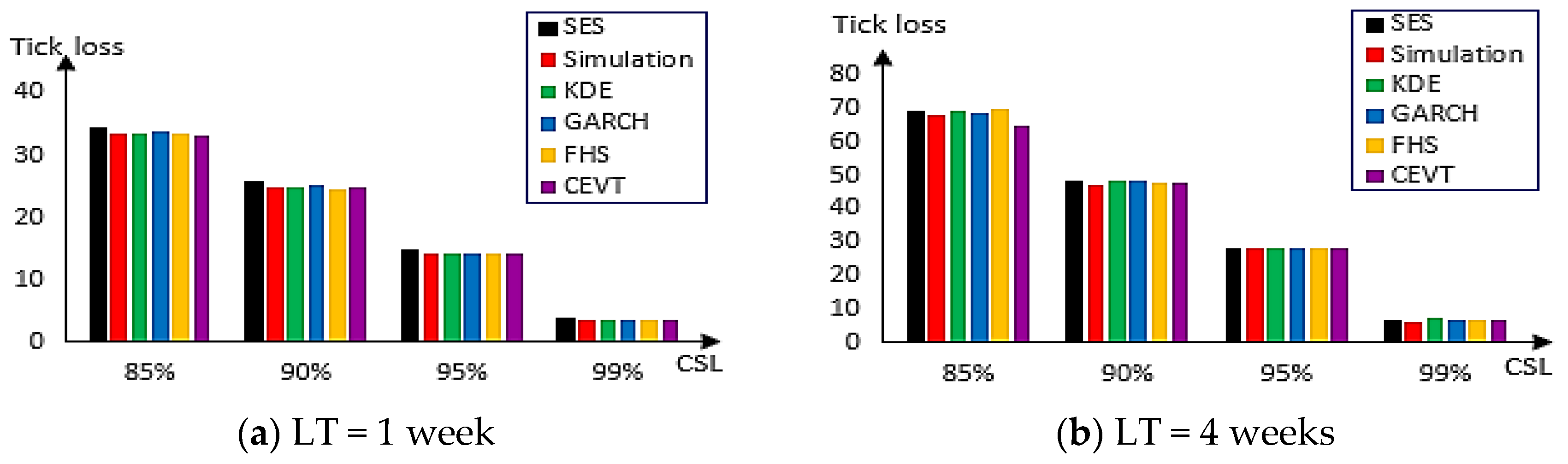
Values in blood in Table 2 indicate the minimum tick loss for a given CSL. The tick loss values in the table are also plotted in Figure 3. For example, the value of tick loss in the case of ϕ = −0.70 and an LT of four weeks is 3.08 at an 85% level when we apply the CEVT method. This value decreases to 0.48 when the CSL becomes at 99%. Choosing an LT of one week implies a minimum value of tick loss of 1.58 only for the 95% level. In the same case and at a 90% level, the FHS method gives better results. Additionally, in the case of ϕ = 0.70 and LT of one week, FHS is more important compared with other methods given a minimum of tick loss for all CSL. This result is the same for four weeks. It appears that the FHS method provides the most performance in the majority of cases followed by the CEVT method and GARCH. Traditional methods cannot provide good results in comparison to GARCH-based methods.

Figure 3 shows the tick loss values in the case of log-normal distribution for ϕ = 0.70 (on the left) and ϕ = −0.70 (on the right) and lead times of one week (upper panel) and four weeks (lower panel). We can remark for the four panels when the CEVT provides a higher tick loss value we find that the FHS provides the lowest loss, followed by the GARCH method and vice versa.

Figure 4 shows the tradeoff curves in the case of lognormal distribution for ϕ = 0.70 (on the left) and ϕ = −0.70 (on the right) and lead times of one week (upper panel) and four weeks (lower panel). This figure plotted the backorders versus inventory investment. Each curve for each panel contained four specific points corresponding to the four targets CSL (85%, 90%, 95% and 99%).

It is difficult to determine the best method since for instance in the left upper panel and at the 99% level, the CEVT provides a lower level of backorders but gives a higher inventory investment. Contrary, the GARCH method gives a lower inventory investment but provides a higher level of backorders. Despite these conflicts, it is clear that the GARCH-based methods and especially GARCH always give good results for all panels and almost all CSL targets.

3.3. Case When Forecasting Error Follow to Gamma Distribution

Let D_t be the demand at time t that follows an AR (1) process as mentioned in Equation (23). Where µ is a positive constant, ϕ is the autoregressive parameter and ε_t is followed by the Gamma distribution with parameters alpha= 0.4 and beta = 0.07 while ϕ was allowed to vary between −0.9 and 0.9.

The TLFs on the retained sample averaged over 100 replicates and then over the quantiles which include the following values namely 85%, 90%, 95% and 99%, versus the autoregressive parameter ϕ, assumed to vary between -0.9 and 0.9, are shown in Figure 5 and Figure 6. Figure 5 includes the case when the LT is one and Figure 6 shows the case when the LT is four weeks.

When the case of LT is one week and for negative values of ϕ, the CEVT method provided a low value for average tick loss except in ϕ = −0.4 and ϕ = −0.2, the FHS method gives a minimum tick loss. For positive values of ϕ, the CEVT method gives a lower loss for only three values of ϕ and for the remaining values, the FHS is the best method followed by GARCH. We can remark that the GARCH method gives good results especially for negative or positive high values of ϕ. This proved the best performance of the combination of GARCH-based methods. When the case of LT is four weeks, for negative values of ϕ it appears that CEVT is the best method except when ϕ = −0.4. The other methods including the traditional and combined approaches give nearly the same minimum of tick loss. For positive values of ϕ, we find that the CEVT method is the best for values of the autoregressive parameter otherwise the FHS takes its place followed by the GARCH method. The SES method offers the worst performance in terms of tick loss followed by KDE and simulation methods.

Figure 5 and Figure 6 indicate the overall results. Nevertheless, the performance of the GARCH-based methods can be shown by choosing particular values of the autoregressive parameter ϕ and plotting the tradeoff curves and tick loss value for each quantile of interest.

Table 3. Tick loss values corresponding to ϕ = 0.70 and ϕ = −0.70 when forecasting errors follow a gamma distribution.

Safety Stock Estimation Method	LT= 1 Week	ϕ = 0.70				ϕ = −0.70
		CSL				CSL
		0.85	0.90	0.95	0.99	0.85	0.90	0.95	0.99
Simple methods	SES	3.87	3.10	2.07	0.84	3.10	2.50	1.66	0.64
	HS	3.37	2.73	1.79	0.57	3.04	2.48	1.65	0.54
	KDE	3.42	2.77	1.83	0.59	3.05	2.50	1.67	0.56
	GARCH	2.75	2.25	1.54 1	0.65	2.97	2.42	1.63	0.67
Combined methods	FHS	2.74 1	2.24 1	1.54 1	0.55	2.89	2.38	1.64	0.56
	CEVT	3.76	2.95	1.84	0.521	2.51 1	2.04 1	1.48 1	0.44 1
	LT= 4 Weeks	ϕ = 0.70				ϕ = −0.70
		CSL				CSL
		0.85	0.90	0.95	0.99	0.85	0.90	0.95	0.99
Simple methods	SES	11.88	12.27	6.17	2.38	3.49	2.83	1.92	0.79
	HS	10.93	9.43	5.62	1.82	3.48	2.83	1.87	0.62
	KDE	11.14	8.73	5.73	1.84	3.50	2.85	1.90	0.67
	GARCH	10.66 1	8.88	5.34	1.80	3.46	2.79	1.85	0.70
Combined methods	FHS	10.72	8.40 1	5.28 1	1.58	3.47	2.80	1.82	0.56 1
	CEVT	12.27	8.41	5.56	1.37 1	2.79 1	2.32 1	1.62 1	0.59

¹ Minimum values of Tick loss shown in bold.

gives the tick loss values of each safety stock measurement method for the four CSL levels and for an LT of one week and four weeks assuming demand that follow the AR (1) process with a gamma distribution and ϕ = 0.70 or ϕ = −0.70. Values in blood indicate the minimum tick loss for a given CSL.

The tick loss values of such a table are also plotted in Figure 7. In the case of ϕ = −0.70 and LT of one week it appears that the CEVT method provides the most performance in all targets CSL followed by the FHS method. For example, the value of tick loss is 2.51 at an 85% level when we apply the CEVT method. This value decreases to 0.44 when CSL becomes at 99%. For an LT of four weeks, the CEVT method gives a lower loss except at the 99% level where the FHS method provides the minimum value of tick loss. Additionally, in the case of ϕ = 0.70 and LT of one week, FHS is more important compared with other methods given a minimum of tick loss for almost all CSL except at the 99% level where the CEVT is better. Contrary to LT of four weeks, FHS is more suitable only in 90% and 95% levels. The GARCH and CEVT methods are more appropriate, respectively, when the CSL is equal to 85% and 99%. Traditional methods (SES, simulation and KDE) cannot provide good results by comparison with GARCH-based methods.

Figure 7 shows the tick loss values in the case of gamma distribution for ϕ = 0.70 (on the left) and ϕ = −0.70 (on the right) and lead times of one week (upper panel) and four weeks (lower panel). We can remark for the four panels when the CEVT provides a higher tick loss value we find that the FHS provides the lowest loss, followed by the GARCH method and vice versa. Figure 8 shows the tradeoff curves in the case of gamma distribution for ϕ = 0.70 (on the left) and ϕ = −0.70 (on the right) and lead times of one week (upper panel) and four weeks (lower panel).

Figure 7 plotted the backorders versus inventory investment. Each curve for each panel contained four specific points corresponding to the four targets CSL (85%, 90%, 95% and 99%). We can see in the case of ϕ = −0.70 that the CEVT method gives good results in terms of inventory investment and backorders for CSL targets 85%, 90% and 95%. The 99% level provides a lower level of backorders but does not give the minimum inventory investment. Therefore, it is difficult to determine the best method. We can also see in the case of ϕ = 0.70 that the GARCH method provides results with the FHS, notably for lead times of one week.

3.4. Case Study Results

3.4.1. Case Study Data Set

The dataset used in this work comes from a major manufacturer that specializes in the production of cardboard packaging and cases. It specifies the manufacture of personalized corrugated cardboard packaging as well as the transformation of paper and the manufacture of cardboard boxes. The data represent a series of demands with 775 weekly observations for a cardboard product used for the packaging of bakery goods and on which there is the printing and design of this product as well as the name of the company requesting this product.

As in the case of the simulated data we used the SES method for the point forecasts. The use of this method in an industrial context is strongly recommended [51,52].

Note, according to

Table 4. Descriptive statistics and preliminary tests.

Min	Max	Median	Mean	Skewness	Kurtosis	Jarque Bera Test	Augmented Dickey Fuller Test	Q (12)	Q2 (12)
0	928.9	463.7	458	−0.003	45.365	790.3	−9.0986	30.47	28.707

the real demand is not normally distributed and presents a phenomenon of autocorrelation of orders 1 and 2, hence the interest in modeling by an ARMA-GARCH model. Based on the Akaike Information Criterion (AIC) the more adequate model is AR(1) GARCH(1,1). Estimate parameters of this model are given in

Table 5. ARMA-GARCH parameters estimation.

Parameter	Estimate	Std. Error	t-Value	p-Value
mu	458.45	6.31	72.64	0.000
ar1	0.17	0.04	4.76	0.000
omega	31.56	77.84	0.41	0.685
alpha1	0.00	0.00	0.81	0.420
beta1	1.00	0.00	1688.02	0.000
Q (12)	6.68			0.878
Q2 (12)	18.42			0.110
ARCH test	19.15			0.090
Log Likelihood	−4962.29
AIC	12.82
BIC	12.85
Shibata	12.82
H-Q	12.83

.

3.4.2. Case Study Safety Stock Estimation

Two simulations are performed with the real data for one and four weeks of lead times. Figure 9 shows the weekly demand for the item over time. Figure 10 presents the tick loss values of each method for real demand that follows the ARMA-GARCH model for one week (on the right) and for four weeks (on the left). When the case of LT is one week, the CEVT approach reduced the loss to a 85% level. This is valid when the LT is four weeks. For the other CSL, almost all methods give the same value of tick loss.

Figure 11 shows the backorders of each method for real demand that follows the ARMA-GARCH model for one week (on the left) and for four weeks (on the right).

In the case of shorter LT and at an 85% level we can remark that the GARCH method provides a lower level of inventory investment but gives higher backorders. Contrary the CEVT method gives lower backorders but provides a higher level of inventory investment. The result of the FHS method is the compromise between such methods. When the CSL is equal to 90% the combination of FHS and CEVT approaches provide almost the same result. Concerning backorders, the two techniques outperform the GARCH method but in terms of inventory investment this approach works better. At the 95% level, the GARCH-based methods yield the lowest backorders and inventory investment with CEVT improving on FHS and GARCH slightly in terms of backorders. We can see for CSL= 99% that the GARCH approach outperforms slightly the rest of the methods.

In the case of longer lead times for CSL= 85% the CEVT performs better regarding backorders and there is a slight difference regarding inventory investment in favor of FHS followed by the GARCH technique. Note, that these three approaches always give better results for 90% and 95% CSL with a slight difference regarding backorders or inventory investment. The combination technique FHS attains the best results with the lowest level of backorders and lowest inventory investment for CSL= 99%. Generally, such a figure indicates the good performance of GARCH-based methods compared with the traditional approaches for every CSL target for shorter lead times except for the 99% level where GARCH performs better. For longer lead times that achievement remains except for the 99% level where FHS yields the best results. These results obtained with real data match those with the simulated data carried out in the previous section. That coincidence is in the sense that the GARCH method and their combination with the simulation and EVT always perform better.

4. Discussion

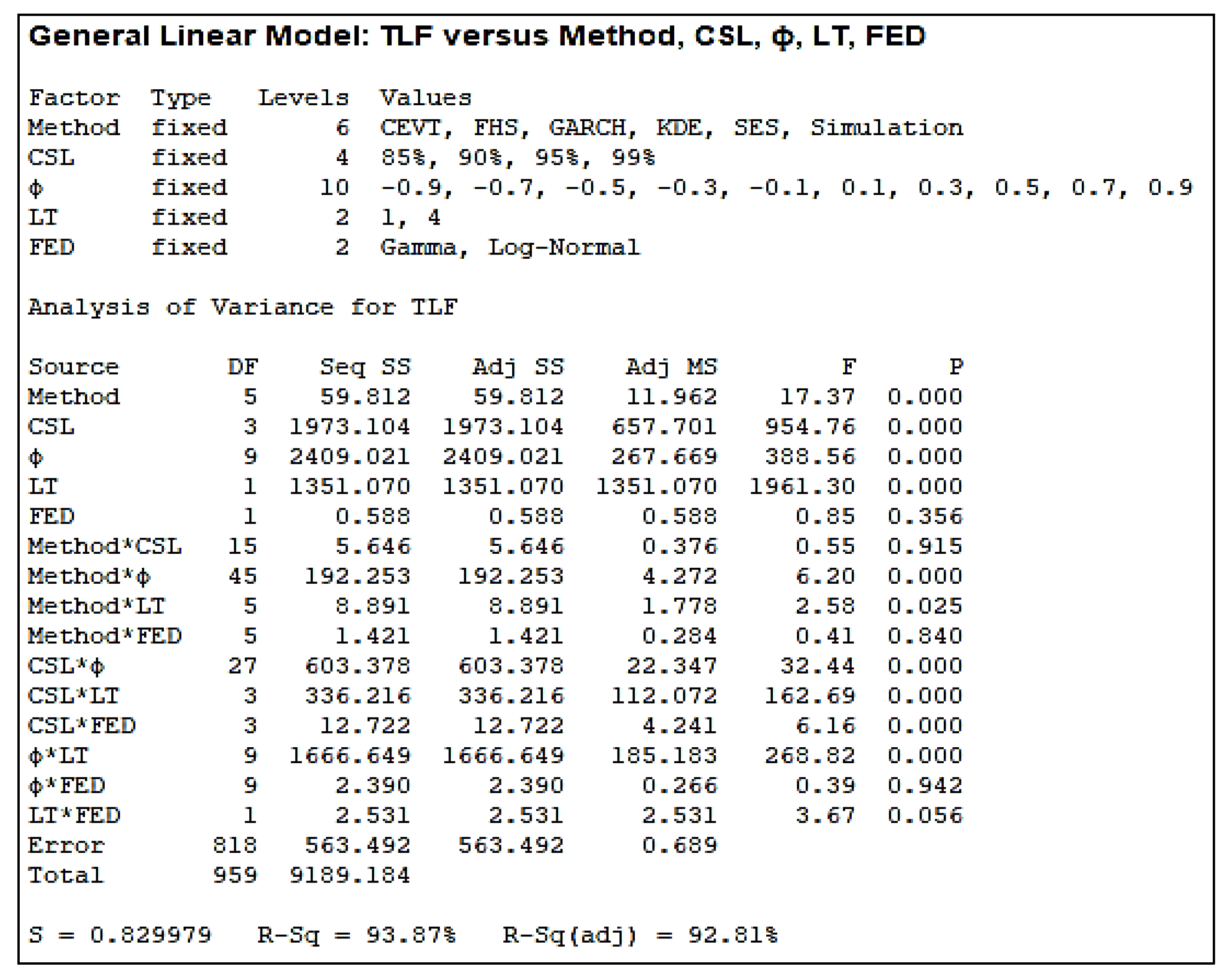
To validate the superiority of the two proposed SS estimation methods, it is necessary to study the significance of the difference between the tick loss of each combined SS estimation method. For these reasons, the Analysis of Variance (ANOVA) technique is used to test the difference between the six studied methods means and between other factor means, such as the value of CSL with four levels (85%, 90%, 95%, and 99%), the value of ϕ with 10 levels (range from −0.90 to 0.90), LT with two levels (1 week, and 4 weeks), and FED with two levels (gamma distribution, log normal distribution).

To perform the ANOVA test, a full design of experiments with 960 runs is used with only one response (output): TLF and five input factors: Method (six levels), CSL (four levels), ϕ (10 levels), LT (two levels), and FED (two levels). Using Minitab Software, the ANOVA results are presented in Figure 12.

For each input factor, this test has two hypotheses (H₀: all means are the same, vs. H₁: not all the means are equal). To the right of the ANOVA table (Figure 12), under the column headed P, is a p-value. If the p-value is less than 0.05 then H₀ is rejected and the result provides sufficient evidence to conclude that the TLF is not all the same for all levels.

Through the ANOVA test, we can conclude that the used estimation method, the CSL, the autoregressive parameter (ϕ) and the lead time have a significant influence on TLF and consequently on the estimation of the safety stock. However, the forecast error distribution (FED) has no influence on the decision since the related p-value = 0.356 is higher than 0.05. This indicates that the TLFs are the same when the forecast errors follow a log-normal or a gamma distribution.

Although an ANOVA test does tell whether different groups or treatments were statistically significantly different, it does not tell (1) if that difference is practically significant and (2) it does not use a grouping method that can help separate the differences in performance between each of the different safety stock estimation methods used in this manuscript. Consequently, it is necessary to look at confidence intervals or run post hoc tests to determine that. However, in this research, pair-wise comparison between methods is not applied because the ANOVA test used in this manuscript is not one-way ANOVA. Extending the current research in this direction is one of our interesting perspectives.

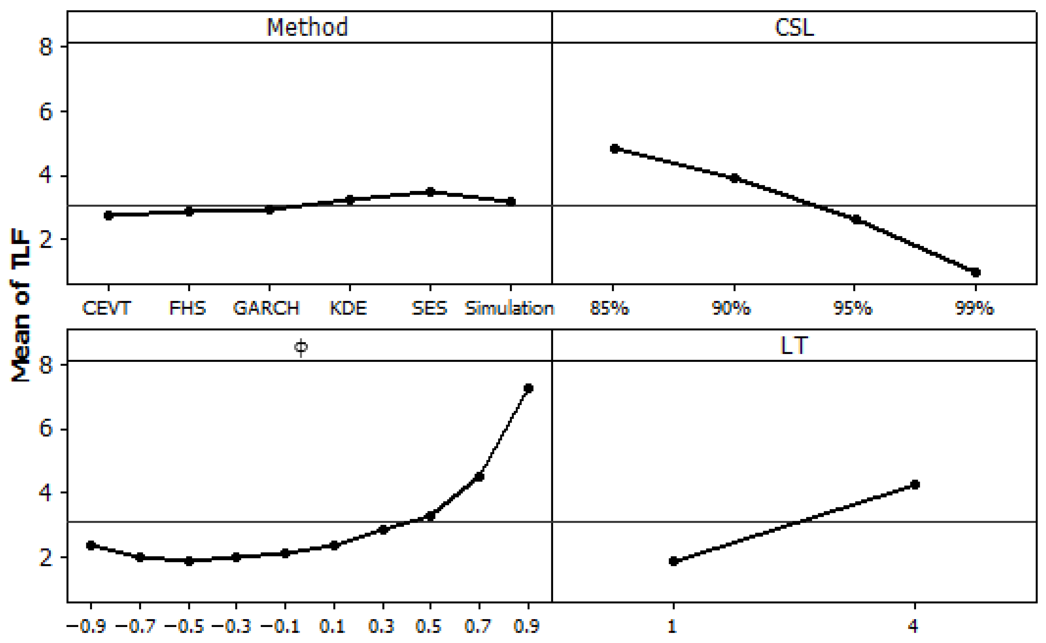
ANOVA results (effect and interactions) and the main effect plot shown in Figure 13, validate the simulation results and confirm that the two combined method for safety stock estimation FHS and CEV gives the minimum tick loss values and they are better than the classical methods, such as the SES method, Simulation method, KDE method, and GARCH method. We can verify also in Figure 13, that the tick loss is better when CLS = 99% and when the lead time is equal to one week. The value of TLF decreases when the CSL increases from 85% to 99% levels. This indicates that gradually as the target probability of no stock out over the LT (CSL) increases the actual demands and the forecast demands values are getting closer, and therefore, the TLF values decrease. Similarly, as the LT increases, the uncertainty increases implying the growth of TLF values. We can conclude also that when the autoregressive parameter increases implying a strong autocorrelation between the past and actual demands, the TLF values also increases.

5. Conclusions

The safety stock estimation needs forecast error uncertainty measurement. Deviation to the normal distribution and i.i.d assumptions lead to a problem in practice. Although certain forecasting models have analytical expressions for the variance over lead time, again retaining the same assumptions, these typically are not considered in practice.

The use of empirical approaches, as developed in this research, overcomes these limitations, as the assumptions are relaxed and the error distribution considered originates from the final forecast, which can include any further adjustments or be based on any estimation method, irrespective of the existence of analytical expressions. The proposed combined estimation methods improve on the empirical approaches and achieve superior inventory performance. Decisively, this is conducted in a way that is easy to implement with existing forecasting systems, since the only input required is the historical forecast errors. A further advantage of the proposed approach is that is relevant to practice is that it is fully automatic and data-driven, and therefore, can be implemented in the context of supply chain forecasting.

Empirical techniques can improve the computation of such SS. In particular, GARCH models face a heteroscedastic forecast error that varies over time. EVT takes into account the occurrence of extreme demands and historical simulation does not need to rely on a determined distribution. However, if forecast errors are heteroskedastic, do not follow a known distribution and there is a presence of extreme demand, then traditional approaches are unsuitable. Two combined empirical methods are proposed to determine the SS in a more robust fashion and compare them with traditional methods published in the literature, under different supply chain parameters. The first method is named FHS which combines the GARCH model with the historical simulation method, and the second method is named CEVT which combines GARCH with extreme value theory. To the best of our knowledge, any previous work uses one of these two combination approaches to calculate SS.

Comparative analyses show the superiority of these combination methods with respect to the tick loss function for the different CSL targets and for shorter and longer lead times. In most cases, CEVT gives the lowest losses; otherwise, FHS takes its place followed by the GARCH method. The result remains in the case of simulated data with lognormal and gamma distributions and in the case of real data. Such results are confirmed using ANOVA. That test is applied to TLF as an output response and Method, CSL, ϕ, LT, and FED are the input factors. The results of such tests indicate that the simple and proposed combined methods for SS calculation, the CSL, the autoregressive parameter and the lead time have an important influence on TLF and consequently in the decision taken on SS. In contrast, the forecast error distribution (FED) does not influence the decision.

Regarding backorders and inventory investment, the results indicate that the GARCH-based methods outperform the traditional approaches for CSL targets. In particular, for real data and if the LT is short, GARCH-based methods always work better for most of the CSL except for the extreme level 99%, the GARCH achieves the best results. For longer LT, which remains except for the 99% level, the FHS attains the lowest backorders and inventory investment.

According to Giacomini and Komunjer [53], little empirical work has been conducted in the context of combining conditional quantile forecasting, as in Trapero et al. [22] who presented the combination scheme based on two quantile forecasts, KDE and CGARCH. The proposed combination also improves the empirical approaches and achieves a superior inventory performance. Extending the current research on the other combined approaches based on the KDE and GARCH model is the first of our interesting perspectives.

Moreover, our work was limited to a newsvendor framework, but other stock control policies of the order-up-to level type should also be investigated, along with the impact of this method on determining the safety stock on the demand variability of other upwards supply chain members through the bullwhip effect. Extending the current research in this direction is the second of our interesting perspectives.

References

- Alnahhal, M.; Ahrens, D.; Salah, B. Dynamic Lead-Time Forecasting Using Machine Learning in a Make-to-Order Supply Chain. Appl. Sci. 2021, 11, 10105. [Google Scholar] [CrossRef]
- Syntetos, A.A.; Boylan, J.E.; Croston, J. On the categorization of demand patterns. J. Oper. Res. Soc. 2005, 56, 495–503. [Google Scholar] [CrossRef]
- Rožanec, J.M.; Kažič, B.; Škrjanc, M.; Fortuna, B.; Mladenić, D. Automotive OEM Demand Forecasting: A Comparative Study of Forecasting Algorithms and Strategies. Appl. Sci. 2021, 11, 6787. [Google Scholar] [CrossRef]
- Buffa, F.P. A model for allocating limited resources when making safety-stock decisions. Decis. Sci. 1977, 8, 415–426. [Google Scholar] [CrossRef]
- Fotopoulos, S.; Wang, M.-C.; Rao, S.S. Safety stock determination with correlated demands and arbitrary lead times. Eur. J. Oper. Res. 1988, 35, 172–181. [Google Scholar] [CrossRef]
- Eppen, G.D.; Martin, R.K. Determining safety stock in the presence of stochastic lead time and demand. Manag. Sci. 1988, 34, 1380–1390. [Google Scholar] [CrossRef]
- Potamianos, J.; Orman, A.; Shahani, A. Modelling for a dynamic inventory-production control system. Eur. J. Oper. Res. 1997, 96, 645–658. [Google Scholar] [CrossRef]
- Reichhart, A.; Framinan, J.M.; Holweg, M. On the link between inventory and responsiveness in multi-product supply chains. Int. J. Syst. Sci. 2008, 39, 677–688. [Google Scholar] [CrossRef]
- Gallego-García, S.; García-García, M. Predictive Sales and Operations Planning Based on a Statistical Treatment of Demand to Increase Efficiency: A Supply Chain Simulation Case Study. Appl. Sci. 2021, 11, 233. [Google Scholar] [CrossRef]
- Antic, S.; Djordjevic Milutinovic, L.; Lisec, A. Dynamic Discrete Inventory Control Model with Deterministic and Stochastic Demand in Pharmaceutical Distribution. Appl. Sci. 2022, 12, 1536. [Google Scholar] [CrossRef]
- Barrow, D.; Kourentzes, N. Distributions of forecasting errors of forecast combinations: Implications for inventory management. Int. J. Prod. Econ. 2016, 177, 24–33. [Google Scholar] [CrossRef]
- Syntetos, A.A.; Nikolopoulos, K.; Boylan, J.E. Judging the judges through accuracy-implication metrics: The case of inventory forecasting. Int. J. Forecast. 2010, 26, 134–143. [Google Scholar] [CrossRef]
- Trapero, J.R.; Cardós, M.; Kourentzes, N. Empirical safety stock estimation based on Kernel and GARCH models. Omega 2018, 84, 199–211. [Google Scholar] [CrossRef]
- Bollerslev, T. Generalized autoregressive conditional heteroskedasticity. J. Econom. 1986, 31, 307–327. [Google Scholar] [CrossRef]
- Silverman, B.W. Density Estimation for Statistics and Data Analysis; Chapman & Hall: London, UK, 1986. [Google Scholar] [CrossRef]
- Meera, S. The Historical Simulation Method for Value-at-Risk: A Research Based Evaluation of the Industry Favorite 2018. Available online: https://ssrn.com/abstract=2042594 (accessed on 20 March 2021).
- Zhang, G.P.; Kline, D.M. Quarterly time-series forecasting with neural networks. IEEE Trans. Neural Netw. 2007, 18, 1800–1814. [Google Scholar] [CrossRef]
- Syntetos, A.A.; Boylan, J.E. Demand forecasting adjustments for service-level achievement. IMA J. Manag. Math. 2008, 19, 175–192. [Google Scholar] [CrossRef]
- Lisan, S. Safety stock determination of uncertain demand and mutually dependent variables. Int. J. Bus. Soc. Res. 2018, 8, 1–11. [Google Scholar]
- Boute, R.N.; Disney, S.M.; Lambrecht, M.R.; Houdt, B.V. Coordinating lead times and safety stocks under autocorrelated demand. Eur. J. Oper. Res. 2014, 232, 52–63. [Google Scholar] [CrossRef]
- Charnes, J.M.; Marmorstein, H.; Zinn, W. Safety stock determination with serially correlated demand in a periodic-review inventory system. J. Oper. Res. Soc. 1995, 46, 1006–1013. [Google Scholar] [CrossRef]
- Trapero, J.R.; Cardós, M.; Kourentzes, N. Quantile forecast optimal combination to enhance safety stock estimation. Int. J. Forecast. 2019, 35, 239–250. [Google Scholar] [CrossRef]
- Strijbosch, L.; Heuts, R. Modelling (s, Q) inventory systems: Parametric versus non-parametric approximations for the lead time demand distribution. Eur. J. Oper. Res. 1992, 63, 86–101. [Google Scholar] [CrossRef]
- Manary, M.P.; Willems, S.P.; Shihata, A.F. Correcting heterogeneous and biased forecast error at intel for Supply Chain Optimization. Interfaces 2009, 39, 415–427. [Google Scholar] [CrossRef]
- Gallego, G.; Katircioglu, K.; Ramachandran, B. Inventory Management Under Highly Uncertain Demand. Oper. Res. Lett. 2007, 35, 281–289. [Google Scholar] [CrossRef]
- Avanzi, B.; Bicer, I.; De Treville, S.; Trigeorgis, L. Real Options at the Interface of Finance and Operations: Exploiting Embedded Supply-chain Real Options to Gain Competitiveness. Eur. J. Financ. 2013, 19, 760–778. [Google Scholar] [CrossRef]
- Bimpikis, K.; Markakis, M.G. Inventory Pooling under Heavy-Tailed Demand; Working Paper; Stanford University: Stanford, CA, USA, 2014. [Google Scholar]
- Biçer, I. Dual sourcing under heavy-tailed demand: An extreme value theory approach. Int. J. Prod. Res. 2015, 53, 4979–4992. [Google Scholar] [CrossRef]
- Fałdzinski, M.; Osinska, M.; Zalewski, W. Extreme Value Theory in Application to Delivery Delays. Entropy 2021, 23, 788. [Google Scholar] [CrossRef] [PubMed]
- Clements, M.P.; Harvey, D.I. Combining probability forecasts. Int. J. Forecast. 2011, 27, 208–223. [Google Scholar] [CrossRef]
- Naik, N.; Mohan, B.R. Stock Price Volatility Estimation Using Regime Switching Technique-Empirical Study on the Indian Stock Market. Mathematics 2021, 9, 1595. [Google Scholar] [CrossRef]
- Echaust, K.; Just, M. Value at Risk Estimation Using the GARCH-EVT Approach with Optimal Tail Selection. Mathematics 2020, 8, 114. [Google Scholar] [CrossRef]
- Wu, C.; Wang, X.; Luo, S.; Shan, J.; Wang, F. Influencing Factors Analysis of Crude Oil Futures Price Volatility Based on Mixed-Frequency Data. Appl. Sci. 2020, 10, 8393. [Google Scholar] [CrossRef]
- Axsäter, S. Inventory Control, 3rd ed.; International Series in Operations Research & Management Science; Springer International Publishing: Berlin/Heidelberg, Germany, 2015; ISBN 9783319157290. [Google Scholar]
- Hyndman, R.J.; Koehler, A.B.; Ord, J.K.; Snyder, R.D. Forecasting with Exponential Smoothing: The State Space Approach; Springer: Berlin, Germany, 2008. [Google Scholar]
- Gardner, E.S. Exponential Smoothing: The State of The Art-Part II. Int. J. Forecast. 2006, 22, 637–666. [Google Scholar] [CrossRef]
- Morgan, J.P. RiskMetrics. Riskmetrics Technical Document, 4th ed.; Technology Report JPMorgan/Reuters; Morgan Guaranty Trust Company: New York, NY, USA, 1996. [Google Scholar]
- Jawwad, F.; Palgrave, M. Models at Work: A Practitioner’s Guide to Risk Management, Global Financial Market; Springer: Berlin/Heidelberg, Germany, 2014. [Google Scholar]
- Isengildina-Massa, O.; Irwin, S.; Good, D.L.; Massa, L. Empirical confidence intervals for USDA commodity price forecasts. Appl. Econ. 2011, 43, 3789–3803. [Google Scholar] [CrossRef]
- Angelidisa, T.; Benosa, A.; Degiannakis, S. The use of GARCH models in VaR estimation. Stat. Methodol. 2004, 1, 105–128. [Google Scholar] [CrossRef]
- Fisher, R.; Tippet, L. Limiting Forms of the Frequency Distribution of the Largest or Smallest Member of a Sample; Cambridge Philosophical Society: Cambridge, UK, 1928; pp. 180–190. [Google Scholar]
- McNeil, A.; Frey, R. Estimation of tail-related risk measures for heteroscedastic financial time series: An extreme value approach. J. Empir. Financ. 2000, 7, 271–300. [Google Scholar] [CrossRef]
- Bowman AAzzalini, A. Applied Smoothing Techniques for Data Analysis: The Kernel Approach with S-Plus Illustrations. Int. J. Data Envel. Anal. Oper. Res. 1997, 2, 7–15. [Google Scholar]
- Ali, M.M.; Boylan, J.E.; Syntetos, A.A. Forecast errors and inventory performance under forecast information sharing. Int. J. Forecast. 2012, 28, 830–841. [Google Scholar] [CrossRef]
- Trapero, J.R.; García, F.P.; Kourentzes, N. Impact of demand nature on the bullwhip effect. Bridging the gap between theoretical and empirical research. In Proceedings of the 7th International Conference on Management Science and Engineering Management: Focused on Electrical and Information Technology; Xu, J., Fry, J.A., Lev, B., Hajiyev, A., Eds.; Springer: Berlin/Heidelberg, Germany, 2014; Volume II, pp. 1127–1137. [Google Scholar]
- Keaton, M. Using the gamma distribution to model demand when lead time is random. J. Bus. Logist. 1995, 16, 107129. [Google Scholar]
- Burgin, T.A. The gamma distribution and inventory control. J. Oper. Res. Soc. 1975, 26, 507–525. [Google Scholar] [CrossRef]
- Beutel, A.L.; Minner, S. Safety stock planning under causal demand forecasting. Int. J. Prod. Econ. 2012, 140, 637–645. [Google Scholar] [CrossRef]
- Derbel, M.; Hachicha, W.; Aljuaid, A.M. Sensitivity Analysis of the Optimal Inventory-Pooling Strategies According to Multivariate Demand Dependence. Symmetry 2021, 13, 328. [Google Scholar] [CrossRef]
- Tyworth, J.; Guo, Y.; Ganeshan, R. Inventory control under gamma demand and random lead time. J. Bus. Logist. 1996, 17, 291–304. [Google Scholar]
- Trapero, J.R.; Pedregal, D.J.; Fildes, R.; Kourentzes, N. Analysis of judgmental adjustments in the presence of promotions. Int. J. Forecast. 2013, 29, 234–243. [Google Scholar] [CrossRef]
- Fildes, R.; Goodwin, P.; Lawrence, M.; Nikolopoulos, K. Effective forecasting and judgmental adjustments: An empirical evaluation and strategies for improvement in supply-chain planning. Int. J. Forecast. 2009, 25, 3–23. [Google Scholar] [CrossRef]
- Giacomini, R.; Komunjer, I. Evaluation and combination of conditional quantile forecasts. J. Bus. Econ. Stat. 2005, 23, 416–431. [Google Scholar] [CrossRef]
Figure 1.
Average tick loss values for lead times of one week and when forecasting errors follow a lognormal distribution.
Figure 2.
Average tick loss values for lead times of four weeks, when forecasting errors follow a lognormal distribution.
Figure 3.
Tick loss function values in the case of log-normal distribution for ϕ = 0.70 (a,c) and ϕ = −0.70 (b,d) and lead times of one week (a,b) and four weeks (c,d).
Figure 4.
Tradeoff curves for AR (1) in the case of lognormal distribution for ϕ = 0.70 (a,c) and ϕ = −0.70 (b,d) and lead times of one week (a,b) and four weeks (c,d).
Figure 5.
Average tick loss values for lead times of one week and when forecasting errors follow a gamma distribution.
Figure 6.
Average tick loss values for lead times of four weeks and when forecasting errors follow a gamma distribution.
Figure 7.
Tick loss values in the case of gamma distribution for ϕ = 0.70 (a,c) and ϕ = −0.70 (b,d) and lead times of one week (a,b) and four weeks (c,d).
Figure 8.
Tradeoff curves for AR (1) in the case of gamma distribution for ϕ = 0.70 (a,c) and ϕ = −0.70 (b,d) and lead times of one week (a,b) and four weeks (c,d).
Figure 9.
Case study weekly demands over time.
Figure 10.
Tick loss values of each method for real demand that follows ARMA-GARCH model for one week (a) and for four weeks (b).
Figure 11.
Backorders of each method for real demand that follows ARMA-GARCH model for one week (a) and for four weeks (b).
Figure 12.
ANOVA results applied to TLF as output response and Method, CSL, ϕ, LT, and FED as inputs.
Figure 13.
Main effects plot (data means) for TLF.