1. Introduction
In the context of machine learning, neural networks are one of the most popular and efficient techniques to model data, and gradient descent methods are widely used to optimize them. The fundamental gradient descent optimizer considers a factor with an opposite direction to the gradient of the objective function. Other optimizers consider momentum and velocity analogies to improve the training convergence and the generalization capacity.
Effectively, starting with the basic update rule of gradient descent optimizers, the fundamental factor updates the free parameters in the opposite direction of the gradient
on the approximation error surface, and the learning rate
modulates the feedback to move forward to obtain a minimum [
1].
A batched version vanilla gradient descent (GD) updates the parameters considering all the training samples, but it is impractical for large datasets. The GD update formula is
Alternatively, a stochastic gradient descent (SGD) version updates the parameters for each
i-th training sample. Hence, the SGD update formula is
and although it could introduce fluctuations, on one hand, it can be useful to explore the optimization space, but on the other hand, it can introduce unnecessary variance in the parameter updates, and it makes the learning rate a critical factor. Considering this, a mixed version of minibatch gradient descent proposes to split the dataset in subsets to deal with this tradeoff [
2].
Adagrad [
3] is the other evolved version that considers adaptation of the learning rate based on the memory of the gradients and aims to give helpful feedback for sparsed features of input data. Adagrad computes a historical diagonal matrix
, accumulating the sum of squares of the gradients to modify the adjustment of each parameter
which aims to deal with the disparity of frequent/infrequent features of training samples. The Adagrad update formula is
that considers
in the denominator to avoid a zero division.
Adadelta [
4] is a variant of Adagrad that aims to lessen the accumulation of square gradients along all the time for
, and instead it defines an average window given
to ponderate squares of current and previous one gradients according to
so, it can be conceived as the root mean squared error of the gradients:
where
is also included to avoid a division by zero, given that the original update formula for Adadelta is
To preserve the same “unit of measure”, the learning rate
is replaced by the RMS of parameter updates in this way:
up to
since
is still being calculated. Therefore, the Adadelta update rule is
RMSProp [
5] is considered an extension of Adagrad that maintains a moving average square of the gradients instead of using all the historical, and divides the gradient by the root mean square of that average. In this sense, it has a great similarity with Equation (
6) presented as the former Adadelta rule.
Other optimizers consider momentum (update memory) based on the update of the previous iteration, analogous to the physical concept of particle inertia, so when “the ball moves” in the same direction from the current to the next update, it accelerates the convergence, and it opposes when it changes directions, providing more stability and better convergence.
Adam [
6] mixes the average of past gradients
and past squared gradients
together with a momentum approach, in such a case that
contains a previous memory value followed by a second term based on the gradient. Similarly,
first involves a memory update term followed by a squared gradient term. Since
and
are initialized to zero, and to avoid zero-bias tendency, other formulas are obtained for the first momentum bias-corrected
and for the second momentum bias-corrected
. The updated Adam formula is
that also considers
in the denominator to avoid a zero division.
Some other gradient descent optimizers have been proposed, but now just only one more is discussed, the AdamP optimizer [
7]. AdamP is a variant of Adam that appeals to weight normalization and effective automatic step size adjustment over time to stabilize the overall training procedure that improves the generalization. The normalization considers projections in the weight space via the projection operator
applied to the momentum update
, so the AdamP rule is
where
for
, and where
is the cosine similarity between two vectors.
Table 1 summarizes these previously described optimizers. In addition, it also includes a version of SGD with
momentum, as well as SGDP [
7] that includes weight normalizations via projections based on SGD, analogous to how AdamP is built based on Adam. The first column indicates the name, the second column the update rule, and the third column a comment. It is emphasized that the update rule for some optimizers, such as Adagrad, Adadelta and Adam, involves
to avoid a division by zero.
All previous optimizers consider the gradient
as the cornerstone update factor that comes from a first-order derivative of the objective function. The purpose of this work is to present optimizers that introduce a fractional derivative gradient in the update rule, as well as an implementation for the Tensorflow backend. This proposal is mainly based on the fractional differential calculus theory [
8,
9,
10,
11] and on previous works [
12,
13].
Fractional calculus is not a novel topic [
14] but it has recently taken relevance in several fields, including linear viscoelasticity [
15], fractional control [
16], partial differential equations [
17], signal processing [
18], image processing [
19], time series prediction [
20], and mathematical economics [
21], among others, and of course neural networks in the age of deep learning [
12,
13,
22]. Given that neural network architectures have several challenges such as generalization enhancement, gradient vanishing problems, regularization and overfitting, it seems that fractional calculus still has a lot to contribute.
The rest of the paper is organized as follows. In
Section 2, details of the proposed fractional derivative gradient update rule are presented. In
Section 3, experiments are described to obtain performance comparisons with known optimizers. It allows to support the main conclusion regarding the improvement between the performance of the proposed method and other existing ones. In
Section 4, some discussions are presented based on the experiments, and some future work directions are commented on.
2. Materials
In this section, the Caputo fractional derivative definition is reviewed, as well as its relationship with the backpropagation algorithm for neural networks.
2.1. Fractional Derivatives
There is no unified theory for fractional calculus, and evidence of this is that there is no single definition for fractional derivatives. See, for example, the Grünwald–Letnikov, the Riemann–Liouville and the Caputo definitions [
10,
13,
23]. The Caputo fractional derivative, for
,
and
, is defined as
and it seems to be the most popular since, in contrast to Grünwald–Letnikov and Riemann–Liouville, the Caputo fractional derivative of Equation (
11) is zero for
, with
, which matches with the integer derivative version [
12]. In Equation (11), a
kernel can be identified that convolves with
. The application and study of other kernels and their properties to define more fractional derivatives is an open research area.
An interesting property of the fractional
-order derivative operator
applied to
is that [
24]
and, in particular for
and
, it allows to calculate the
derivative of
x:
moreover, if the
derivative is calculated again with
i.e., if
is applied again to Equation (13),
which is consistent with the first-order derivative
.
2.2. Backpropagation for Neural Networks
In supervised learning, given an input data set X and the corresponding desired outputs O, the training sample set can be expressed as , where N is the number of samples.
For a neural network with an architecture conformed by a single input layer X, followed by layers that considers H hidden layers and an output layer O with activation functions , the matrix of synaptic weights indicates the connection between the neuron k of layer and the neuron j of the current layer, . A special case is for , where the weights connect the input data X with the neurons of the first hidden layer.
The error of neuron
k at the output layer is
, where subindex
i refers to the neural network receiving the
i-th input pattern. Consequently, given the
i-th training sample, the error
of the output layer considering all its
neurons is
then, the total error
E over all the
N training samples is
and the learning process via the backpropagation algorithm aims to minimize
E by adjusting the free parameters of the weight matrix.
Essentially, a backpropagation training consists of repeated forward and backward steps. The forward step evaluates progressively the induced local fields , multiplying the inputs of the l-th layer and the corresponding synaptic weights . For the first layer, , so the induced local field vector at layer l can be expressed as the dot product where .
The output of neuron k at layer l is , where is the k-th local induced field of , and by convention for the “output vector” is equal to , the input data set. Of course, each activation function can be different for each layer.
For the backward step, once the outputs of the L-th layer have been calculated, the local gradients are evaluated, and it allows to obtain the gradient descent updates in reverse order for .
Indeed, for the gradient descent optimizer, the weight updates
are given by
seeking a direction for weight change that reduces the value of
[
1].
Since the local gradient is
and considering that
then,
can be expressed as
At the output layer,
involves two factors, the error
and the derivative of the activation function as follows:
whereas for hidden layer
l, the local gradient considers the contribution of errors via the
k neurons of the
layer, hence
To be consistent with the nomenclature of
Section 1, let
, where
is the output of neuron
j of the previous layer, i.e., an input to the layer
l. Additionally, let
when the
i-th training sample is presented to the neural network.
2.3. Fractional Derivative and Gradient Descent
Essentially, the same approach of the gradient descent for the first-order derivatives is applied to the fractional gradient
. In this case, the weight updates are
and the main difference comes when applying the chain rule, as follows:
which is identical to that of the integer derivative but multiplied by the fractional factor
.
Note that the property of Equation (
12) for
is applied to obtain the fractional
-order derivative of
. Additionally, note that in the case of
, it is reduced to the already known integer case since the factor
and
, then Equation (
24) can be conceived as a generalization of the integer gradient descent, for
.
2.4. Tensorflow Implementation of Fractional Gradient Optimizers
Tensorflow is a platform for machine learning, and it has been widely used for the deep learning community since it provides open-source Python libraries to train and deploy many applications [
25]. Tensorflow also includes efficient support for GPU devices, as well as integration with high-level APIs, such as Keras [
26]. Tensorflow is available for several operating systems and is also available through Jupyter notebook cloud services, such as Google Colab [
27].
The module
tf.optimizers contains classes for gradient descent optimizers, such as SGD, Adadelta, Adagrad, Adam, among others. For example, the SGD optimizer is located in the Tensorflow–Keras module
tf.keras.optimizers.SGD, and accepts some parameters, as is shown in the next fragment of code:
![Applsci 12 09264 i001 Applsci 12 09264 i001]()
These parameters have default values, such as
, that means that the default update rule is
. Given a positive value of momentum, the update rule according to the API documentation is
where the “velocity” is defined as
. So, the velocity stores a single slot memory value as described in
Section 1, and it corresponds to the
factor in the fifth row of
Table 1.
Since the main goal is to introduce the fractional factor of Equation (
24) to the gradient descent optimizers, a simple and elegant solution is to multiply the current gradient by this factor. However, there are some aspects to be considered. First, note that Equation (
24) involves a power
that will be negative for
, and consequently, it could produce a division by zero (in the practice, Tensorflow obtains NaN values). A possible solution is to aggregate
, as it was shown in
Section 1. However, there is a second consideration; when
, and
q is even (for example
or
), then negative values of
generate complex values. To deal with these two situations and to preserve real values,
was replaced by
, so the proposed fractional gradient factor
is
A strong motivation to replace
by
is that it allows to have a limit for
when
. In such a case,
that supports the idea of conceiving Equation (
24) as a more general case of the integer gradient descent update rule.
For the Tensorflow implementation, a new class FSGD with fractional gradient was defined based on the SGD optimizer. The
update_step method was modified as follows:
![Applsci 12 09264 i002 Applsci 12 09264 i002]()
The same procedure applies to other gradient descent optimizers listed in
Table 1, and each fractional version uses the prefix “F”. For example, FAdam is the fractional version of Adam, and it was obtained modifying the
_resource_apply_dense method of the Adam class. The modification includes the next source code:
![Applsci 12 09264 i003 Applsci 12 09264 i003]()
The source code for AdamP was adapted from [
7] and despite it including modifications for the weight normalization via projections, the section of interest to update the gradient is identical to Adam. Thus, the same modifications apply to the fractional version named FAdamP. In a similar manner, it also applies to FSGDP as the fractional version of SGDP.
The source code of all fractional optimizers FSGD, FAdagrad, FAdadelta, FRMSProp, FAdam, FSGDP and FAdamP is available for download.
3. Results
Once the fractional optimizers FSGD, FAdagrad, FAdadelta, FRMSProp, FAdam, FSGDP and FAdamP were implemented, they were compared with their counterparts available in Tensorflow–Keras, as well as with SGDP and AdamP obtained from [
7].
The fractional versions with prefix “F” and
coincide with the original non-fractional versions, since according to Equation (
26) they are special cases of the fractional derivatives, and it was comprobated experimentally.
The comparisons were organized in three experiments. The first experiment considers the well-known dataset MNIST [
28], whereas Experiments 2 and 3 use the HAR datasets [
29,
30].
3.1. Experiment 1
Experiment 1 uses MNIST with 10-fold cross-validation, 15 epochs, architecture of 3 dense layers with ReLu, and an output layer with softmax for 10 classes.
Three subexperiments are described below.
3.1.1. Experiment 1.1
It considers a learning rate and momentum for FSGD because the main idea is to evaluate the fundamental effect of the fractional factor . In this case, since the experiments show that larger values of have worse performance. Obviously, it considers the case , whose results match with SGD, and it was corroborated obtaining a correlation of .
The results of the cross-folding accuracy are shown in
Table 2, where the rows correspond to folds 1 to 10. It is possible to appreciate that small values of
close to zero produce low accuracies, and the worst case is for
that reports an accuracy of
at the third fold. Conversely, as
increases, so does the accuracy, which reaches a maximum and then begins to decrease slowly.
In
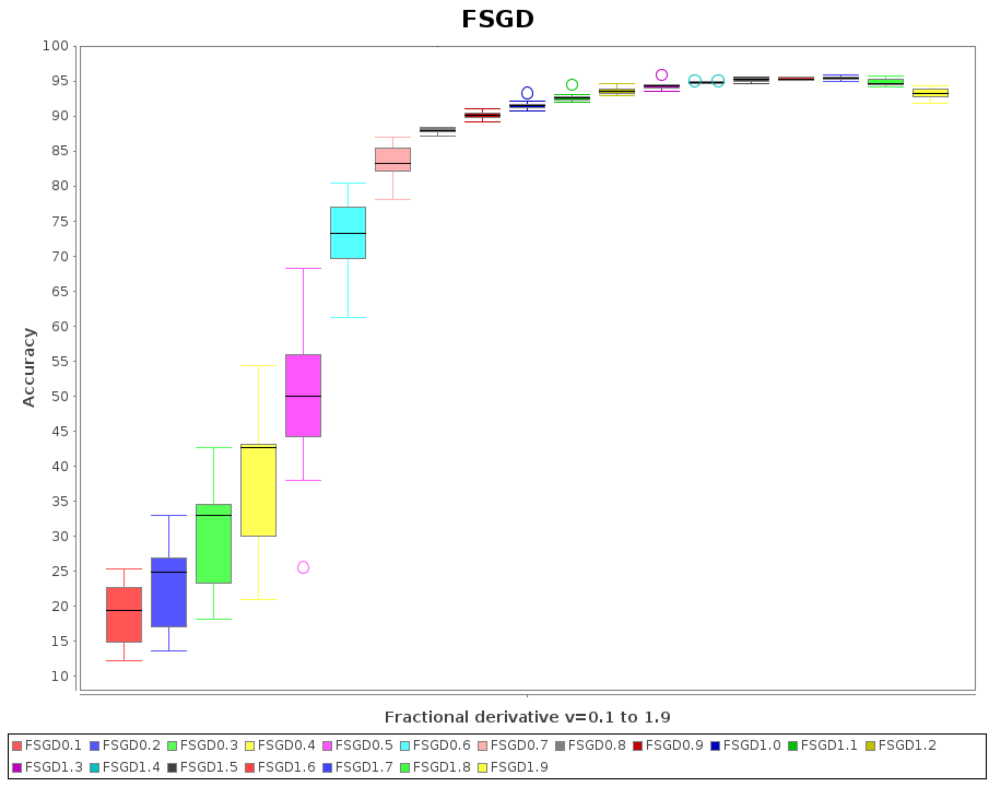
Figure 1, the boxplots of all data of
Table 2 are shown. In both of them, it is possible to appreciate the optimal performance for
(the average accuracy is
and the standard deviation is
). The improvement is about
better than SGD (
), and these values are highlighted in bold in
Table 2 for comparison purposes.
From the results of Experiment 1, the importance of the fractional gradient factor stands out, since the best performance is achieved for , instead of the traditional . It is shown that provides additional freedom degree to optimize the neural network parameters.
3.1.2. Experiment 1.2
This experiment considers FSGD with the same values for learning rate and momentum . The learning rate is increased 100 times with respect to Experiment , and then that aims to have a balance on their contribution to the weight updates. The fractional order varies from to with step = , and additionally , which corresponds to SGD as a special case.
The results of Experiment
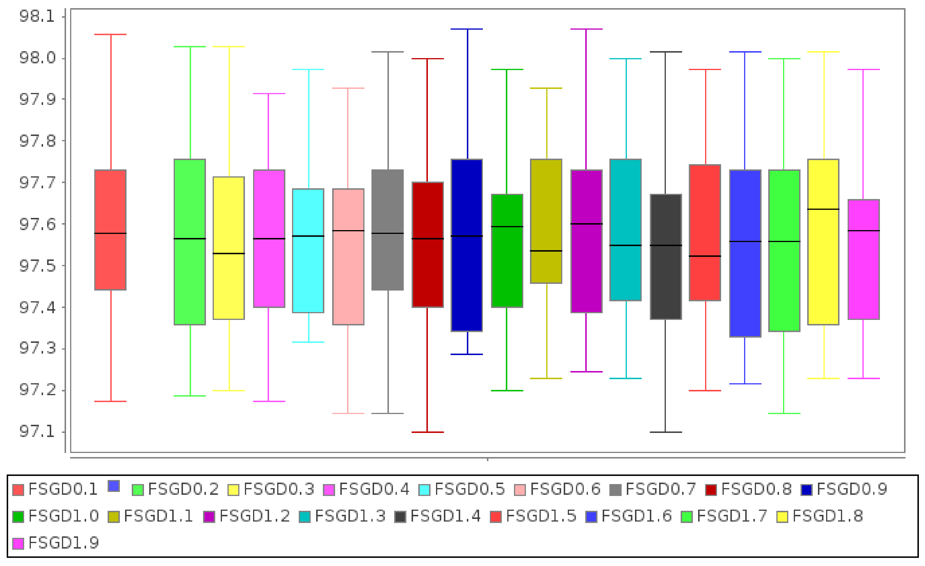
are shown in
Table 3 and
Figure 2, where it is possible to see (highlighted in bold in
Table 3) that cases
and
have better performance than others, including the case
which corresponds to SGD with momentum
. Although these cases in the last fold (see the last row of columns
and
) have a slightly smaller value than those of
, the rest of the data show a consistent enhancement over the rest of the folds, as it is illustrated in the boxplots of
Figure 2, where the boxplots for
and
are better positioned above the case
.
From Experiment , it is deduced that the use of momentum contributes to better performance close to , while FSGD without momentum in Experiment barely reaches about for the last fold.
3.1.3. Experiment 1.3
Other experiment considers FSGD with
and a high value for momentum
. The results are shown in
Table 4 together with the boxplots of
Figure 3. Additionally, in
Table 5, the correlation of the columns of
Table 4 are shown, and it is notorious the high correlation between all columns for different values of
to
, which means that a high value of momentum and low learning rate diminishes the effect of the fractional factor
. In fact, the correlation matrix of
Table 5 makes this evident since all the correlation values are higher than
, in spite of the value of
. Moreover, the performance for
decreases about
with respect to Experiment
with lower momentum
, as is appreciated when comparing
Table 3 and
Table 4.
3.2. Experiment 2
Experiment 2 uses the HAR dataset Actitracker [
29]. It was released by Wireless Sensor Data Mining (WISDM) lab and refers to 36 users using a smartphone in their pocket at a sample rate of 20 samples per second. The dataset contains acceleration values for
x,
y and
z axes, while the user performs six different activities in a controlled environment: downstairs, jogging, sitting, standing, upstairs, and walking. The number of samples is 1,098,209, which was originally split into
for training and
for testing.
To obtain better experimental support, these data were merged, and cross-validation with folds was applied with shuffle.
The source code was adapted from [
31], and it considers a 2D-convolutional neural network (2D-CNN) with two dense layers and ReLu activation function, followed by a softmax layer.
Fractional optimizers were studied in two groups based on their performance; the first group is FSGD, FSGDP, FAdagrad and FAdadelta, and the second group is FRMSProp, FAdam and FAdamP. It gives place to Experiments and .
3.2.1. Experiment 2.1
The source code of [
31] was modified to include FSGD, FSGDP, FAdagrad and FAdadelta.
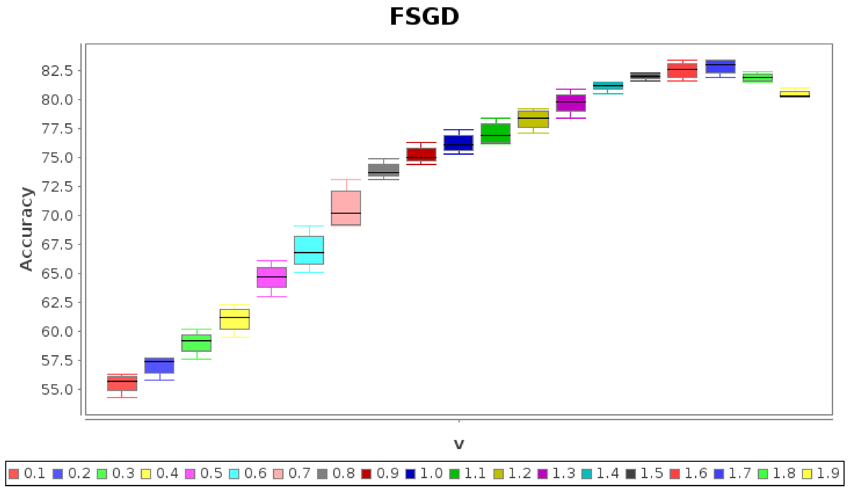
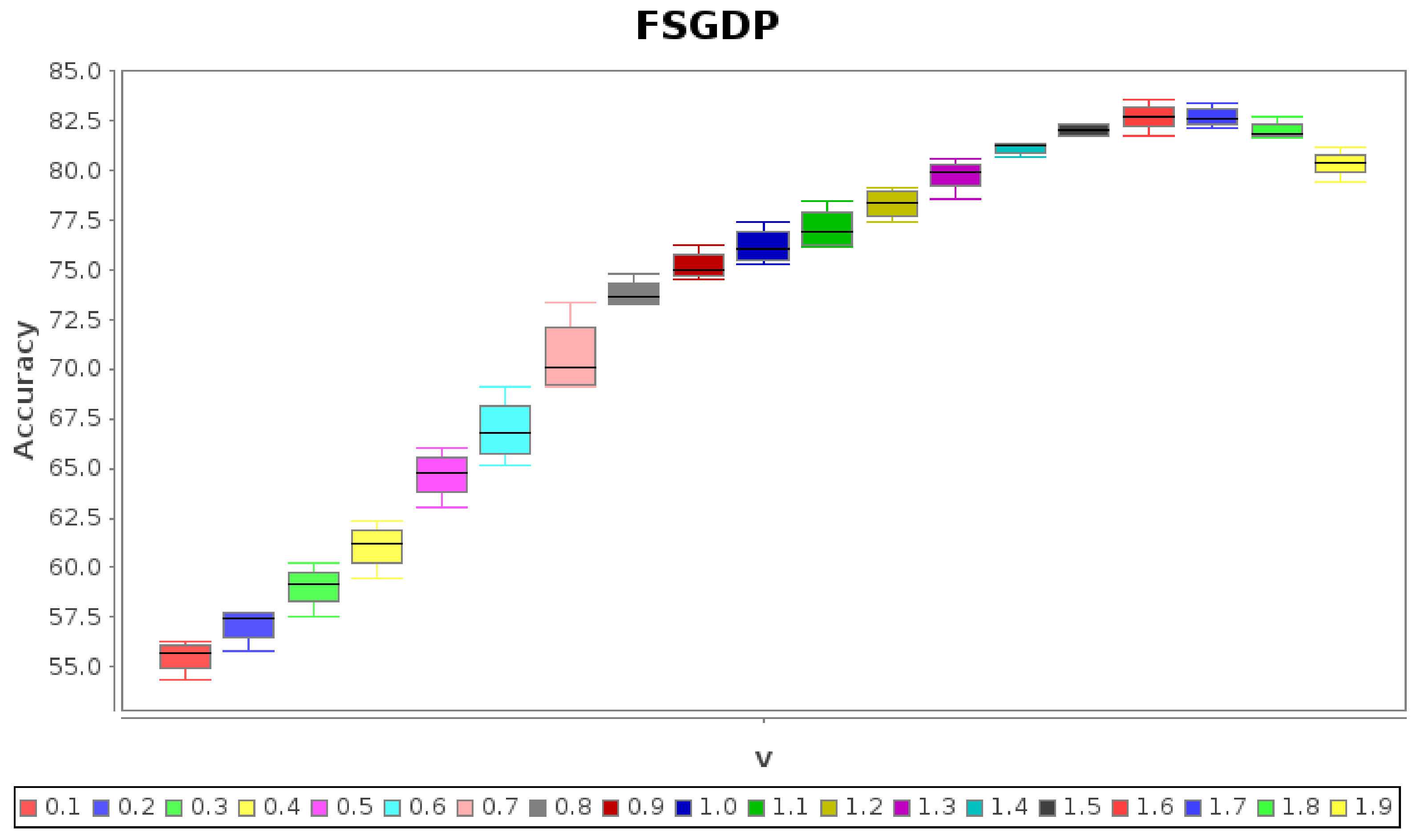
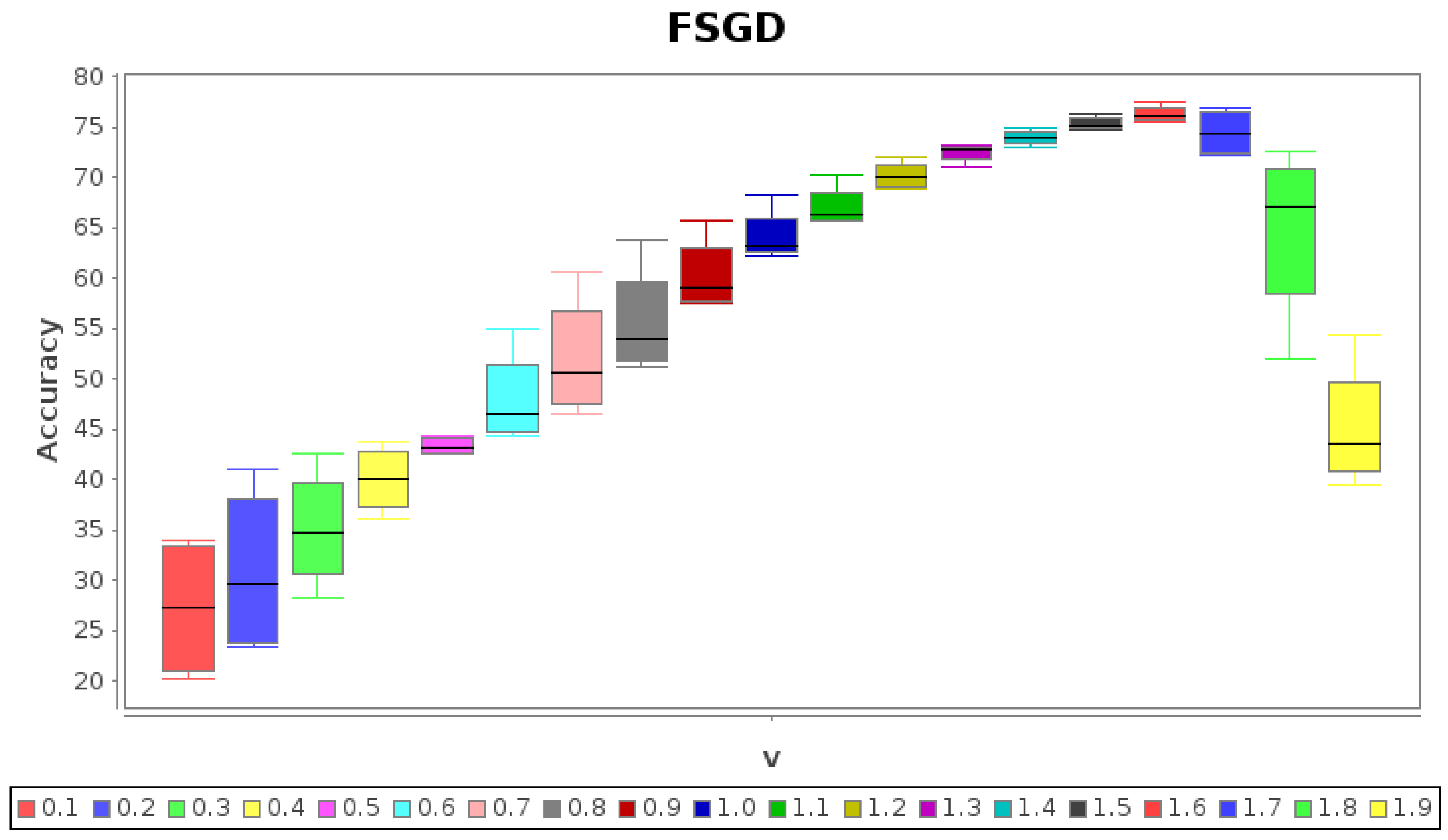
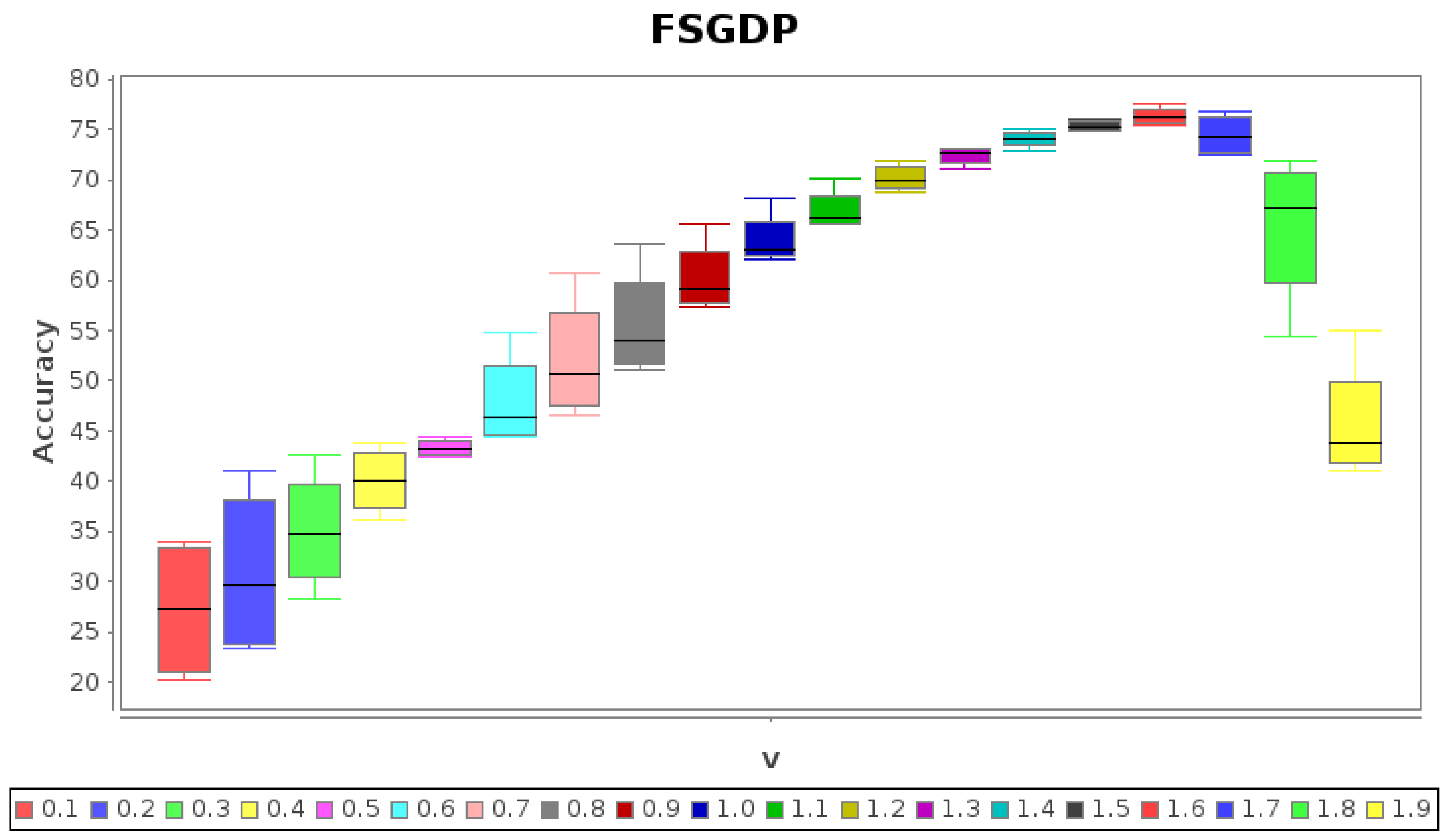
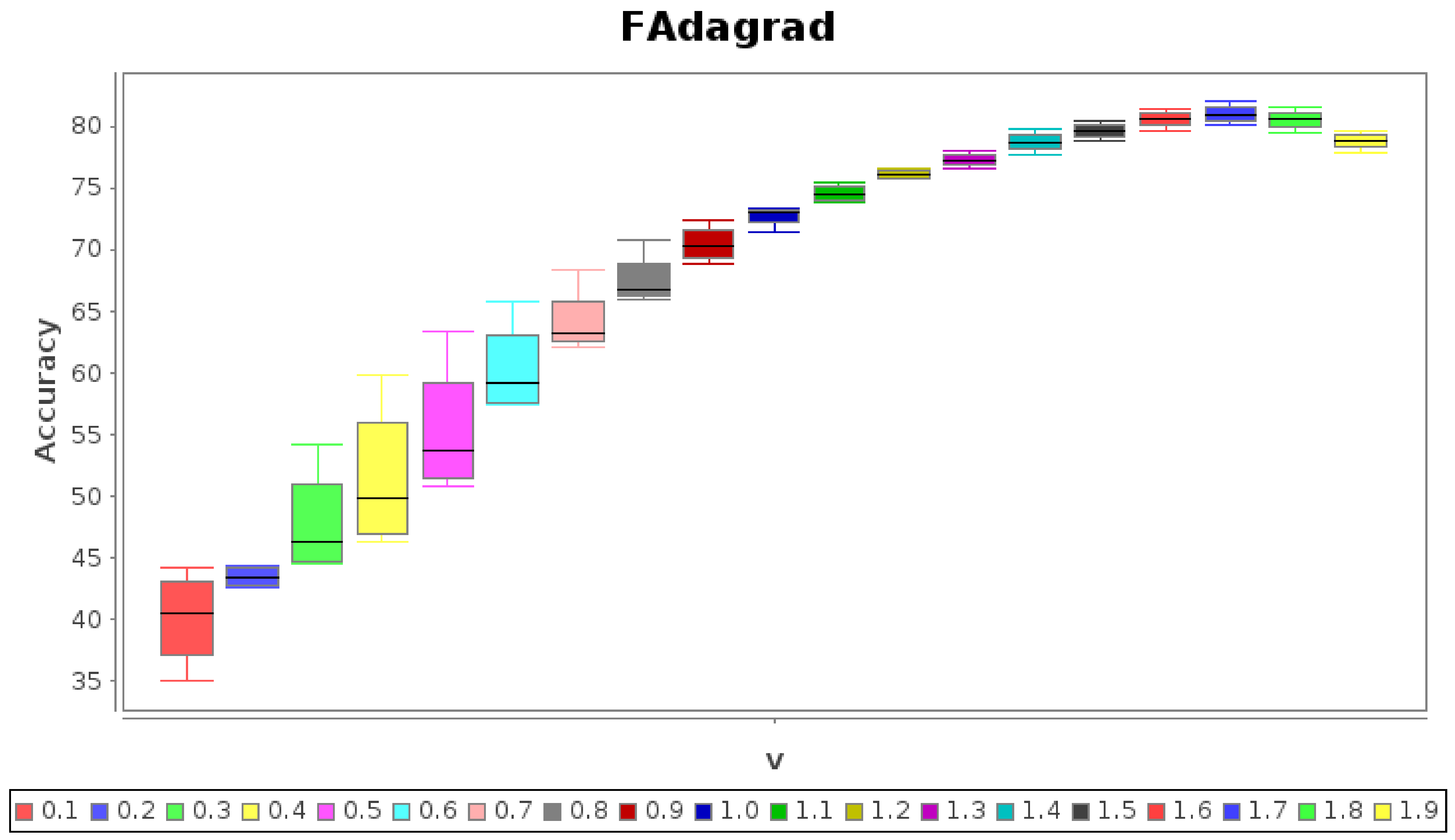
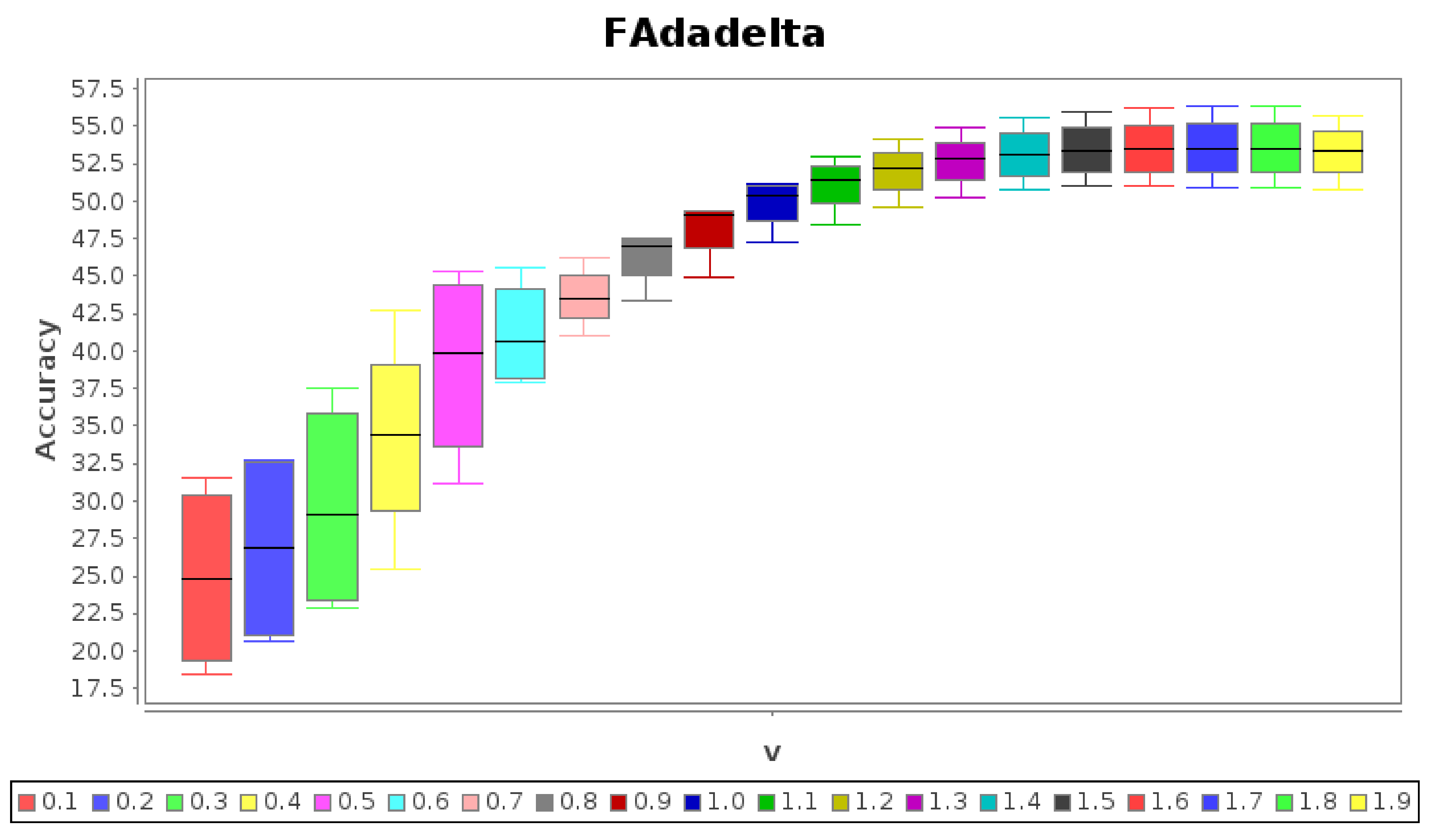
Because of space saving, the boxplots of accuracies for
folds are illustrated in
Figure 4,
Figure 5,
Figure 6 and
Figure 7, but tables with numerical data are not included. The following observations can be made:
Figure 4. The highest score for FSGD is
at
.
Figure 5. The highest score for FSGDP is
at
(a marginal difference with respect to FSGD).
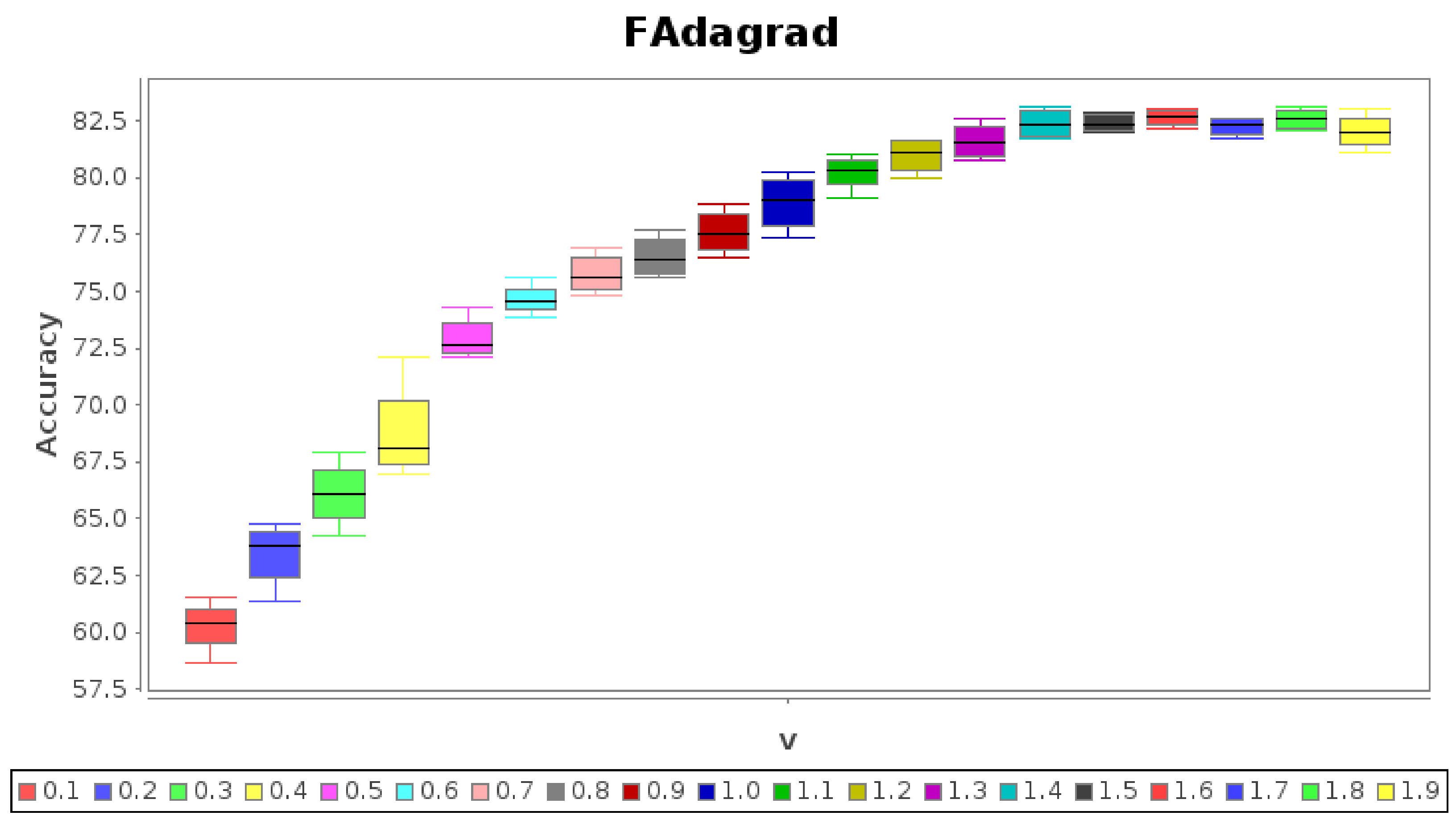
Figure 6. FAdagrad just reaches its maximum
at
.
Figure 7. The worst performance of these four optimizers is for FAdadelta with a maximum of
at
.
In this experiment, is obvious the influence of the fractional factor to enhance the performance compared with the traditional first-order case. However, these results are not the best possible because they can be improved by other optimizers, as will be shown in the next experiment.
3.2.2. Experiment 2.2
In Experiment 2.2, the modification to the source code of [
31] was to include fractional FRMSProp, FAdam and FadamP versions.
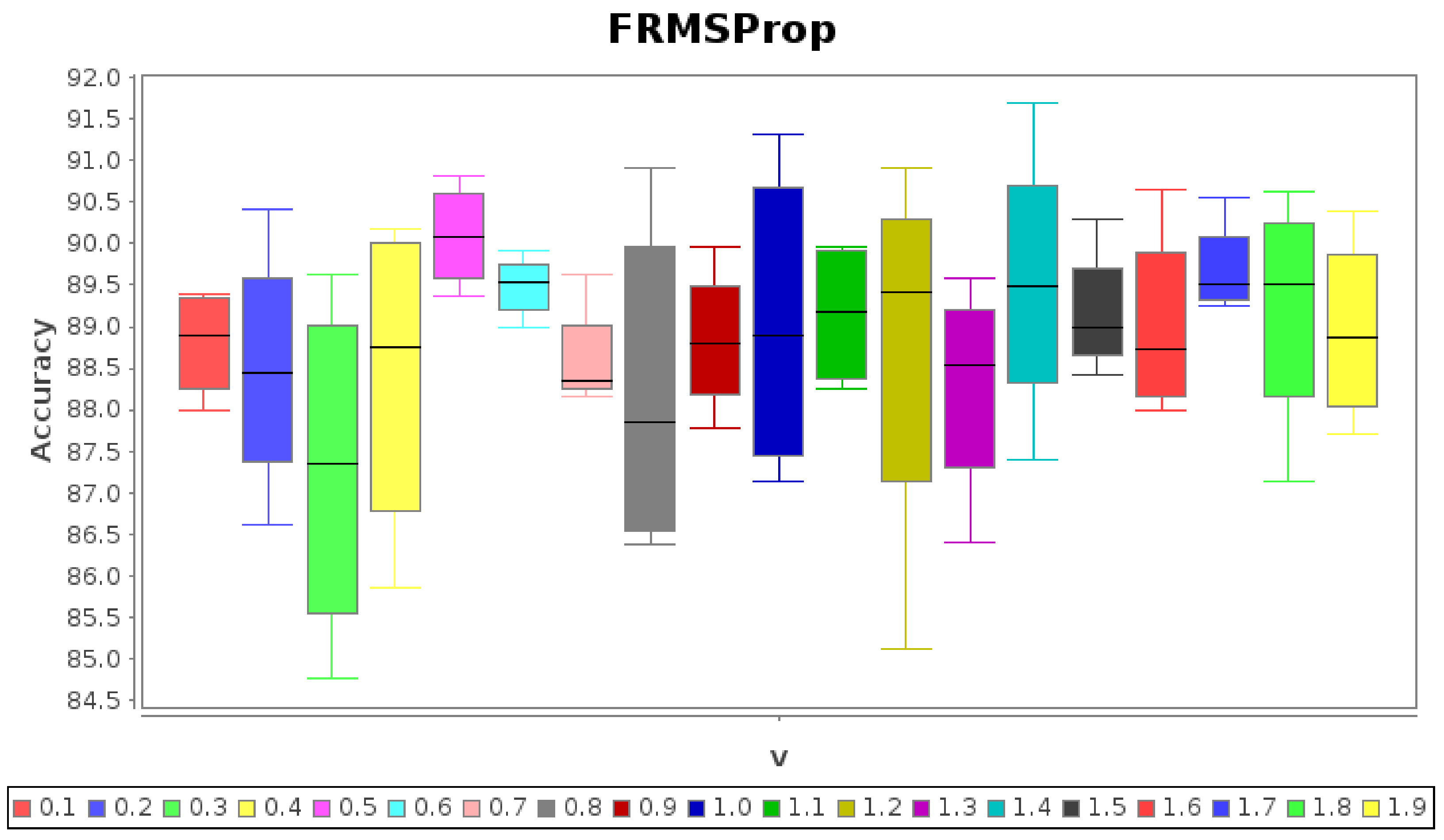
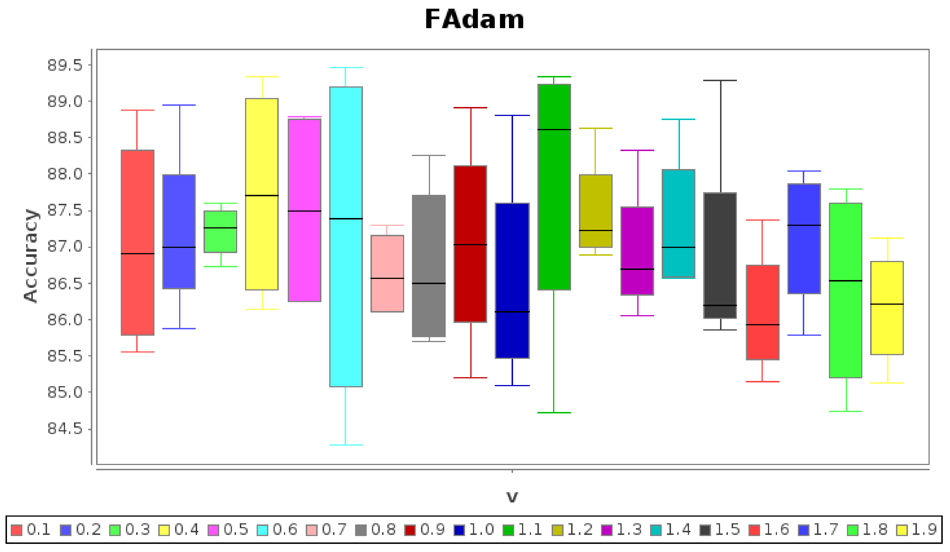
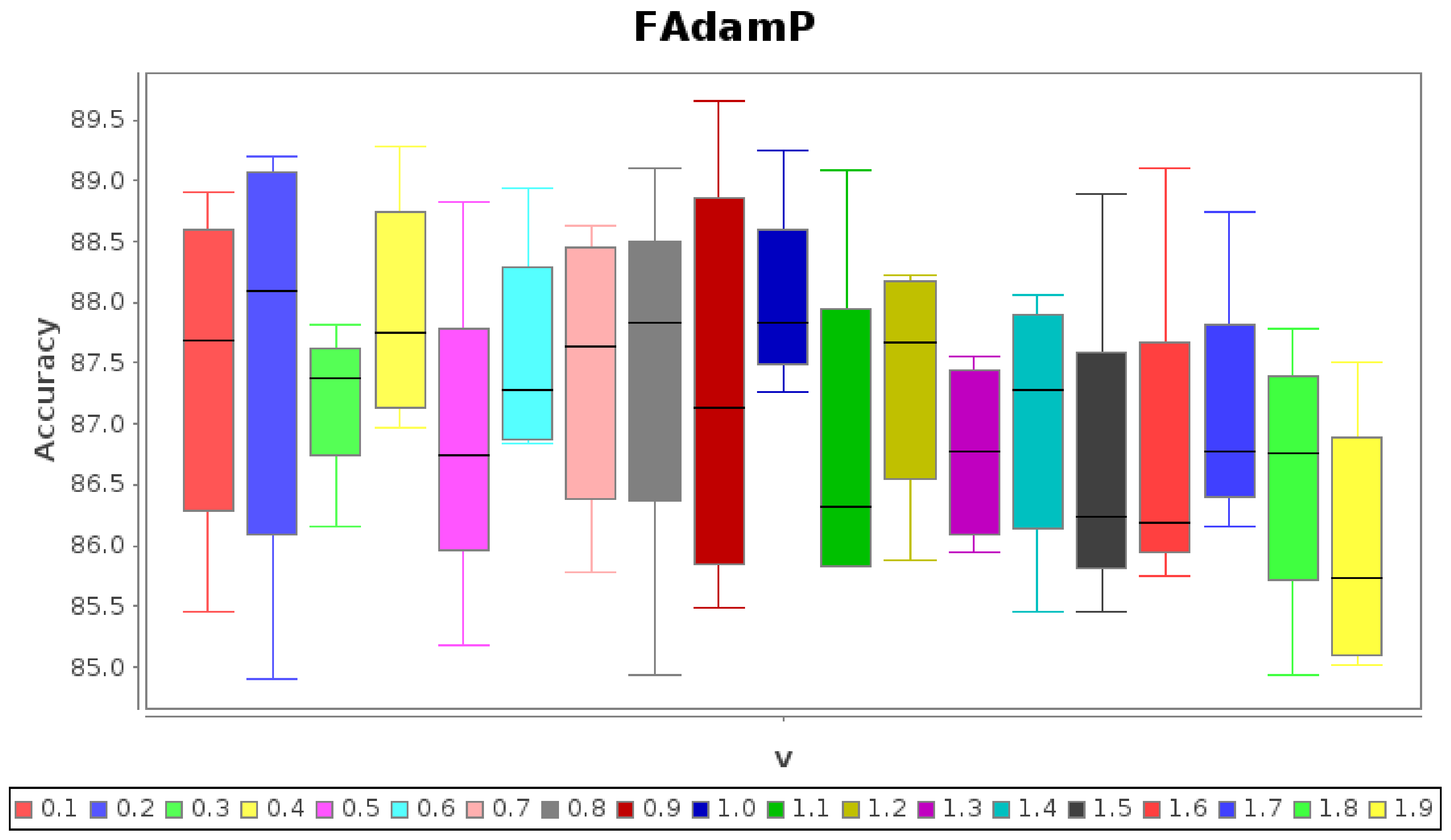
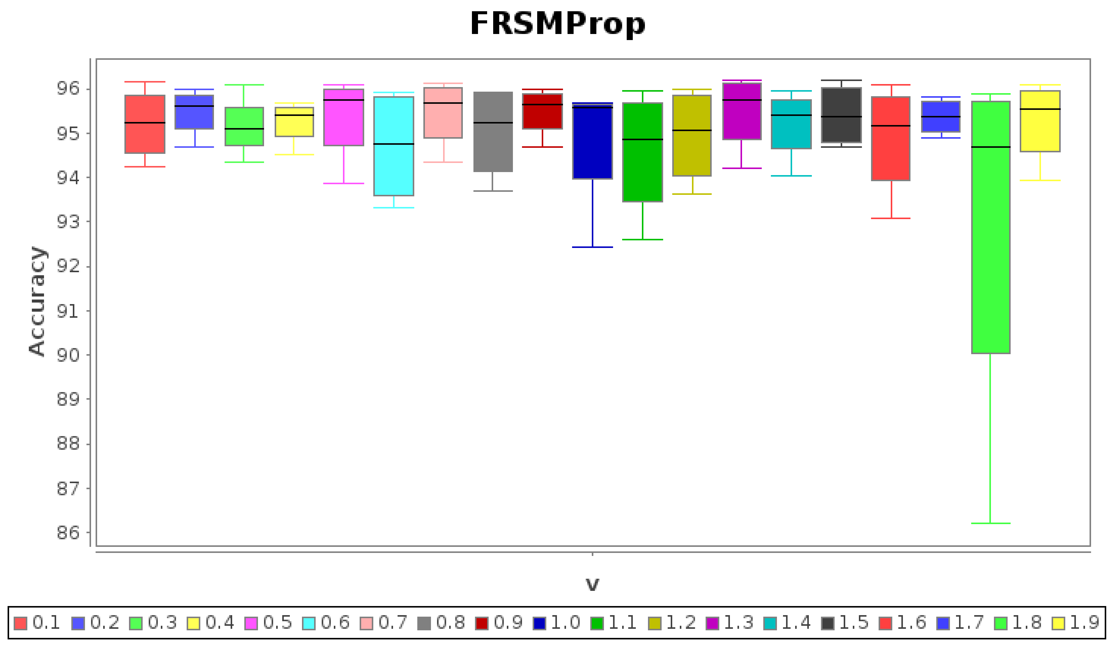
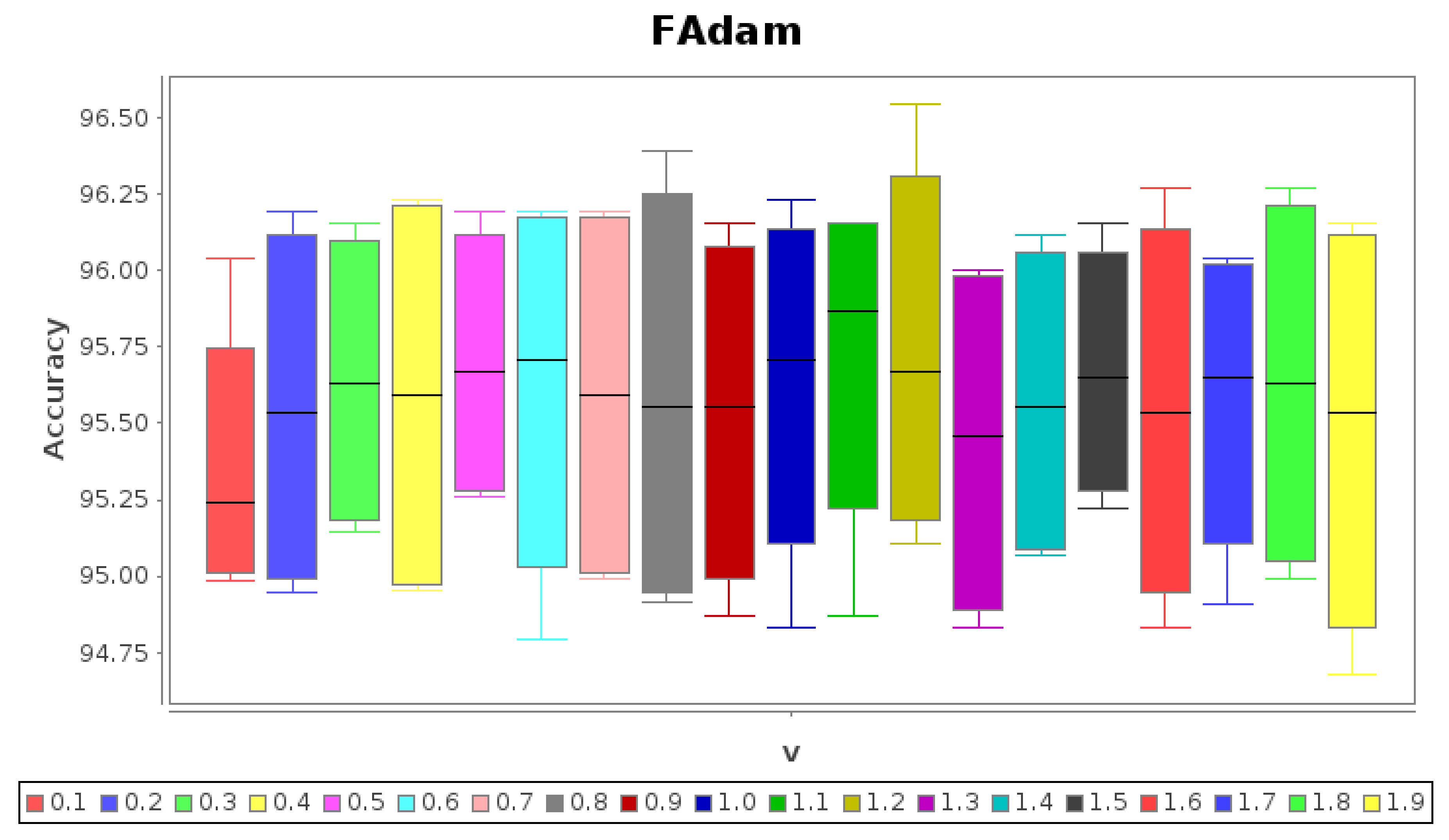
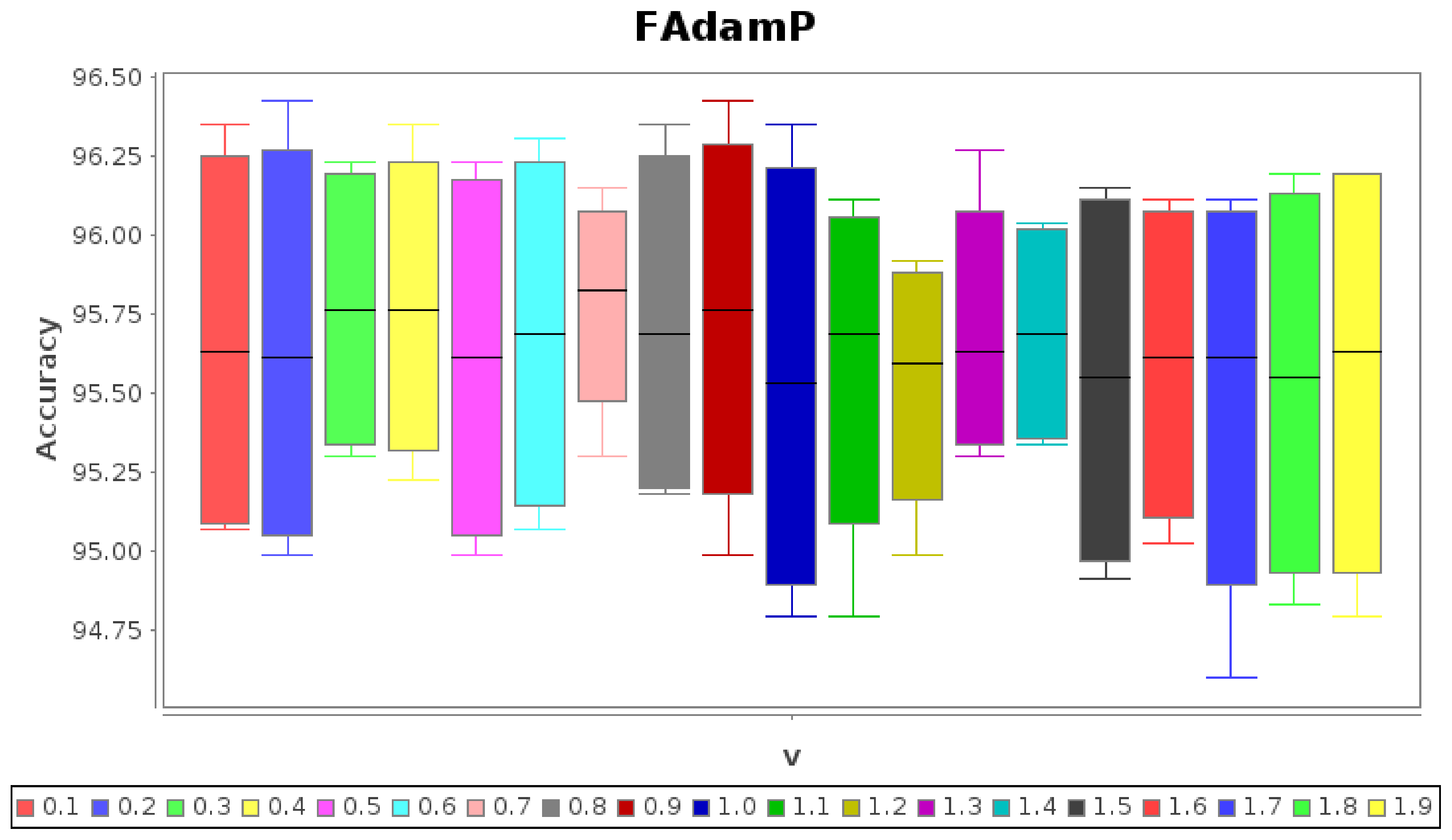
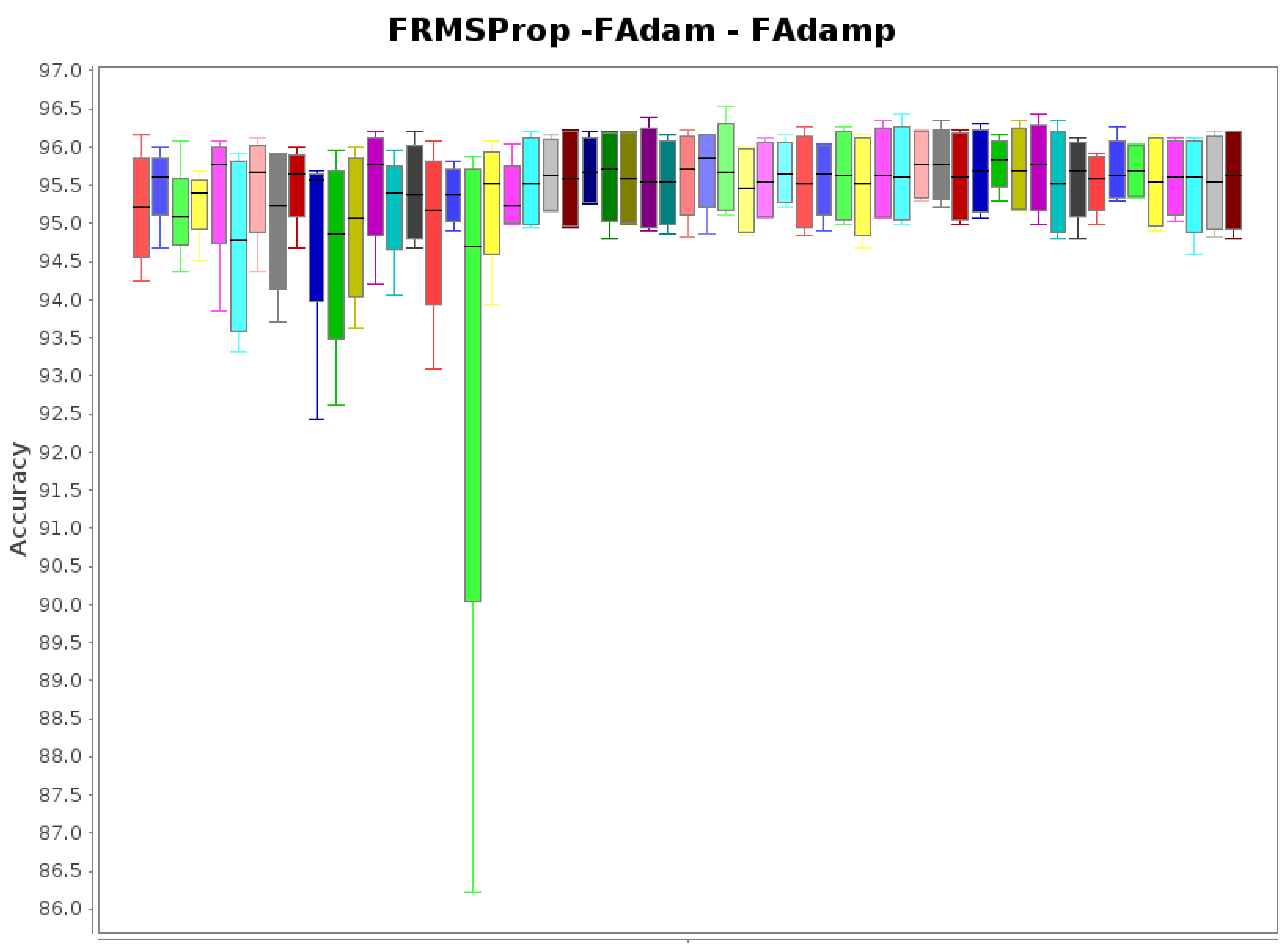
Figure 8,
Figure 9 and
Figure 10 show the boxplots from accuracies of the
folds for FRMSProp, FAdam and FadamP, respectively, with
in the interval
to
and step equals to
.
In
Figure 8, a few candidates can be identified as “the winners”, although there is no a strong dominant case. The most relevant cases of
Figure 8 are
FRSMProp at . This case has a superior and more compact behavior compared with the integer case .
FRSMProp at . This case has similar performance to that of RMSProp (, average and standard deviation ), but the case is slightly higher (average and standard deviation ).
In
Figure 9, FAdam with
can be considered better than for
since the first has an average accuracy equals to
(
over the case
) although it certainly has a slightly larger standard deviation (+0.43) than for the case
.
According to
Figure 10, FAdamP with
(i.e., AdamP) can be considered the best (just in FadamP category) since is not possible to identify a convincingly better case than accuracy
and standard deviation =
. However, when comparing group 2, FadamP is improved by FRSMProp at
.
In general, for this Experiment 2.2, the best cases correspond to FRSMProp, but it is also important to mention that group 2 outperformed the group 1 accuracies of Experiment .
3.3. Experiment 3
In Experiment 3, the dataset “Human Activity Recognition Using Smartphones” [
30] was used. It contains data from 30 subjects performing one of six activities: walking, walking upstairs, walking downstairs, sitting, standing and laying. The data were collected while wearing a waist-mounted smartphone, and the movement labels were manually obtained from videos.
Originally, the dataset was split into for training and for testing. Both training and testing subsets were mixed to obtain a unified dataset and to apply cross-validation with folds and shuffle, that produces a fold size of of the whole, which yields to for training and for testing, trying to match the original split of + .
The optimizers were studied with the same groups of Experiment 2, because of their behavior.
3.3.1. Experiment 3.1
The source code was adapted from [
32] to include optimizers FSGD, FSGDP, FAdagrad and FAdadelta. Crossfolding was applied for each optimizer, moving
from
to
with steps of
.
The learning rate was
and the momentum
was equal to
. The results for FSGD, FSGDP, FAdagrad and FAdadelta are shown in
Figure 11,
Figure 12,
Figure 13 and
Figure 14 as boxplots, where it is possible to see essentially the same tendency for each optimizer: increasing conform
increases to reach a maximum and then decreases. FSGD and FSGDP decrease abruptly for
(see
Figure 11 and
Figure 12). The highest average accuracies are at
for FSGD and FSGDP with accuracies of
and
, respectively.
In the case of
Figure 13 for FAdagrad, the maximum average accuracy is
at
. FAdadelta in
Figure 14 presents the worst performance, given that the maximum is
at
.
Again, in this experiment, it is possible to appreciate the influence of the fractional factor to modify the accuracy.
3.3.2. Experiment 3.2
In
Figure 15,
Figure 16 and
Figure 17, boxplots are shown for the accuracies of
folds of FRMSProp, FAdam and FadamP respectively.
From these three figures, the next relevant cases were observed for each case independently:
FRMSProp. In
Figure 15, the case
is improved by the rest of the cases, except
.
Fadam. In
Figure 16, the case
is improved by the accuracy at
.
FadamP. In
Figure 17, the case
is improved by the accuracy at
.
In this experiment, FRMSProp does not have better performance than FAdam and FAdamP; however, the fractional order seems to slightly modify the performance, and in most cases, a value other than provides better accuracy.
3.3.3. Experiment 3.3
Finally, the same experiments
and
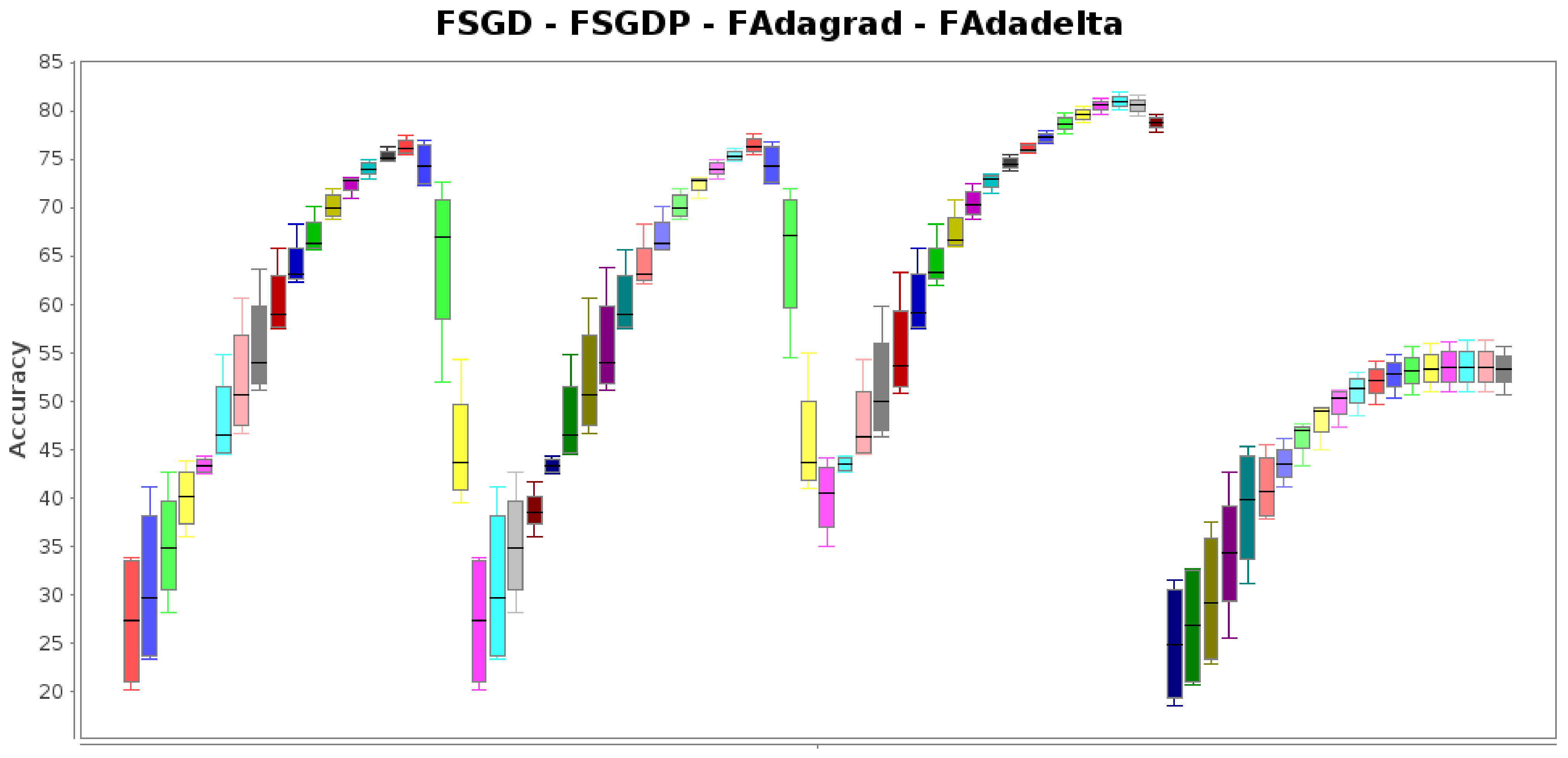
were repeated with 10 folds, and similar results were obtained. An overview of the accuracies of both groups, group 1 (FSGD, FSGDP, FAdagrad, FAdadelta) and group 2 (FRMSProp, Fadam, FAdamP), is shown as boxplots in
Figure 18 and
Figure 19. The boxplots correspond to each optimizer listed in groups 1 and 2, for
with increments of
.
In
Figure 18, it is possible to appreciate the highest accuracy for FAdagrad at
, whereas in
Figure 19, the highest accuracy is for FAdam at
.
Once the experiments have been carried out, it is convenient to mention that, similar to the integer case, a geometric interpretation can be given to Equation (
24) as a gradient at the region of interest on the error surface. The main benefit of fractional
v-derivative over the integer version is the expansion of the region of search around the test point given by
v and the weights
[
33]. In this sense, the benefit is provided by the factor
of Equation (
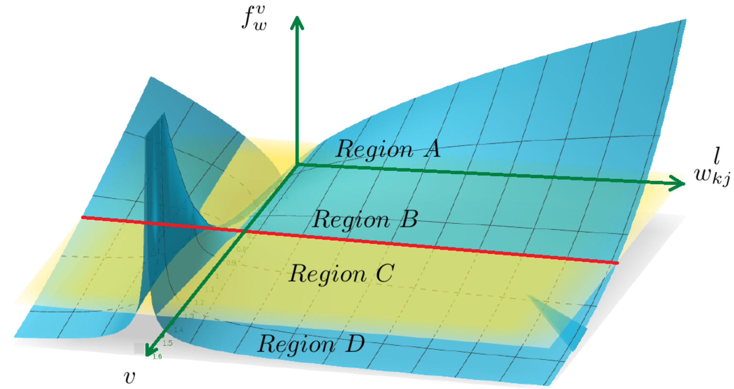
25), and to explore the effect of non-locality, a 3D plot is shown in
Figure 20. It is possible to identify four regions with different behavior:
Region A: For . The factor follows and it could produce divergence for and consequently for , and for the fractional gradient .
Region B: For . The integer case corresponds to the red line . No context information is considered, just the local point.
Region C: For . The surface reaches a local maximum at for .
Region D: For . tends to zero as fast as increases. It promotes that small weights increase its values and move to the flatter region, where they will stabilize.
The Cartesian axes in
Figure 20 are as follows:
x-axis. The weights .
y-axis. Fractional value .
z-axis. The fractional factor that modifies the integer order gradient.
In
Figure 20 there is a yellow plane at
used as reference for the red line of the integer case.
It is noteworthy that in region C, the experimental accuracies of the fractional optimizers (depending of v) follow a similar behavior to . For now, it is just an observation that merits exploring the possible relationship between the optimal fractional order and the region of best accuracy for fractional optimizers.
4. Discussion
Unlike other optimizers that have been proposed, alluding mainly to concepts such as momentum or velocity, in this paper, gradient descent variants are proposed based on fractional calculus concepts, and specifically on the Caputo fractional derivative.
The proposed fractional optimizers add the prefix “F” to original names, and their update formulas essentially aggregate the factor defined in such a way that the limit exists when the v-order derivative tends to 1, which leads to a more general formula that includes the integer order as a special case.
Fractional optimizers are slightly more expensive computationally because they require computing the factor. However, they are still very competitive because the computation is performed efficiently through Tensorflow, and the additional advantage is that the fractional factor transfers non-local exploring properties, rather than just considering an infinitely small neighborhood around a point on the error surface as in the integer case, which experimentally is traduced in the improvement of the performance of fractional optimizers.
The fractional factor provides an additional degree of freedom to the backpropagation algorithm, and consequently, to the learning capacity of neural networks, as was shown in several experiments.
The fractional optimizers were successfully implemented in Tensorflow–Keras with modifications to the original source code to obtain FSGD, FSGDP, FAdagrad, FAdadelta, FRMSProp, FAdam and FAdamP classes. Everything indicates that it is possible to apply the same methodology to modify other gradient-based optimizers, as well as making implementations in other frameworks.
Three experiments were carried out with MNIST and two HAR datasets. The results on crossfolding show that in all the experiments, a fractional order provides better performance than the first order for the same neural network architectures.
In the experiments, FSGD, FSGDP, FAdagrad and FAdadelta (group 1) basically follow the same pattern of increasing their performance as the -order does, obtaining a maximum and then decreasing.
Other optimizers, such as FRMSProp, FAdam and FAdamP (group 2), do not follow the same pattern, and seem to be less susceptible to the fractional order change. From the experiments, it can be said that FRMSProp has an “intermediate” pattern between the optimizers of group 1 and group 2.
Even so, essentially in all the experiments, the best performing derivative order was a fractional value.
Therefore, based on the results, it is possible to affirm that fractional derivative gradient optimizers can help to improve the performance on the training and validation task, and opens the possibility to include more fractional calculus concepts to neural networks applied to HAR.
The Tensorflow–Keras implementations of this work are available in a repository to contribute to the deep learning and HAR communities to improve and apply these techniques based on fractional calculus.
Future works include exploring more fractional derivative definitions and HAR datasets with fractional regularization factors as well as studying the effects in vanishing gradient problems with other neural network architectures.


