An Iterative Guidance and Navigation Algorithm for Orbit Rendezvous of Cooperating CubeSats

Abstract

Modern space missions often require satellites to perform guidance, navigation, and control tasks autonomously. Despite their limited resources, small satellites are also involved in this trend, as in-orbit rendezvous and docking maneuvers and formation flying have become common requirements in their operational scenarios. A critical aspect of these tasks is that these algorithms are very much intertwined with each other, although they are often designed completely independently of one another. This paper describes the design and simulation of a guidance and relative navigation architecture for the rendezvous of two cooperating CubeSats. The integration of the two algorithms provides robustness to the solution, by simulating realistic levels of noise and uncertainty in the guidance law implementation. The proposed guidance law is derived based on the linearized equations of orbital motion, written in terms of spherical coordinates. The trajectory is iteratively corrected at a fixed time step, so that errors from the navigation and the initial orbital condition can be recovered. The navigation algorithm processes the bearing and range measurements from a camera and an intersatellite link through an unscented filter to provide the information required from the guidance law. A Monte Carlo campaign based on a 3-DOF simulation demonstrates the effectiveness of the proposed solution.

1. Introduction

The use of small satellites in modern space missions has become an important factor in the aerospace industry, thanks to the versatility, reliability, and low cost of these platforms. As the scenarios involving small satellites are growing in numbers and complexity, more advanced technological solutions are needed to address the new tasks of these missions. Autonomous guidance, navigation, and control (GNC) systems for small satellites, for example, are crucial for implementing challenging tasks, such as rendezvous and docking [1], formation flying [2], and space debris removal [3].

Guidance algorithms for rendezvous are usually based on the classical Hill–Clohessy–Wiltshire (HCW) equations, either under the impulsive thrust approximation or assuming finite thrust. Seminal publications on impulsive rendezvous have been written by Prussing [4,5], who investigated minimum-fuel rendezvous trajectories including two, three, or four velocity changes. By using the HCW equations, Carter [6] focused on finite thrust rendezvous with an upper bound on thrust magnitude, and proved that at most seven thrust/coast intervals can occur. Later, Carter and Humi [7] investigated fuel-optimal rendezvous relative to a point in a general Keplerian orbit, and demonstrated that no singular arc exists if the orbit is noncircular. Most recently, Pontani and Conway [8] addressed the problem of finding a variety of minimum-fuel rendezvous trajectories by using finite thrust and proved a remarkable symmetry property of optimal rendezvous paths. Although all the preceding contributions employ the HCW equations, Prussing and Chiu used the nonlinear equations of Keplerian motion, for the purpose of minimizing fuel consumption [9] under the impulsive thrust approximation. Pontani et al. [10] found both impulsive and finite thrust, fuel-optimal rendezvous trajectories by using a particle swarm algorithm. Other works use alternative deterministic and heuristic methods for rendezvous optimization and guidance, such as the glideslope multipulse technique [11], optimally timed trajectory correction maneuvers [12], ${\mathcal{H}}_{\infty }$ and $\mu$-synthesis techniques [13]. However, in actual operational scenarios, rendezvous trajectories are affected by orbit perturbations, which make both the HCW linear equations and the Keplerian nonlinear equations relatively inaccurate for precise orbit rendezvous. Moreover, the assumption of perfect information on the relative spacecraft dynamics is not realistic, and an accurate rendezvous is likely to be infeasible without an effective navigation system, due to measurement noise or unavailable variables needed to compute the guidance command. This circumstance points out the need of an integrated, iterative guidance and navigation architecture, capable of performing correction maneuvers on the basis of the estimated state provided by the navigation system.

This paper analyzes the design of a relative guidance and navigation architecture for the rendezvous of two CubeSats, a target and a chaser, which are assumed to travel orbits in close proximity. The proposed guidance algorithm is based on the iterative application of the HCW linear equations of motion [14], written in terms of spherical coordinate displacements, under the assumption that both vehicles travel nearby orbits with small eccentricities. This simple approach aims at finding the correction maneuvers, modeled as impulsive velocity changes, that are necessary to maintain the chaser on track to the target. The orbital motion of both spacecraft is described by integrating the nonlinear equations of motion, which can include all the orbit perturbations relevant to the dynamical context.

The iterative nature of the guidance strategy allows accounting for the update of the target estimated orbit, provided by the navigation state, which is obtained from the measurements of the on-board sensors. Small space platforms have light architectures and weight constraints that require innovative navigation solutions, such as vision-based navigation. With this approach, a single [15] camera or multiple [16] cameras are employed on the chaser to measure the angular displacement to the target. A problem arising with the single-camera solution is the unavailability of relative range information [17], which affects the accuracy of the guidance law unless specific maneuvers are realized to improve the range observability [18,19]. Range becomes observable if the camera is offset with respect to the center of mass of the chaser [20], but not if the camera is placed in the line of sight between the target and the chaser, which is often the case. A thorough analysis of the performance of monocular visual navigation system is presented in [21]. Another possibility arises when the target is cooperative: in this case, direct range measurement becomes available thanks to an on-board intersatellite link (ISL), as in the case of the Milani 6U CubeSat mission [22].

The relative navigation solution is provided in real time by a recursive state estimator of the Kalman filter family of algorithms. Given the nature of the relative navigation equations, nonlinear Kalman filters are needed for this task, such as the extended Kalman filter (EKF) and the unscented filter (UF). The EKF has been a standard in relative navigation problems for a long time [23,24]. However, EKF’s poor performance against highly-nonlinear systems and even divergences have led to the wide adoption of the UF, for navigation problems in either its regular [25] or square-root [26] versions. In fact, the UF provides a more accurate and robust solution to the estimation problem [27] than EKF; therefore UF is chosen for this work.

The paper is organized as follows: the mathematical model that represents the relative motion of the spacecraft is described in Section 2; the design of the guidance and navigation algorithms is given in Section 3; the setup of the numerical simulations and the results are presented in Section 4; conclusions and final remarks are given in Section 5.

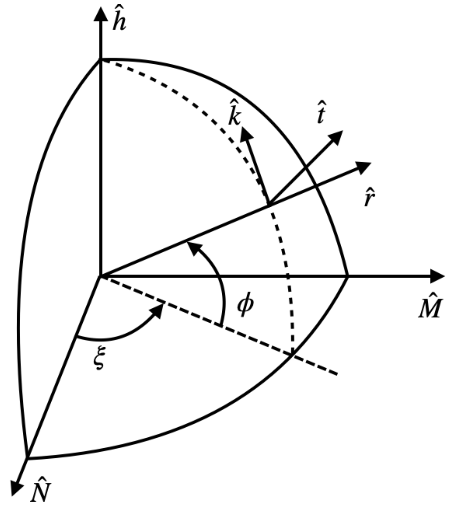
2. Equations of Motion

In order to write the equations of the relative orbital motion, a reference Keplerian circular orbit is defined in an inertial reference frame with axes $\widehat{N}$, $\widehat{M}$, $\widehat{h}$, as seen in Figure 1. Axes $\widehat{N}$ and $\widehat{h}$ are aligned respectively with the line of the ascending node and the angular momentum of the reference Keplerian orbit. The latter is circular and therefore has a fixed radius $R_R$, inclination $i_R$, and RAAN ${\mathsf{\Omega }}_R$. In the preceding frame, orbital motion of a space vehicle (subject to thrust and perturbing accelerations) is identified by the instantaneous radius r, right ascension $\xi$, declination $\varphi$, radial velocity $v_r$, transverse velocity $v_t$, and normal velocity $v_k$. Using these variables the equations of orbital motion are:

$$\begin{array}{cc}\left\{\begin{array}{c}\dot{r}=v_r\hfill \\ \dot{\xi }={\displaystyle \frac{v_t}{rcos\varphi }}\hfill \\ \dot{\varphi }={\displaystyle \frac{v_k}{r}}\hfill \end{array}\right.& \left\{\begin{array}{c}{\dot{v}}_r=-{\displaystyle \frac{\mu }{r^2}}+{\displaystyle \frac{v_t^2+v_k^2}{r}}+a_r\hfill \\ {\dot{v}}_t={\displaystyle \frac{v_t}{r}}(v_{k}tan\varphi -v_r)+a_t\hfill \\ {\dot{v}}_k=-{\displaystyle \frac{v_t^2}{r}}tan\varphi -{\displaystyle \frac{v_r{v}_k}{r}}+a_k\hfill \end{array}\right.\end{array},$$

(1)

where $\mu$ is the gravitational parameter of the main attracting body and $\overrightarrow{a}=\{a_r,a_t,a_k\}$ is the vector containing the three components of the external accelerations, due to either thrust or orbital perturbations.

The guidance law is obtained by linearizing Equation (1) around the reference orbit, assuming that the variables are perturbed by small displacements, denoted with $\delta$, from the respective values, associated with the reference circular orbit, i.e.,

$$\begin{array}{cc}\left\{\begin{array}{c}r=R_r+\delta r\hfill \\ \xi ={\xi }_r+\delta \xi \hfill \\ \varphi ={\varphi }_r+\delta \varphi \hfill \end{array}\right.& \left\{\begin{array}{c}{v}_r=v_{rR}+\delta v_r=\delta v_r\hfill \\ v_t=v_{tR}+\delta v_t=\sqrt{{\displaystyle \frac{\mu }{R_r}}}+\delta v_t\hfill \\ v_k=v_{kR}+\delta v_k=\delta v_k\hfill \end{array}\right.\end{array},$$

(2)

At this point, it is useful to define a new set of coordinates:

$$x=\delta r,y=R_R\delta \xi ,z=R_R\delta \varphi .$$

(3)

By using the definitions in Equations (2) and (3), expanding Equations (1) to the first order, and neglecting higher-order terms, the well-known Hill–Clohessy–Wiltshire (HCW) equations are obtained, in terms of spherical coordinates x, y, z,

$$\left\{\begin{array}{c}\ddot{x}-3{\omega }_R^{2}x-2{\omega }_R\dot{y}=a_r\hfill \\ \ddot{y}+2{\omega }_R\dot{x}=a_t\hfill \\ \ddot{z}+{\omega }_R^{2}z=a_k\hfill \end{array}.\right.$$

(4)

3. Guidance and Navigation

This section describes the guidance and navigation scheme used for the rendezvous of the two satellites. The guidance law is an iterative algorithm that calculates the steering maneuvers to achieve the final position of the target, using the available information on the position and velocity of both vehicles. The navigation subsystem estimates the information needed to calculate the guidance command by using the measurements from the on-board sensors. In this paper, it is assumed that an ISL and a camera provide range and bearing measurements.

3.1. Guidance

This work assumes that both the chaser and the target travel orbits sufficiently close to the reference circular Keplerian orbit. This implies that the orbital dynamics of both vehicles can be described by using the HCW Equation (4). Let $\delta \mathbf{r}:=\left[xyz\right]$ and $\delta \mathbf{v}:=\left[\dot{x}\dot{y}\dot{z}\right]$. Due to the linear nature of the governing Equation (4), the time evolution of the displaced position and velocity vectors $\delta \mathbf{r}\left(t\right)$ and $\delta \mathbf{v}\left(t\right)$ is given by [14]

$$\left[\begin{array}{c}\delta \mathbf{r}\left(t\right)\hfill \\ \delta \mathbf{v}\left(t\right)\hfill \end{array}\right]=\left[\begin{array}{cc}M\left(\tau \right)& N\left(\tau \right)\\ S\left(\tau \right)& T\left(\tau \right)\end{array}\right]\left[\begin{array}{c}\delta \mathbf{r}\left(t_k\right)\hfill \\ \delta \mathbf{v}\left(t_k\right)\hfill \end{array}\right],$$

(5)

where $\tau =t-t_k$. The closed-form expressions of the $(3\times 3)$ matrices M, N, S, and T are reported in [14].

The rendezvous maneuver is assumed to have a specified duration $\Delta t_{tot}$. At a generic time $t_k$ ($0\le t_k\le \Delta t_{tot}$), the maneuver at hand can be designed by using Equation (4), by including a pair of impulsive changes of velocity, the first at time $t_k$ and the second at time $\Delta t_{tot}$. Superscripts + and − are associated with the time instants immediately before and after each velocity changes, i.e.,

$$\left\{\begin{array}{c}\Delta {\mathbf{v}}_1=\delta \mathbf{v}\left(t_k^{+}\right)-\delta \mathbf{v}\left(t_k^{-}\right)\hfill \\ \Delta {\mathbf{v}}_2=\delta \mathbf{v}(\Delta t_{tot}^{+})-\delta \mathbf{v}(\Delta t_{tot}^{-})\hfill \end{array}\right..$$

(6)

The final goal is to get the position and velocity of the target at time $\Delta t_{tot}$, i.e.,

$$\left\{\begin{array}{c}\delta \mathbf{r}(\Delta t_{tot})=\Delta {\mathbf{r}}_T\left(t_{tot}\right)\hfill \\ \delta \mathbf{v}(\Delta t_{tot}^{+})=\Delta {\mathbf{v}}_T\left(t_{tot}\right)\hfill \end{array}\right.,$$

(7)

where subscript T refers to the target. The magnitudes and directions of $\Delta {\mathbf{v}}_1$ and $\Delta {\mathbf{v}}_2$ are given by the following vector equations, obtained by combining the previous relations

$$\left\{\begin{array}{c}\Delta {\mathbf{v}}_1=N_f^{-1}\left[\delta {\mathbf{r}}_T(\Delta t_{tot})-\Delta \mathbf{r}\left(t_k\right)\right]-\delta \mathbf{v}\left(t_k^{-}\right)\hfill \\ \Delta {\mathbf{v}}_2=\delta {\mathbf{v}}_T(\Delta t_{tot})-\left[S_f\delta \mathbf{r}\left(t_k\right)+T_f\delta \mathbf{v}\left(t_k^{+}\right)\right]\hfill \end{array}\right.,$$

(8)

where subscript f denotes the value of the respective matrix, evaluated at $\tau =\Delta t_{tot}-t_k$. Let $\Delta t_S$ represent the time interval between two consecutive iterations. The guidance algorithm is based on the following iterative steps, to perform at each time $t_k$:

• calculate $t_{k+1}=t_k+\Delta t_S$; if $t_{k+1}\ge \Delta t_{tot}$, then set $t_{k+1}=\Delta t_{tot}$;
• evaluate the displacement vectors $\delta \mathbf{r}$ and $\delta {\mathbf{v}}_1$ at $t_k^{-}$;
• calculate $\Delta {\mathbf{v}}_1$ by using Equation (8);
• using the definitions of the displaced position and velocity coordinates, obtain the spherical coordinates of position and velocity of the chaser (r, $\xi$, $\varphi$, $v_r$, $v_t$, $v_k$) at $t_k$;
• propagate numerically the nonlinear Equation (1) in the interval $[t_k,t_{k+1}]$;
• if $t_{k+1}=\Delta t_{tot}$, then evaluate $\delta {\mathbf{v}}_2$ at $\Delta t_{tot}$.

It is worth remarking that the algorithm at hand evaluates iteratively $\delta {\mathbf{v}}_1$, whereas $\delta {\mathbf{v}}_2$ is evaluated only at the final time.

3.2. Navigation

The navigation system consists of an algorithm that processes the available measurements $\zeta$ to reconstruct the target estimated state $\widehat{\chi }$, defined as

$$\widehat{\chi }=\{{\widehat{r}}_T,{\widehat{\xi }}_T,{\widehat{\varphi }}_T,{\widehat{v}}_{r_T},{\widehat{v}}_{t_T},{\widehat{v}}_{k_T}\}.$$

(9)

The model assumed for the motion of the target is that of Equation (1), where the external accelerations $\overrightarrow{a}$ are considered to be null, i.e., the target is not maneuvering and no orbital perturbations are considered. The equations that describe the three measurements (one distance, and two angles) are the following:

$$\left\{\begin{array}{c}{\zeta }_1=\left|\right|(x_2-x_1,y_2-y_1,z_2-z_1)\left|\right|+{\nu }_{range}\hfill \\ {\zeta }_2=arctan{\displaystyle \frac{y_2-y_1}{x_2-x_1}}+{\nu }_{bear1}\hfill \\ {\zeta }_3=arctan{\displaystyle \frac{z_2-z_1}{\sqrt{{(x_2-x_1)}^2+{(y_2-y_1)}^2}}}+{\nu }_{bear2}\hfill \end{array}\right.,$$

(10)

where ${\nu }_{range}\in \mathcal{N}(0,{\sigma }_{{\nu }_{range}})$, ${\nu }_{bear1}\in \mathcal{N}(0,{\sigma }_{{\nu }_{bear}})$ and ${\nu }_{bear2}\in \mathcal{N}(0,{\sigma }_{{\nu }_{bear}})$ are three random signals representing the noise on the measurements, whereas subscripts 1 and 2 correspond to the two satellites. Because of the optical nature of the sensor, the intensity of the noise signal on the range measurement depends on the distance between the two spacecraft. Therefore, it is assumed that the variance ${\sigma }_{{\nu }_{range}}$ is equal to the 10% of the true range value, as proposed in [22].

Given the high non-linearity of the model in Equation (1) and of the measurements in Equation (10), the algorithm considered for the state estimation is the UF in its standard version [28]. The process noise covariance matrix Q for this problem is defined as

$$Q=\left(\begin{array}{cc}{q}_0{\displaystyle \frac{\Delta t_S^3}{3}}I\left(3\right)& q_0{\displaystyle \frac{\Delta t_S^2}{2}}I\left(3\right)\\ q_0{\displaystyle \frac{\Delta t_S^2}{2}}I\left(3\right)& q_0\Delta t_{S}I\left(3\right)\end{array}\right),$$

(11)

where $q_0$ is a tuning parameter of the filter, $\Delta t_S$ is the sampling time, and $I\left(n\right)$ is the identity matrix of dimensions $n\times n$.

4. Numerical Simulations

In this section, the effectiveness of the proposed guidance and navigation scheme is assessed by means of a numerical simulation campaign of the 3-DOF equations of motion. The first simulation consists of a nominal case in which only the guidance law is tested. The second simulation tests both the guidance and the navigation systems on a set of 100 Monte Carlo runs. The main parameters of the simulation are reported in

Table 1. Simulation parameters.

Quantity	Value	Quantity	Value	Quantity	Value
${\sigma }_r$	500 m	${\sigma }_{\xi }$	1${}^{\circ }$	${\sigma }_{\varphi }$	1${}^{\circ }$
${\sigma }_{v_r}$	1 m/s	${\sigma }_{v_t}$	1 m/s	${\sigma }_{v_k}$	1 m/s
${\sigma }_{{\nu }_{bear}}$	1${}^{\circ }$	$q_0$	5 × 10−7	$\Delta t_{tot}$	600 s
$\Delta t_F$	0.25 s	$\Delta t_S$	0.25 s

, where $\Delta t_F$ is the duration of the firing impulse of the spacecraft that generates the $\Delta v$ of Equation (8). The nominal initial condition $x_0$ in both simulations consists in the two satellites being on the same circular, equatorial orbit at a distance of 10 km along the tangent direction.

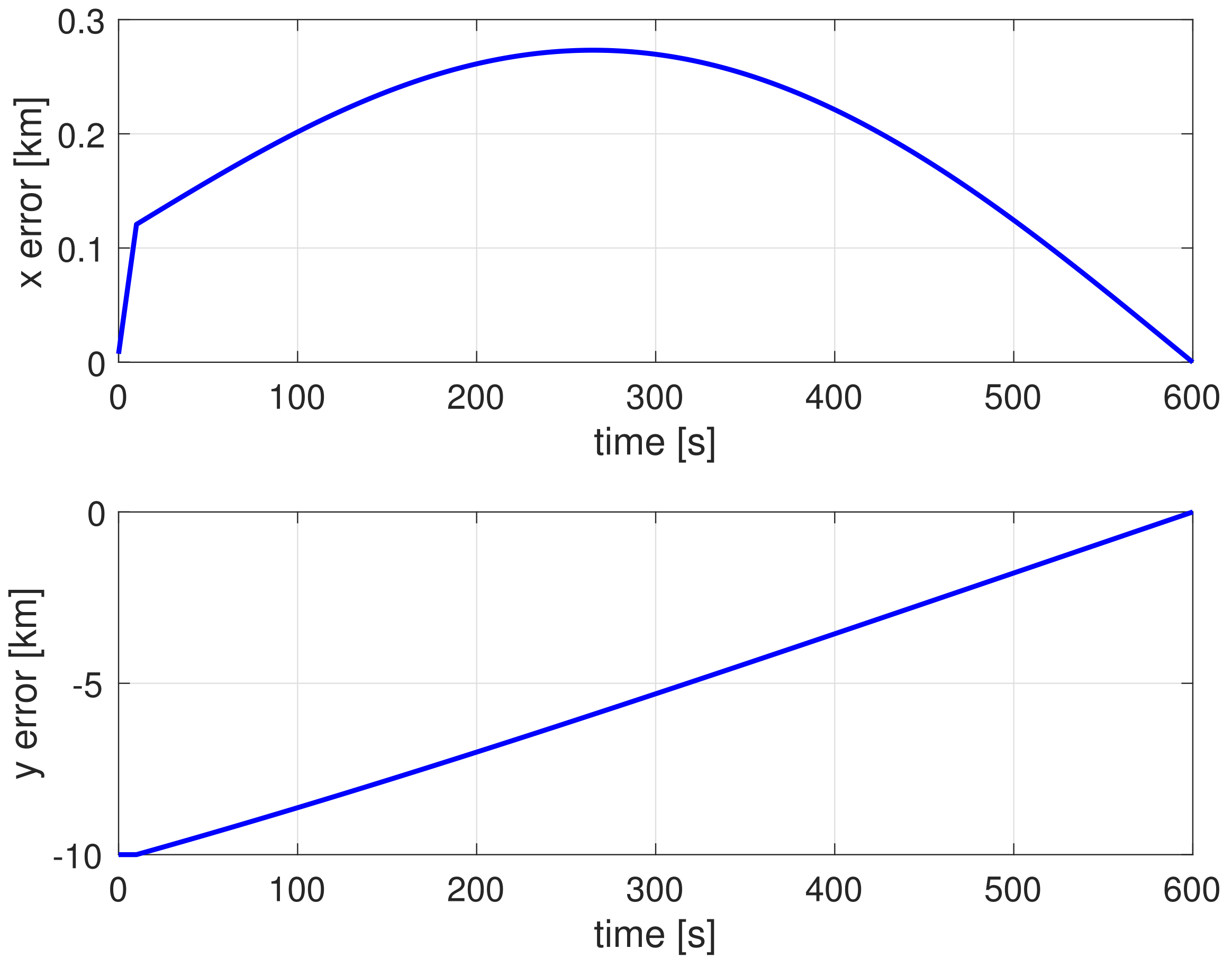
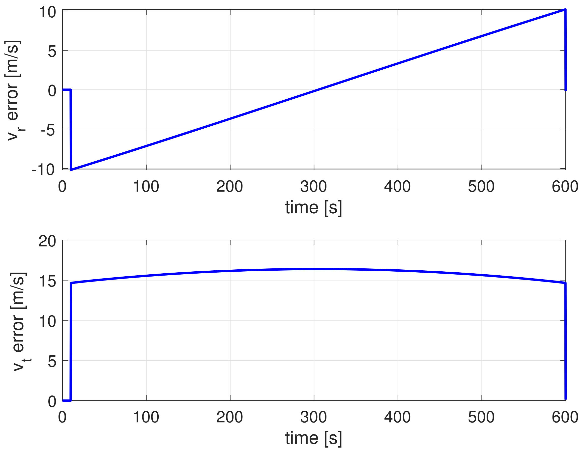
4.1. Nominal Simulation

In the nominal simulation, the guidance system is tested without the navigation solution, i.e., assuming perfect information in Equation (8). Figure 2 shows that the displacement along x and y go to zero at the end of the simulation. The obtained miss distance is indeed very small at 5 cm. It is worth noting that a distance smaller than 1 m is deemed adequate to start a docking maneuver between two small satellites [29].

The difference between the velocity of the two spacecraft is shown in Figure 3. It can be seen that the two velocities are aligned in both directions after the application of the $\delta {\mathbf{v}}_2$ command of Equation (8) at the end of the simulation. Having nulled the difference in position and velocity between the two spacecraft in the orbital plane, the nominal simulation can be, therefore, considered successful. The out-of-plane motion, in fact, is null in this case, as the considered orbits are Keplerian and no perturbations have been taken into account.

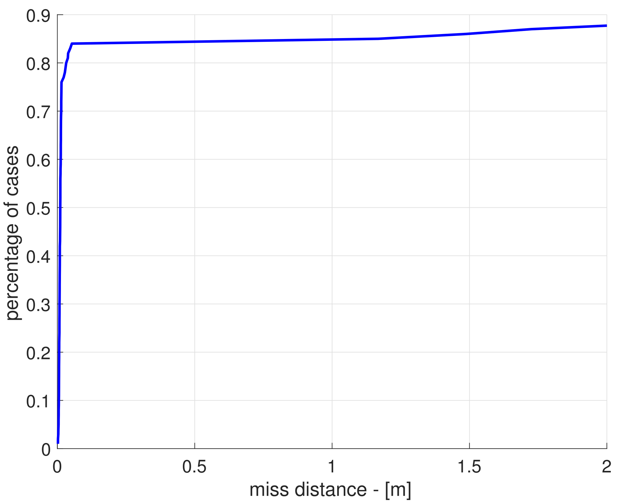
4.2. Monte Carlo Simulation

A set of 100 Monte Carlo runs has been prepared for the second simulation, varying the initial conditions ${\widehat{x}}_{0|0}\in \mathcal{N}(x_0,\sqrt{P_{0|0}})$, with $P_{0|0}$ selected as:

$$P_{0|0}=diag[{\sigma }_r^2,{\sigma }_{\xi }^2,{\sigma }_{\varphi }^2,{\sigma }_{v_r}^2,{\sigma }_{v_t}^2,{\sigma }_{v_k}^2],$$

(12)

where the variances $\sigma$ are given in Table 1.

The cumulative distribution of the miss distance obtained in the simulation campaign is shown in Figure 4. The results indicate that a miss distance shorter than 1 m is obtained in 85% of the cases, in line with the requirement on the final miss distance expressed in [29]. The accuracy obtained by the relative navigation filter in reconstructing the estimated state (9) is reported in

Table 2. Estimation accuracy.

Variable	Accuracy	Variable	Accuracy	Variable	Accuracy
r	20 m	$\xi$	0.001${}^{\circ }$	$\varphi$	0.001${}^{\circ }$
$v_r$	0.25 m/s	$v_t$	0.4 m/s	$v_k$	1 m/s

. As can be seen by comparing the values of Table 2 with the variance of the initial guess and the level of the measurement noise, the filter is able to converge to a more accurate estimate of the variable. The only variable whose estimation accuracy has not been improved by the filter is the out-of-plane component of the velocity. This can be explained by the fact that there is no out-of-plane motion of the spacecraft in this case, as the orbit is assumed totally Keplerian. Thus, the out-of-plane motion is completely unobservable and the estimate of ${\widehat{v}}_{k_T}$ remains bounded by the variance ${\sigma }_{v_k}$.

5. Conclusions

This paper has presented a guidance and navigation scheme for the rendezvous of two CubeSats. Autonomous sensing and maneuvering capabilities are becoming a requirement of many space missions, even when small satellites are employed. Therefore, it is very important to investigate algorithms that can provide the necessary GNC capabilities and to test them together in simulation so that they can be validated.

The guidance law developed for this work is an iterative algorithm that calculates a discrete firing command $\Delta v_1$ at a specific sampling time, based on the linear rendezvous theory and the HCW equations. The necessary information for the guidance law is derived from the navigation solution, which is based on a UF that processes the available on-board measurements (range and bearing).

This scheme was tested in a 3-DOF simulation in both the nominal case (perfect information) and against a Monte Carlo campaign (incomplete information), assuming values compatible with CubeSat systems and applications. The Monte Carlo simulation allows us to take into account the variations in the measurement noise and the initial guess on the target’s orbit. The results show that the obtained miss distance between the two spacecraft is below 1 m, a value suitable for the start of the docking operations.

Further work on this topic should include a trade-off study of the proposed solution against different sampling and firing times. Furthermore, the 3-DOF model should be improved to account for the main orbital perturbations, such as the Earth’s oblateness and the aerodynamic drag.

References

1. D’Amico, S.; Bodin, P.; Delpech, M.; Noteborn, R. Prisma. In Distributed Space Missions for Earth System Monitoring; Springer: Berlin/Heidelberg, Germany, 2013; pp. 599–637. [Google Scholar]
2. Gasbarri, P.; Sabatini, M.; Palmerini, G. Ground tests for vision based determination and control of formation flying spacecraft trajectories. Acta Astronaut. 2014, 102, 378–391. [Google Scholar] [CrossRef]
3. Forshaw, J.L.; Aglietti, G.S.; Navarathinam, N.; Kadhem, H.; Salmon, T.; Pisseloup, A.; Joffre, E.; Chabot, T.; Retat, I.; Axthelm, R.; et al. RemoveDEBRIS: An in-orbit active debris removal demonstration mission. Acta Astronaut. 2016, 127, 448–463. [Google Scholar] [CrossRef]
4. Prussing, J. Optimal Four-Impulse Fixed-Time Rendezvous in the Vicinity of a Circular Orbit. AIAA J. 1969, 7, 928–935. [Google Scholar] [CrossRef]
5. Prussing, J. Optimal Two- and Three-Impulse Fixed-Time Rendezvous in the Vicinity of a Circular Orbit. AIAA J. 1970, 8, 1221–1228. [Google Scholar] [CrossRef]
6. Carter, T.; Humi, M. Fuel-Optimal Maneuvers of a Spacecraft Relative to a Point in Circular Orbit. J. Guid. Control. Dyn. 1987, 10, 567–573. [Google Scholar] [CrossRef]
7. Carter, T. Fuel-Optimal Rendezvous Near a Point in General Keplerian Orbit. J. Guid. Control. Dyn. 1984, 7, 710–716. [Google Scholar] [CrossRef]
8. Pontani, M.; Conway, B. Minimum-Fuel Finite-Thrust Relative Orbit Maneuvers via Indirect Heuristic Method. J. Guid. Control. Dyn. 2015, 38, 913–924. [Google Scholar] [CrossRef]
9. Prussing, J.E.; Chiu, J.H. Optimal multiple-impulse time-fixed rendezvous between circular orbits. J. Guid. Control. Dyn. 1986, 9, 17–22. [Google Scholar] [CrossRef]
10. Pontani, M.; Ghosh, P.; Conway, B.A. Particle swarm optimization of multiple-burn rendezvous trajectories. J. Guid. Control. Dyn. 2012, 35, 1192–1207. [Google Scholar] [CrossRef]
11. Hablani, H.B.; Tapper, M.L.; Dana-Bashian, D.J. Guidance and relative navigation for autonomous rendezvous in a circular orbit. J. Guid. Control. Dyn. 2002, 25, 553–562. [Google Scholar] [CrossRef]
12. Machuca, P.; Sánchez, J.P. CubeSat Autonomous Navigation and Guidance for Low-Cost Asteroid Flyby Missions. J. Spacecr. Rocket. 2021, 58, 1858–1875. [Google Scholar] [CrossRef]
13. Pirat, C.; Ankersen, F.; Walker, R.; Gass, V. H and μ-Synthesis for Nanosatellites Rendezvous and Docking. IEEE Trans. Control. Syst. Technol. 2019, 28, 1050–1057. [Google Scholar] [CrossRef]
14. Prussing, J.E.; Conway, B.A. Orbital Mechanics; Oxford University Press: Oxford, UK, 1993. [Google Scholar]
15. Pirat, C.; Ankersen, F.; Walker, R.; Gass, V. Vision based navigation for autonomous cooperative docking of CubeSats. Acta Astronaut. 2018, 146, 418–434. [Google Scholar] [CrossRef]
16. Segal, S.; Carmi, A.; Gurfil, P. Stereovision-based estimation of relative dynamics between noncooperative satellites: Theory and experiments. IEEE Trans. Control. Syst. Technol. 2013, 22, 568–584. [Google Scholar] [CrossRef]
17. Woffinden, D.C.; Geller, D.K. Observability criteria for angles-only navigation. IEEE Trans. Aerosp. Electron. Syst. 2009, 45, 1194–1208. [Google Scholar] [CrossRef]
18. Battistini, S.; Shima, T. Differential games missile guidance with bearings-only measurements. IEEE Trans. Aerosp. Electron. Syst. 2014, 50, 2906–2915. [Google Scholar] [CrossRef]
19. Mok, S.H.; Pi, J.; Bang, H. One-step rendezvous guidance for improving observability in bearings-only navigation. Adv. Space Res. 2020, 66, 2689–2702. [Google Scholar] [CrossRef]
20. Geller, D.K.; Klein, I. Angles-only navigation state observability during orbital proximity operations. J. Guid. Control. Dyn. 2014, 37, 1976–1983. [Google Scholar] [CrossRef]
21. Cassinis, L.P.; Fonod, R.; Gill, E. Review of the robustness and applicability of monocular pose estimation systems for relative navigation with an uncooperative spacecraft. Prog. Aerosp. Sci. 2019, 110, 100548. [Google Scholar] [CrossRef]
22. Ferrari, F.; Franzese, V.; Pugliatti, M.; Giordano, C.; Topputo, F. Preliminary mission profile of Hera’s Milani CubeSat. Adv. Space Res. 2021, 67, 2010–2029. [Google Scholar] [CrossRef]
23. Cavenago, F.; Di Lizia, P.; Massari, M.; Wittig, A. On-board spacecraft relative pose estimation with high-order extended Kalman filter. Acta Astronaut. 2019, 158, 55–67. [Google Scholar] [CrossRef]
24. Fraser, C.T.; Ulrich, S. Adaptive extended Kalman filtering strategies for spacecraft formation relative navigation. Acta Astronaut. 2021, 178, 700–721. [Google Scholar] [CrossRef]
25. Battistini, S.; Cappelletti, C.; Graziani, F. Results of the attitude reconstruction for the UniSat-6 microsatellite using in-orbit data. Acta Astronaut. 2016, 127, 87–94. [Google Scholar] [CrossRef]
26. Tang, X.; Yan, J.; Zhong, D. Square-root sigma-point Kalman filtering for spacecraft relative navigation. Acta Astronaut. 2010, 66, 704–713. [Google Scholar] [CrossRef]
27. Menegaz, H.M.; Ishihara, J.Y.; Borges, G.A.; Vargas, A.N. A systematization of the unscented Kalman filter theory. IEEE Trans. Autom. Control. 2015, 60, 2583–2598. [Google Scholar] [CrossRef]
28. Wan, E.A.; Van Der Merwe, R. The unscented Kalman filter. In Kalman Filtering and Neural Networks; Wiley: Hoboken, NJ, USA, 2001; pp. 221–280. [Google Scholar]
29. Branz, F.; Olivieri, L.; Sansone, F.; Francesconi, A. Miniature docking mechanism for CubeSats. Acta Astronaut. 2020, 176, 510–519. [Google Scholar] [CrossRef]
Figure 1. Representation of the inertial and moving frames.
Applsci 12 09250 g001
Figure 2. Position errors in the x and y directions.
Applsci 12 09250 g002
Figure 3. Velocity errors in the radial and transversal directions.
Applsci 12 09250 g003
Figure 4. Miss distance cumulative distribution obtained in the simulation campaign.
Applsci 12 09250 g004