A Maximum Power Point Tracking Control Method Based on Rotor Speed PDF Shape for Wind Turbines

Abstract

Maximum power point tracking (MPPT) is the key to improve the conversion efficiency of wind energy. Concerning the current research on the MPPT control, based on the accurate tracking of rotor speed probability density function (PDF) shape for wind turbines, a novel MPPT algorithm was introduced in detail to improve the power capture and reduce mechanical damage for wind turbines. Considering the influence of wind speed distribution on the wind power generation system performance, this paper expounds a PDF shape control method of a stochastic system based on the Fokker–Planck–Kolmogorov (FPK) equation. Combining the conventional optimal torque (OT) control algorithm with the FPK equation solved by linear least-square (LLS) method, the novel MPPT control law is designed to make the PDF shape of rotor speed track the desired PDF shape as accurately as possible. The simulation verification of the novel MPPT method is carried out in the 1.5 MW wind turbine system. The results reveal that the novel MPPT method can improve the conversion efficiency of wind energy, reduce the frequent fluctuations of system variables, and significantly optimize the performance of wind power generation system.

1. Introduction

As a green renewable clean energy, wind power has attracted much attention, and its conversion has been widely concerned in recent decades [1,2]. The acquisition of more wind energy not only needs to improve the mechanical characteristics of wind turbines but also needs to continuously optimize the control method. The strategy to improve its power coefficient ($C_p$) or achieve power close to its maximum value is known as maximum power point tracking (MPPT). However, with the continuous large-scale development of wind turbines, the slow motion caused by the large inertia and the nonlinearity of wind turbine make it more and more difficult for the wind turbine to respond to the stochastic wind timely and accurately. Therefore, it is of great significance to study how to better improve the conversion efficiency of wind energy based on the dynamic tracking process and wind speed distribution characteristics.

Most of the reported MPPT algorithms in general fall into three major categories, namely, tip speed ratio (TSR) algorithm, hill-climbing search (HCS)/perturb and observe (P&O) algorithm, and optimal torque (OT)/power signal feedback (PSF) algorithm [3]. The OT algorithm focused on this paper is often used in engineering practice because of its simplicity and practicality. To make full use of wind energy, many scholars have conducted in-depth studies on the application of OT control [4,5,6]. Leithead et al. [7] added a correction component of generator torque to accelerate the transient response of wind turbines considering the influence of acceleration torque term on tracking effect. Kim et al. [8] estimated the turbine aerodynamic torque on the premise of centralized single mass transmission system. Based on the previous research, Kalyan et al. [9] proposed two improved MPPT methods based on the double-mass flexible-shaft drive train. However, most reported improvements focus on the tracking of precise operating points, ignoring the influence of wind speed distribution characteristics. For wind turbines, especially large inertia turbines, the current MPPT control methods cannot guarantee the effective tracking of any wind speed, i.e., these methods cannot guarantee the real-time and accurate tracking of the optimal tip speed ratio. Even in some cases, it may lead to an additional energy extraction from the power grid to achieve good tracking, which violates the fundamental purpose of wind turbine control.

In wind power generation system, the random wind speed will increase the difficulty of the stochastic control. Since Wang et al. [10] introduced the probability density function (PDF) into the field of stochastic control, PDF shape control has been widely used. PDF control method emphasizes that the controller is designed by tracking the desired PDF shape. The application of introducing PDF shape control theory into MPPT control can not only avoid the shortcomings of blind tracking, but also consider the wind speed distribution characteristics. At present, the Fokker–Planck–Kolmogorov (FPK) equation [11] is the most advantageous method to study the PDF shape control of nonlinear stochastic systems. Some related control designs in wind power generation system have been proposed. Zhang et al. [12] proposed that PDF controller should be designed by the error between output and optimal turbine rotor speed, that is, by controlling the PDF shape of tracking error to present a narrow distribution. This method can ensure that the system tracking error is gradually reduced and finally stabilized near zero, to achieve the output distribution control of maximum wind energy tracking. Yang et al. [13] proposed a PDF adjustment algorithm to obtain the adjustment gain of the system controller by solving the FPK equation. Although several design methods [14,15] to solve FPK equation have been provided, few scholars have paid attention to the PDF control applied to the application of PDF control in wind turbine control. In these studies of the proposed algorithm designs, the verification of control algorithm usually requires appropriate simulation and analysis on the established wind turbine model. The specific application environment should be fully considered in the establishment of wind turbine model. For example, the floating wind turbine, as a new concept wind turbine, is modeled by analytically calculating the forces operating on the system, such as buoyancy force, drag force, air thrust, drag force, and cable drag force [16]. To reduce the difficulty of modeling and focus on the comparison and analysis of control algorithms, a simplified mechanical dynamic model of wind turbine considering only stochastic wind is adopted in this paper.

The improvement of conventional OT algorithm is usually achieved by adding additional torque. This paper, firstly, presents a PDF control with full consideration of wind speed distribution characteristics. This PDF control is achieved by using linear least-square (LLS) method to solve FPK equation and can accurately track the desired turbine rotor speed. Secondly, a nonlinear MPPT optimal control design, completed by creatively introducing PDF shape control into OT control, will improve the dynamic performance of the wind turbine while playing the strengths of PDF control. This design can control the wind turbine to capture more wind energy while reducing the fluctuation of system variables, which would be verified by simulating the operation of turbulent wind speed in a 1.5 MW wind turbine.

2. Principle of MPPT Control

Figure 1 illustrates the schematic diagram of the direct-drive wind energy conversion system. In this system, the prime mover is connected to the shaft of the wind generator’s rotor, whereas the stator is linked in either case to the utility grid or standalone loads by a suitable power electronic interface. The MPPT signal is controlled by the wind power generation control system.

The wind turbine converts wind energy into mechanical energy and then generates electric energy through the operation of generators. The energy conversion of the former can be realized by the dynamic model of the wind turbine drivetrain, which can be modeled as the two-mass model, as shown in Figure 2. In this simplified mechanical dynamic model, the individual lumped inertia of the wind wheel and the generator is considered, but the damping of the drive shaft is ignored.

The shafting dynamic model of wind turbines is simplified as follows:

$$T_t-T_g=J_t\frac{d{\omega }_t}{dt}+J_g\frac{d{\omega }_g}{dt}$$

(1)

This is actually a linear combination of the acceleration at the wind wheel end and generator end. In large-scale wind turbines, the rotational inertia of the generator is much smaller than that of the wind wheel, and the stiffness of the transmission shaft is extremely large. Thus, the shafting dynamic model can be further written as follows:

$$T_t-T_g=J\frac{d{\omega }_t}{dt}$$

(2)

where $J$ is the equivalent moment of inertia of the wind turbine and $J=J_t+J_g$.

According to aerodynamic analysis, the mechanical power ($P_t$) captured by the wind turbine from the wind energy is:

$$P_t=0.5\rho \pi R^2{v}^3{C}_p\left(\lambda ,\beta \right)$$

(3)

where $\rho$ is the air density, $R$ is the radius of the wind wheel, $v$ is the incoming wind speed, and $C_p$ is the power coefficient of the wind turbine, which is determined jointly by the blade tip speed ratio ($\lambda$) and pitch angle ($\beta$). The tip speed ratio is an important parameter affecting blade performance, which is defined as the ratio of the linear velocity of the blade tip to the incoming wind speed, namely:

$$\lambda =\frac{{\omega }_{t}R}{v} .$$

(4)

So, the mechanical torque of wind turbines can be expressed:

$$T_t=\frac{P_t}{{\omega }_t}=0.5\rho C_p\left(\lambda ,\beta \right)\pi R^5\frac{1}{{\lambda }^3}{\omega }_t{}^2.$$

(5)

Generally, $C_p$ is considered a nonlinear function of $\lambda$ and $\beta$, which is calculated by empirical formula [17,18]:

$$\{\begin{array}{c}{C}_p(\lambda ,\beta )=c_1\left(\frac{c_2}{{\lambda }_i}-c_3\beta -c_4{\beta }^{c_5}-c_6\right)e^{\frac{c_7}{{\lambda }_i}}\hfill \\ \frac{1}{{\lambda }_i}=\frac{1}{\lambda +c_8\beta }-\frac{c_9}{{\beta }^3+1}\hfill \end{array}$$

(6)

where the coefficients ($c_1,c_2,\cdots ,c_9$) are related to the rotor type of wind turbines.

When the wind speed changes, MPPT control method is used to change the rotor speed of the generator by variable speed constant frequency devices, so that the wind turbine keeps running at the optimal tip speed ratio (${\lambda }_{opt}$). That is, $C_p$ is always maintained at or close to its maximum value ($C_{pmax}$) to capture more energy.

The OT control method [19] maintains a specific relationship between electromagnetic torque and rotational speed according to the curve of “$T_t-{\omega }_t$” so that the rotor speed tends to its optimal value. When the wind turbine runs at ${\lambda }_{opt}$, the power coefficient is $C_{pmax}$. Thus, the optimal power can be calculated by:

$$\{\begin{array}{c}{P}_{topt}=K_{opt}{\omega }_t{}^3 \\ K_{opt}=0.5\rho \pi R^5\frac{C_{pmax}}{{\lambda }_{opt}{}^3}.\end{array}$$

(7)

Further calculation of Equation (7) can be obtained as follows:

$$T_{topt}=K_{opt}{\omega }_t{}^2$$

(8)

where $T_{topt}$ is the optimal mechanical torque of the wind turbine and it can be obtained by measuring the experimental value of torque [20].

In the OT method, as shown in Figure 3, with the change of wind speed, the electromagnetic torque is tracked and adjusted according to its reference value ($T_g{}^{*}$), to realize the control of the wind turbine. The reference torque can be calculated as follows:

$$T_g{}^{*}=K_{opt}{\omega }_g{}^2.$$

(9)

This is the conventional OT control method, but the influence of rotor dynamic characteristics and wind speed distribution characteristics is not fully considered, so the dynamic energy capture efficiency is low. Therefore, the MPPT control strategy needs to be optimized to improve the dynamic response performance and overall wind energy capture efficiency of the wind turbine system.

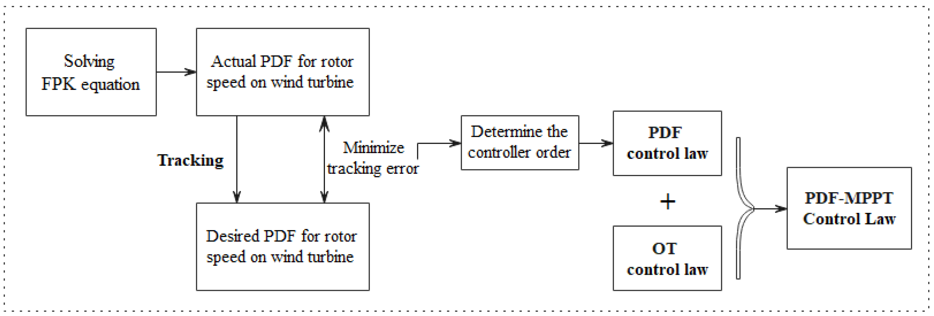
3. MPPT Control Based on PDF Shape

At present, in terms of controller design, research on maximum wind energy tracking focuses on advanced control strategies, mainly including neural network control algorithm [22], adaptive control algorithm [23], predictive control algorithm [24], sliding mode control algorithm [25,26], fuzzy logic control algorithm [27], and robust control [28]. However, due to the randomness of wind speed and the multi-variable, large inertia and nonlinear of wind turbines, the system has high requirements for control effect. Therefore, this output PDF shape control algorithm is very necessary to achieve high precision control and effectively solve the non-Gaussian problem caused by dynamic random variables. FPK equation is suitable for strong and weak non-linear systems, which is the most advantageous method to study the PDF shape control of nonlinear stochastic systems. In this PDF control algorithm based on the FPK equation, the PDF of rotor speed is selected as the output distribution. By controlling the input of the system, the output PDF shape can track the desired PDF shape, thus effectively solving the MPPT control problem caused by stochastic wind speed [29,30].

The design of MPPT control based on the PDF shape of rotor speed is shown in Figure 4. This novel MPPT control method of combining OT control and PDF shape control is marked as “PDF-MPPT control” in subsequent parts.

3.1. PDF Control Based on FPK Equation

For one-dimensional controlled nonlinear stochastic system, according to Ito’s lemma, its dynamic equation can be expressed as:

$$\dot{x}\left(t\right)=\phi \left(x\right)+G\left(x\right)\epsilon \left(t\right),\left(x\left(t_0\right)=x_0,t\in \left[t_0,T\right]\right)$$

(10)

where $x\left(t\right)$ is the system status variable and has an initial state $x\left(t_0\right)$, $\phi \left(x\right)$ is the nonlinear function of system state, $G\left(x\right)$ is the diffusion coefficient and $\epsilon \left(t\right)$ is the stochastic input vector or interference vector of the system. The correlation coefficient matrix of $\epsilon \left(t\right)$ is $E\left\{\epsilon \left(t\right)\epsilon \left(t^{\prime }\right)\right\}=2\pi S_{\epsilon 1}\delta \left(t-t^{\prime }\right)$, where $S_{\epsilon 1}$ is the power spectral density of $\epsilon \left(t\right)$ and often take constant value.

The polynomial nonlinear system is the most common system type. For this kind of system, $\phi \left(x\right)$ is calculated by:

$$\phi \left(x\right)=F\left(x\right)+u\left(x\right)$$

(11)

where $u\left(x\right)$ is the control function to be obtained and $F\left(x\right)$ is the nonlinear part of the system.

Thus, a PDF controller in nonlinear form can be designed:

$$\begin{array}{cc}\hfill u\left(x\right)& =\underset{\phi \left(x\right)}{\underbrace{b_l{x}^l+b_{l-1}{x}^{l-1}+\cdots +b_{1}x+b_0}}-\underset{F\left(x\right)}{\underbrace{\left(a_r{x}^r+a_{r-1}{x}^{r-1}+\cdots +a_{1}x+a_0\right)}}\hfill \\ \hfill & =b_l{x}^l+b_{l-1}{x}^{l-1}+\cdots +\left(b_r-a_r\right)x^r+\left(b_{r-1}-a_{r-1}\right)x^{r-1}+\cdots +\left(b_1-a_1\right)+\left(b_0-a_0\right)\hfill \end{array}$$

(12)

where $b_l,b_{l-1},\cdots ,b_0$ and $a_r,a_{r-1},\cdots ,a_0$ are the coefficients, and $r\le l$.

In the system of (10), the stationary FPK equation corresponding to the PDF of the state variable is:

$$-\frac{d\left[\alpha \left(x\right)p_{trf}\left(x\right)\right]}{dx}+\frac{1}{2}\frac{d^2\left[\gamma \left(x\right)p_{trf}\left(x\right)\right]}{d{x}^2}=0$$

(13)

where $p_{trf}\left(x\right)$ is the PDF of system’s state variable, $\alpha \left(x\right)=\phi \left(x\right)$ and $\gamma \left(x\right)=2\pi S_{\epsilon 1}{G}^2\left(x\right)$.

Since the precise solution of the FPK equation is difficult to obtain, the optimal performance index can be constructed according to the distribution shape of the goal function ($p_{trf}\left(x\right)$), and the approximate solution of the FPK equation ($p_{trf}^{\approx }\left(x\right)$). Control inputs are determined by minimizing the performance index:

$$\mathit{min}e\left(l\right)={{\displaystyle \int }}_{-\infty }^{+\infty }{\left(p_{trf}\left(x\right)-p_{trf}^{\approx }\left(x\right)\right)}^{2}dx$$

(14)

where $e\left(l\right)$ is the system tracking error of $l$-order controller.

For simple calculation, let $S_{\epsilon 1}=\frac{1}{\pi }$. Then, the FPK equation corresponding to $p_{trf}^{\approx }\left(x\right)$ is:

$$-\frac{d\left[\phi \left(x\right)p_{trf}^{\approx }\left(x\right)\right]}{dx}+\frac{d^2\left[G{\left(x\right)}^2{p}_{trf}^{\approx }\left(x\right)\right]}{d{x}^2}=0.$$

(15)

When $G\left(x\right)=1$, the above FPK equation is transformed into the following second-order homogeneous differential equation:

$$p_{trf}^{\approx }{}^{″}\left(x\right)-{\phi }^{\prime }\left(x\right)p_{trf}^{\approx }\left(x\right)-\phi \left(x\right)p_{trf}^{\approx }{}^{\prime }\left(x\right)=0.$$

(16)

Assuming that one of the special solutions of $p_{trf}^{\approx }\left(x\right)$ is $p_1\left(x\right)=e^{q\left(x\right)}$ and considering $e^{q\left(x\right)}\ne 0$, the following equation is obtained by substituting $p_1\left(x\right)$ into Equation (16):

$$q^{″}\left(x\right)+{\left(q^{\prime }\left(x\right)\right)}^2-\phi \left(x\right)q^{\prime }\left(x\right)-{\phi }^{\prime }\left(x\right)=0.$$

(17)

Similarly, when another special solution of $p_{trf}^{\approx }\left(x\right)$ is $p_2\left(x\right)=c\left(x\right)e^{q\left(x\right)}$ and $c\left(x\right)\ne 0$, there is:

$$c^{″}\left(x\right)+\left[2q^{\prime }\left(x\right)-\phi \left(x\right)\right]c^{\prime }\left(x\right)=0.$$

(18)

Solving Equation (17) and Equation (18) respectively to obtain the unknown variables in $p_1\left(x\right)$ or $p_2\left(x\right)$:

$$\{\begin{array}{c}q\left(x\right)={\displaystyle \int }\phi \left(x\right)dx \\ c\left(x\right)={\displaystyle \int }{e}^{\int \left(\phi \left(x\right)-2q^{\prime }\left(x\right)\right)dx}dx.\end{array}$$

(19)

Since $c^{\prime }\left(x\right)=e^{\int \left(\phi \left(x\right)-2q^{\prime }\left(x\right)\right)dx}\ne 0$, $p_1\left(x\right)$ and $p_2\left(x\right)$ are linearly independent, thus the general solution of Equation (16) is:

$$p_{trf}^{\approx }\left(x\right)=c_{p1}{p}_1\left(x\right)+c_{p2}{p}_2\left(x\right)=c_{p1}{e}^{\int \phi \left(x\right)dx}+c_{p2}{e}^{\int \phi \left(x\right)dx}{\displaystyle \int }{e}^{-\int \left(x\right)dx}dx.$$

(20)

The approximate solution of FPK equation can be obtained either by $c_{p1}=0$ or $c_{p2}=0$.

When $c_{p2}=0$ and $c_{p1}$ meets the normalization condition, $c_{p1}=\frac{1}{\left({\displaystyle \int }{e}^{\int \phi \left(x\right)dx}dx\right)}$, the $p_{trf}^{\approx }\left(x\right)$ of that FPK equation can be expressed as:

$$\begin{array}{cc}\hfill p_{trf}^{\approx }\left(x\right)& =c_{p1}\mathit{exp}\left(\frac{1}{l+1}{b}_l{x}^{l+1}+\frac{1}{l}{b}_{l-1}{x}^l+\cdots +\frac{1}{2}{b}_1{x}^2+b_{0}x+c_0\right)\hfill \\ & =c_{p1}\mathit{exp}\left({\displaystyle {\displaystyle \sum }_{i=0}^{1+1}}{c}_i{x}^i\right)\hfill \end{array}$$

(21)

where $c_0$ is an arbitrary constant and the exponential term coefficient is $c_i=\frac{b_{i-1}}{i} \left(i\ge 1\right)$.

The LLS method is used to determine unknown coefficients, so as to obtain the PDF control law.

(1). If $N+1$ points are randomly generated in the value domain of $x$, there will be $N+1$ equations about $x$:

$${\displaystyle \sum }_{i=0}^{1+1}{c}_i{x}^i=\mathit{ln}\frac{p_{trf}^{\approx }\left(x_j\right)}{c_{p1}},j=0,1,2,\cdots ,N.$$

(22)

(2). Consider that $p_{trf}^{\approx }\left(x_j\right)$ is replaced by the sum of the desired PDF and the equation error term, then the solving equation of the PDF control law can be converted into:

$${\displaystyle \sum }_{i=0}^{1+1}{c}_i{x}^i=\mathit{ln}\frac{p_{trf}\left(x_j\right)}{c_{p1}}-e_i\left(x_j\right),j=0,1,2,\cdots ,N$$

(23)

where $p_{trf}\left(x_j\right)$ is the desired PDF of state variable and $e_i\left(x_j\right)$ is the error term of the equation.

(3). The experimental data set, ${\left\{x_j,\mathit{ln}\left(\frac{p_{trf}\left(x_j\right)}{c_{p1}}\right)\right\}}_{j=0~N}$, is established according to the desired PDF, and $c_i$ can be obtained by substituting them into Equation (23). In addition, the appropriate controller can be determined by the tracking error, $e\left(l\right)$, between the desired PDF and the approximate solution of the FPK equation.

(4). The gain of $\phi \left(x\right)$ can be determined by $b_i=\left(i+1\right)c_{i+1}\left(i=0,1,\cdots ,l\right)$, and the final PDF control law can be determined according to Equation (12):

$$u\left(x\right)={\displaystyle \sum }_{i=0}^r\left(\left(i+1\right)c_{i+1}-a_i\right)x^i-{\displaystyle \sum }_{i=r+1}^l\left(i+1\right)c_{i+1}{x}^i.$$

(24)

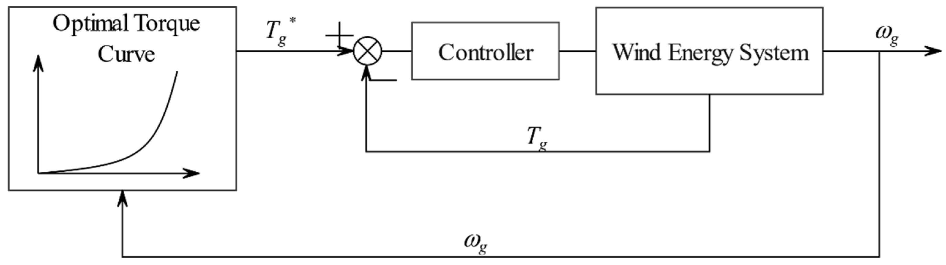
3.2. OT Control Based on PDF Shape

According to the principle of maximum wind energy capture, the capture of more wind energy is achieved by changing the rotor speed of the generator to keep the wind turbine working at ${\lambda }_{opt}$. Therefore, the optimal rotor speed of the wind turbine (${\omega }_t{}_{opt}$) is selected as the tracking goal, the actual ${\omega }_t$ is selected as the system output, and the electromagnetic torque ($T_g$) of the generator is used as the controller output. Ignoring the tracking error between $T_g$ and $T_g{}^{*}$, let $x\left(t\right)={\omega }_t\left(t\right)$, $y\left(t\right)={\omega }_t\left(t\right)$, $u\left(x\right)=T_g$, and the state equation of wind power generation system is established as follows:

$$\{\begin{array}{c}\frac{dx\left(t\right)}{dt}=\frac{\rho \pi R^5}{2J}\frac{C_T\left(\lambda ,\beta \right)}{{\lambda }^2}{x}^2\left(t\right)-\frac{1}{J}u\left(x\right)+\epsilon \left(t\right)\hfill \\ y\left(t\right)=x\left(t\right) \end{array}$$

(25)

where $\epsilon \left(t\right)$ is the interference caused by wind speed uncertainty and other random factors during operation.

If Equation (25) is written in the form of Equation (12), the partial coefficients of the controller:

$$a_0=a_1=0,a_2=\frac{\rho \pi R^5}{2J}\frac{C_T\left(\lambda ,\beta \right)}{{\lambda }^2},a_3=a_4=\cdots =a_r=0.$$

(26)

Due to the large stiffness of the transmission shaft, ${\omega }_t={\omega }_g$ is the default. The controller gain of the system is produced by Equations (24) and (25), which is:

$$u\left(x\right)=J\left\{-c_1{\omega }_g+\left(\frac{\rho \pi R^5{C}_T\left(\stackrel{\wedge }{\lambda },\beta \right)}{2J{\stackrel{\wedge }{\lambda }}^2}-2c_2\right){\omega }_g{}^2-3c_3{\omega }_g{}^3-\cdots -\left(l+1\right)c_{l+1}{\omega }_g{}^l\right\}$$

(27)

where $C_T(\stackrel{\wedge }{\lambda },\beta )$. is the estimated value of aerodynamic torque coefficient, and $C_T(\stackrel{\wedge }{\lambda },\beta )=C_p(\stackrel{\wedge }{\lambda },\beta )/\stackrel{\wedge }{\lambda }$. In addition, $dx\left(t\right)/dt<0$ can be obtained by substituting Equation (27) into the first-order inertial system of (25), so the stability of the system can be guaranteed, and the convergence of OT method is also verified.

In the actual control operation, the calculation of some variables is usually replaced by estimated values. Thus, Equation (27) is converted to the following:

$$\{\begin{array}{c}u\left(x\right)={\stackrel{\wedge }{T}}_t-J{\displaystyle {\displaystyle \sum }_{i=0}^l}\left(i+1\right)c_{i+1}{\omega }_g{}^i\\ {\stackrel{\wedge }{T}}_t=\frac{\rho \pi R^5{C}_T\left(\stackrel{\wedge }{\lambda },\beta \right)}{2{\stackrel{\wedge }{\lambda }}^2}{\omega }_g{}^2 . \end{array}$$

(28)

When the wind turbine system runs in a steady state, it works under the optimal blade tip ratio, that is, ${\stackrel{\wedge }{T}}_t=T_g{}^{*}=K_{opt}{\omega }_g{}^2$. The $T_g{}^{*}$ of the wind turbine system can be determined as follows:

$$T_g{}^{*}=K_{opt}{\omega }_g{}^2-J{\displaystyle \sum }_{i=0}^l\left(i+1\right)c_{i+1}{\omega }_g{}^i.$$

(29)

This design still focuses on tracking the maximum power point (MPP), but also takes into account the stochastic distribution of wind speed. This novel control design can track the goal in a small range instead of tracking a certain point, avoiding the damage to the system caused by frequent fluctuation of rotor speed.

4. Simulation and Results

To further verify the control effect of the controller designed in the above section and its influence on the wind energy capture performance of the system, a test simulation was carried out through the 1.5 MW permanent magnet synchronous generator (PMSG) wind turbine system model in MATLAB/Simulink. The specific simulation model parameters are shown in

Table 1. Parameters of the 1.5 MW wind turbine system.

Name	Symbol	Value	Unit
Rotor radius	$R$	33.05	m
Stiffness of rotor	$K_s$	48,376	N·m/rad
The moment inertia of rotor	$J$	35,000	kg·m2
nominal voltage	$U_{nom}$	575	V
nominal frequency	$f_{nom}$	60	Hz
Number of poles	$p_n$	48
Stator resistance	$R_s$	0.027	pu
Stator inductance	$L_d,L_q$	0.5131	pu
Flux induced by magnets	${\psi }_f$	1.18842	pu
Air density	$\rho$	1.12	kg/m3
Rated power	$P_{rate}$	1.5	MW
Rated wind speed	$v_{rate}$	12.1	rad/s
Rated rotor speed	${\omega }_{rrate}$	1.1	rad/s
Pitch angle	$\beta$	0	${}^{\circ }$
Optimum TSR	${\lambda }_{opt}$	10.5
Maximum power coefficient	$C_{pmax}$	0.44

.

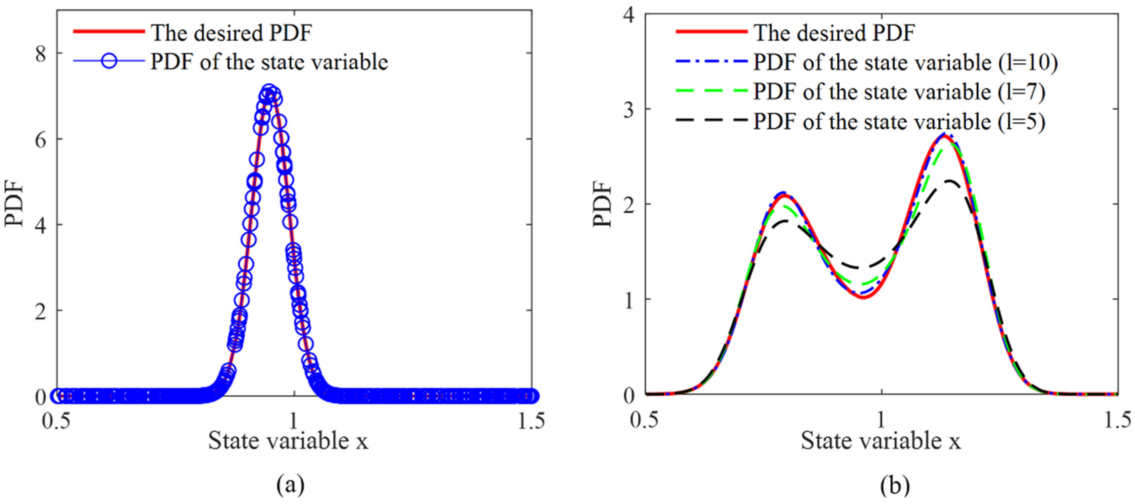
4.1. Controller Determination

For different conditions of whether the average wind speed changes or not, wind samples whose desired rotor speed PDF obeys unimodal Gaussian distribution and variable weight multi-Gaussian distribution are selected for simulation. It is necessary to determine the order of the controller applied under the two distributions according to the effect of PDF shape tracking to carry out the corresponding control design.

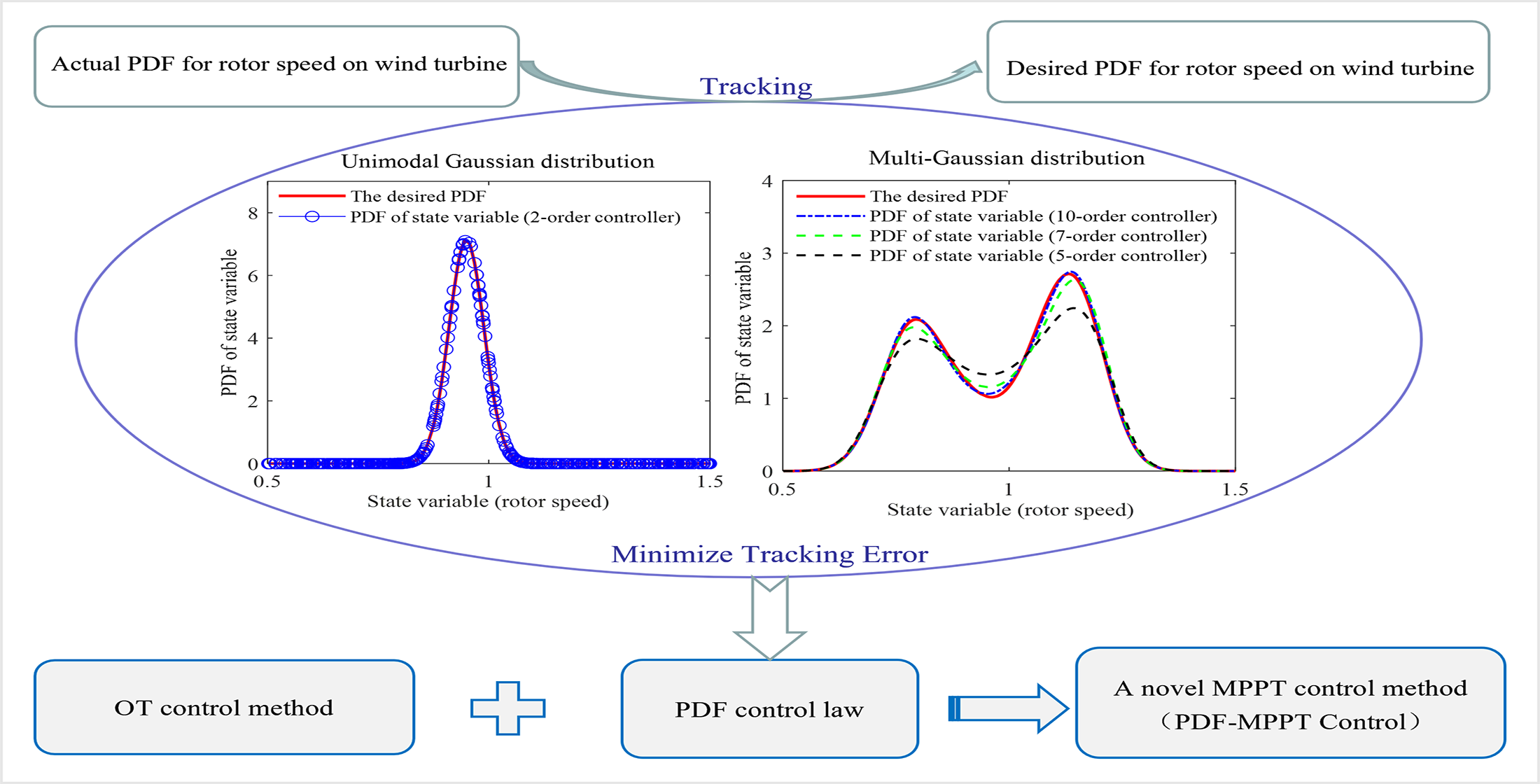
4.1.1. Goal PDF Is Gaussian Distribution

The control design is carried out considering that the desired rotor speed PDF obeys the unimodal Gaussian distribution. The goal PDF expression is:

$$p_{trf}\left(x\right)=\frac{1}{\sqrt{2\pi }\sigma }\mathit{exp}\left(-\frac{{\left(x-\mu \right)}^2}{{\sigma }^2}\right)$$

(30)

where $\mu =0.9495$ and $\sigma =0.056$.

According to the controller design principle and method described in Section 3.1, the polynomial in Equation (24) is fitted with different orders. When the order of the controller is taken as two, the tracking effect of rotor speed PDF shape is shown in Figure 5a.

It can be found that when $l=2$, the output PDF curve completely coincides with the desired PDF curve. At this time, the tracking error between the approximate solution of FPK equation and the goal PDF is $e\left(l\right)=3.4078\times {10}^{-26}$, which indicates that the tracking accuracy is very high and the tracking effect of the output PDF is very good.

The two-order controller of this system is:

$$T_g{}^{*}=K_{opt}{\omega }_g{}^2-J\left(c_1+2c_2{\omega }_g+3c_3{\omega }_g{}^2\right)$$

(31)

where $c_0$, $c_1$, $c_2$ and $c_3$ are the coefficients in the corresponding parametric set ($C_2$) and are listed in

Table A1. The coefficient set of two-order controller.

Symbol	${\mathit{C}}_2$
$c_0$	−287.830867811171
$c_1$	605.548469387750
$c_2$	−318.877551020403
$c_3$	$-1.72248700320832\times$ 10−12

in Appendix A.

4.1.2. Goal PDF Is Multi-Gaussian Distribution

The control design is carried out considering that the desired rotor speed PDF obeys the variable weight multi-Gaussian distribution. The goal PDF expression is:

$$p_{trf}\left(x\right)={\displaystyle \sum }_{z=1}^4{w}_z\mathit{exp}\left(-\frac{{\left(x-{\mu }_z\right)}^2}{{\sigma }_z{}^2}\right)$$

(32)

where the values of $w_z$, ${\mu }_z$, and ${\sigma }_z$ are shown in

Table 2. Parameters of $p_{trf}\left(x\right)$ when the goal function is multi-Gaussian distribution.

Parameter	$\mathit{z}$ = 1	$\mathit{z}$ = 2	$\mathit{z}$ = 3	$\mathit{z}$ = 4
$w_z$	1.16800	1.61300	1.89800	0.95800
${\mu }_z$	1.17100	0.77670	1.10300	0.89170
${\sigma }_z$	0.08411	0.09418	0.10170	0.12660

.

Similarly, when the order of the controller is taken as five, seven and ten, the tracking effect of rotor speed PDF shape is shown in Figure 5b.

It can be found that the tracking accuracy become increasingly higher with the increase of controller order, and the control effect improves accordingly. The specific tracking error and the unknown coefficients in $p_{trf}^{\approx }\left(x\right)$ are shown in

Table 3. Coefficients and tracking errors of controllers under multi-Gaussian distribution.

Controller Order	$\mathbf{Coefficients}\mathbf{in}{\mathit{p}}_{\mathit{t}\mathit{r}\mathit{f}}^{\approx }\left(\mathit{x}\right)$	Tracking Error
5	$C_5$	0.0342
7	$C_7$	0.0071
10	$C_{10}$	0.0010

where $C_5$, $C_7$ and $C_{10}$ respectively represent the corresponding unknown coefficient set in $p_{trf}^{\approx }\left(x\right)$ when the controller order is five, seven, and ten. Their specific values are shown in Table A2 in Appendix A.

.

Considering the high system sensitivity and difficulty of realization caused by a too large order, the seven-order controller is selected, and its control law is:

$$T_g{}^{*}=K_{opt}{\omega }_g{}^2-J\left(c_1+2c_2{\omega }_g+3c_3{\omega }_g{}^2+\cdots +8c_8{\omega }_g{}^7\right)$$

(33)

where $c_1,c_2,\cdots ,c_7 \mathrm{and} c_8$ are the coefficients of the output PDF when the seven-order controller is applied.

This design combines the OT control with the PDF control of the stochastic system, and fully considers the influence of the stochastic distribution of wind speed. The novel control design has a good tracking effect on the changing stochastic wind speed, which can effectively improve the wind energy capture efficiency of the wind turbine.

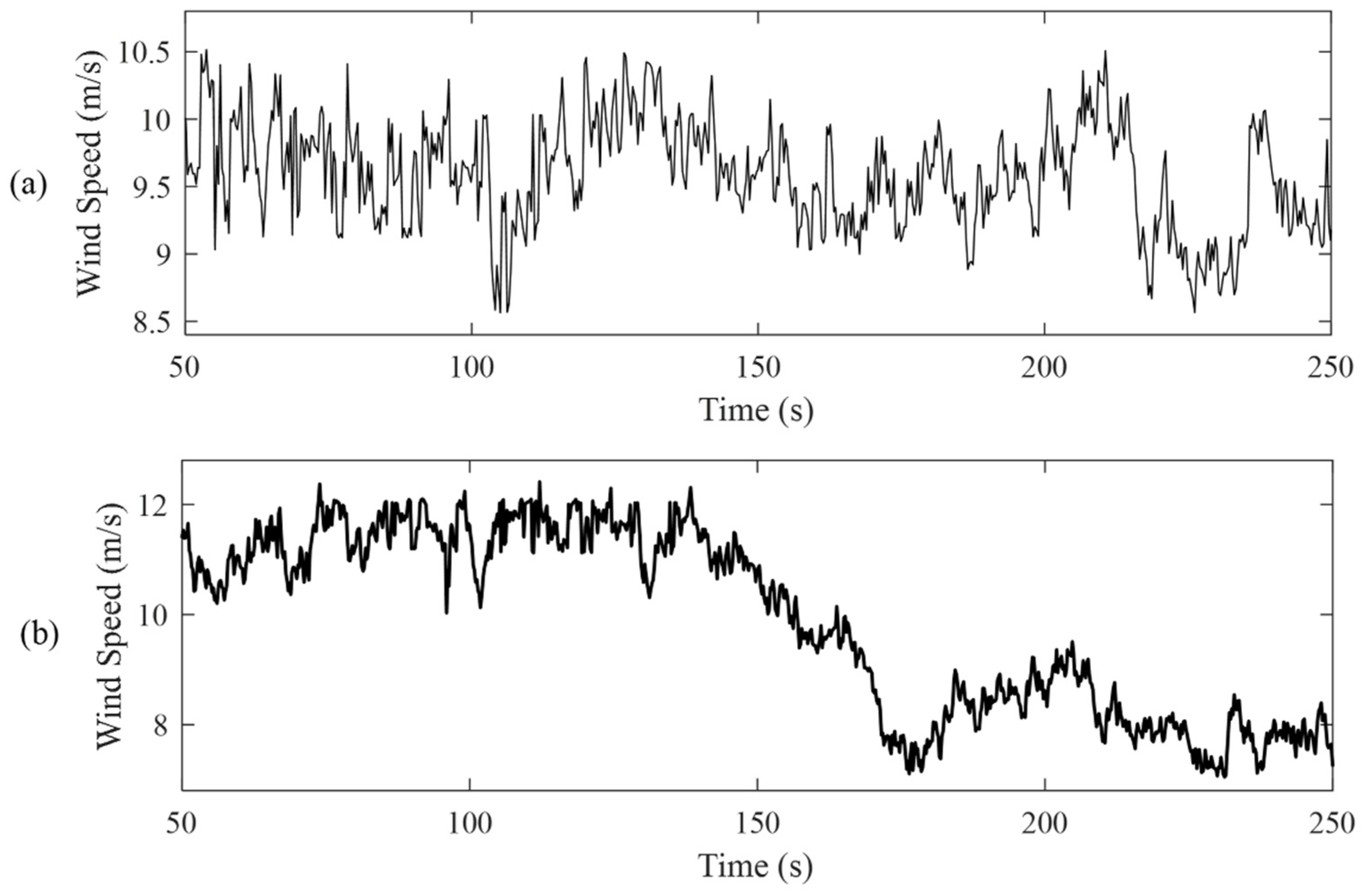
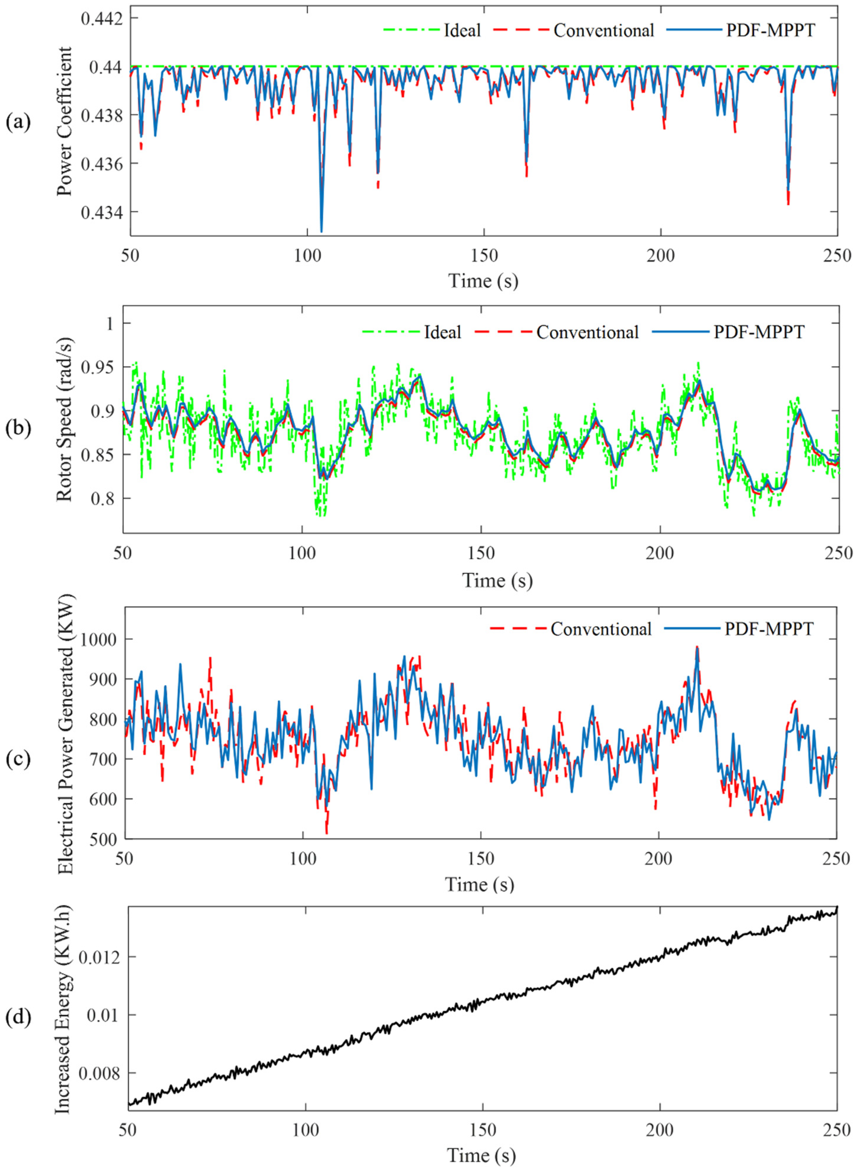
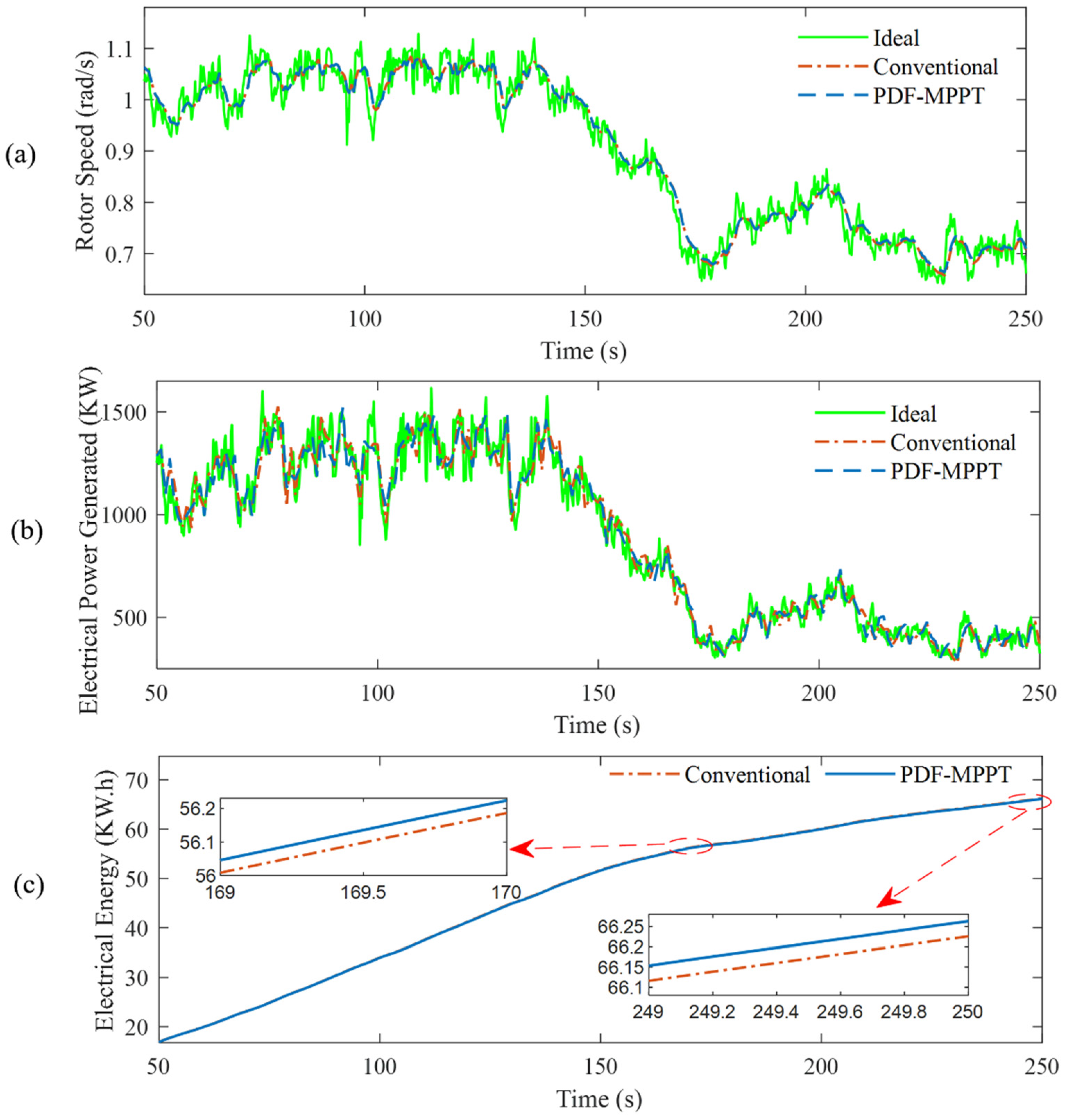
4.2. Performance Validation

For the turbulent wind speed signals as shown in Figure 6, the corresponding PDF-MPPT control is applied in the established 1.5 MW direct-drive wind power generation system and compared with the conventional OT control method named “conventional (method)” and the ideal condition named “ideal”. The novel MPPT control based on PDF control is named the “PDF-MPPT (method)”, which can be verified and analyzed by simulation results.

For the turbulent wind speed as shown in Figure 6a, the response effect can be observed by applying the 2-order control law to the wind power generation system, as shown in Figure 7.

Figure 7a shows the change of power coefficient of conventional and novel MPPT methods under the same wind condition. The power coefficient of this system controlled by the novel MPPT control method is always higher than that of the conventional MPPT control when wind speed changes, especially at high wind speeds. In addition, since wind power is not only related to $C_p$, but also specific wind speed, comprehensive factors. These comprehensive factors make novel MPPT control have better energy capture performance than conventional MPPT control.

Figure 7b describes the dynamic response of rotor speed. It can be found that when the wind speed changes too fast, novel MPPT control can make the system reduce the frequent fluctuation of rotor speed and respond to the stochastic change of wind speed more quickly. Figure 7c also shows that, compared with the conventional MPPT method, the fluctuation of the rotor speed and the electromagnetic torque under novel MPPT control is reduced. This is because the characteristic of PDF control is to reduce the fluctuation range of various variables in the system. It is this characteristic that makes novel MPPT control reduce the mechanical damage to a certain extent.

Figure 7d shows the change of cumulative power generation increment of the novel MPPT control compared with conventional MPPT control. Between 50 s and 250 s, PDF-MPPT control makes the wind energy captured by wind turbines always greater than the conventional MPPT method, which confirms the impact of that the novel MPPT method on energy improvement. This novel method can improve the power generation of the system over a while to a certain extent.

Similarly, for another turbulent wind speed shown in Figure 6b, the system response performance under the application of the 7-order control law is shown in Figure 8.

Figure 8a shows the dynamic response of rotor speed. It can be found that the difference in rotor speed response between the two MPPT control methods is not obvious. However, it can be seen from Figure 8b that the novel MPPT method reduces the fluctuation degree of electrical power generated. This indicates that the fluctuation range of each variable under the control of the novel method is small, which can reduce the mechanical damage to a certain extent. In addition, because the wind sample contains more high-frequency components, and the wind turbine tracks the change of wind speed by adjusting the rotor speed, which leads to some sharp profiles in the simulation results of Figure 8a,b, the fluctuation of rotor speed and electrical power is much weaker than that of wind speed.

Figure 8c shows the changes in cumulative power generation of the system under the conventional MPPT control and the novel MPPT control in the period of 50–250 s. Under high wind speed, as of 170 s, the cumulative power generation of the system under the two controls is 56.1863 kw·h and 56.2231 kw·h respectively. Later, when the wind speed is low, the energy capture efficiency and the corresponding cumulative power generation of the system under the novel MPPT control decreases. As of 250 s, the cumulative power generation of the system under the two controls is 66.2629 kw·h and 66.2252 kw·h respectively. It can be found that the cumulative power generation of the system controlled by the novel MPPT method is always higher than that of the conventional method, indicating that the energy accumulated at high wind speed can still make up for the energy loss at low wind speed.

The effectiveness of the novel MPPT control is verified by analyzing the changes in relevant indicators in Figure 6 and Figure 7.

5. Conclusions

The conventional MPPT method mainly focuses on the steady-state performance and ignores the dynamic characteristics of the wind turbine. At present, the proposed MPPT control method aims to accurately track the change in wind speed without considering the influence of wind speed distribution characteristics. The uncertainty of wind speed, the large inertia of the wind turbine, and the slow dynamics caused by the wind turbine system nonlinearity make it difficult for the wind turbine to respond to the high turbulence in stochastic wind timely and accurately.

To solve the problem caused by blind tracking, a novel MPPT control method is very necessary. Considering the influence of the stochastic distribution of wind speed on the system control performance, the PDF control was introduced, and a novel MPPT control design-based rotor speed PDF shape was proposed. The PDF controller is designed by solving the FPK equation with the LLS method so that the PDF shape of the system state variable can better approach the PDF shape of the goal. Combining this PDF control with the conventional OT control, the novel MPPT control for wind turbines is proposed, which can accurately track the desired PDF and improve the wind energy capture efficiency.

Simulation results of a 1.5 MW PMSG wind turbine system show that the novel MPPT control can indeed increase the power coefficient of the system under high wind speed, make the system respond to the random change of wind speed more quickly, and effectively improve the overall power generation in a period. In addition, this control method can reduce the fluctuation of rotor speed and torque as well as reduce the mechanical damage.

The novel MPPT method improves the overall power generation to a certain extent and possesses a huge reference value for the further study of the control problem of stochastic wind power generation system. Future works may include the application of B-spline modeling to design the low-order controller and the novel MPPT method in real variable-speed wind turbines.

References

1. Li, J.; Wang, G.; Li, Z.; Yang, S.; Chong, W.T.; Xiang, X. A review on development of offshore wind energy conversion system. Int. J. Energy Res. 2020, 44, 9283–9297. [Google Scholar] [CrossRef]
2. Ahmed, B.; Nurul, H.; Siti, Y.; Aisha, H.; Sheroz, K.; Alhareth, Z. Paper review: Maximum power point tracking for wind energy conversion system. In Proceedings of the 2020 2nd International Conference on Electrical, Control and Instrumentation Engineering (ICECIE), Kuala Lumpur, Malaysia, 28 November 2020; pp. 1–6. [Google Scholar]
3. Abdullah, M.A.; Yatim, A.H.M.; Tan, C.W.; Saidur, R. A review of maximum power point tracking algorithms for wind energy systems. Renew. Sustain. Energy Rev. 2012, 16, 3220–3227. [Google Scholar] [CrossRef]
4. Wang, Q.; Chang, L. An intelligent maximum power extraction algorithm for inverter-based variable speed wind turbine systems. IEEE Trans. Power Electron. 2004, 19, 1242–1249. [Google Scholar] [CrossRef]
5. Hua, G.; Geng, Y. A novel control strategy of MPPT taking dynamics of wind turbine into account. In Proceedings of the 2006 37th IEEE Power Electronics Specialists Conference, Jeju, Korea, 18–22 June 2006; pp. 1–6. [Google Scholar]
6. Barendse, P.; Naidoo, R.; Douglas, H.; Pillay, P. A new algorithm for improved dip/sag detection with application to improved performance of wind turbine generators. In Proceedings of the Conference Record of the 2006 IEEE Industry Applications Conference Forty-First IAS Annual Meeting, Tampa, FL, USA, 8–12 October 2006; pp. 118–123. [Google Scholar]
7. Leithead, W.E.; Connor, B. Control of variable speed wind turbines: Design task. Int. J. Control 2010, 73, 1189–1212. [Google Scholar] [CrossRef]
8. Kim, K.H.; Van, T.L.; Lee, D.C.; Song, S.H.; Kim, E.H. Maximum output power tracking control in variable-speed wind turbine systems considering rotor inertial power. IEEE Trans. Ind. Electron. 2013, 60, 3207–3217. [Google Scholar] [CrossRef]
9. Yenduri, K.; Sensarma, P. Maximum power point tracking of variable speed wind turbines with flexible shaft. IEEE Trans. Sustain. Energy 2016, 7, 956–965. [Google Scholar] [CrossRef]
10. Yin, S.; Yu, D.; Luo, Z.; Xia, B. Unified polynomial expansion for interval and random response analysis of uncertain structure-acoustic system with arbitrary probability distribution. Comput. Methods Appl. Mech. Eng. 2018, 336, 260–285. [Google Scholar] [CrossRef]
11. Li, F.; Liu, Y. General stochastic convergence theorem and stochastic adaptive output-feedback controller. IEEE Trans. Autom. Control 2017, 62, 2334–2349. [Google Scholar] [CrossRef]
12. Zhang, J.; Guo, P.; Zhao, J. Probability density function control for maximum wind energy tracking of variable speed wind turbine. In Proceedings of the 26th Chinese Process Control Conference (CPCC2015), Nangchang, China, 31 July–3 August 2015; p. 335. [Google Scholar]
13. Yang, H.; Fu, Y.; Qian, F. The Probability Density Function Adjust for Uncertain Stochastic Systems. In Proceedings of the 2018 37th Chinese Control Conference (CCC), Wuhan, China, 25–27 July 2018; pp. 292–296. [Google Scholar]
14. Wang, L.; Qian, F.; Liu, J. Shape control on probability density function in stochastic systems. J. Syst. Eng. Electron. 2014, 25, 144–149. [Google Scholar] [CrossRef]
15. Wang, L. Research on PDF Shape Control in Non-Linear Stochastic Systems. Ph.D. Thesis, Xi’an University of Technology, Xi’an, China, 2016. [Google Scholar]
16. Keighobadi, J.; KhalafAnsar, H.; Naseradinmousavi, P. Adaptive neural dynamic surface control for uniform energy exploitation of floating wind turbine. Appl. Energy 2022, 316, 119132. [Google Scholar] [CrossRef]
17. Fortmann, J. Modeling of Wind Turbines with Doubly Fed Generator System; Springer Fachmedien Wiesbaden: London, UK, 2015. [Google Scholar]
18. Lubosny, Z. Wind Turbine Operation in Electric Power Systems; Springer: London, UK, 2010. [Google Scholar]
19. Morimoto, S.; Nakayama, H.; Sanada, M.; Takeda, Y. Sensorless output maximization control for variable-speed wind generation system using IPMSG. IEEE Trans. Ind. Appl. 2005, 41, 60–67. [Google Scholar] [CrossRef]
20. Tan, K.; Islam, S. Optimum control strategies in energy conversion of PMSG wind turbine system without mechanical sensors. IEEE Trans. Energy Convers. 2004, 19, 392–399. [Google Scholar] [CrossRef]
21. Qi, L.; Zheng, L.; Bai, X.; Chen, Q.; Chen, Y.J.A.S. Nonlinear Maximum Power Point Tracking Control Method for Wind Turbines Considering Dynamics. Appl. Sci. 2020, 10, 811. [Google Scholar] [CrossRef] [Green Version]
22. Hao, X.; Shi, N.; Gao, C. Application of fuzzy-neural network control in wind power system. Inf. Technol. Netw. Secur. 2010, 29, 91–96. [Google Scholar]
23. Wang, T.; Li, L.; Xu, J.; Tan, J.; Wang, X. Adaptive control for the maximum power point tracking of wind energy conversion system considering torque loss. In Proceedings of the 33rd Chinese Control Conference, Nanjing, China, 28–30 July 2014; pp. 7116–7120. [Google Scholar]
24. Dang, D.Q.; Wu, S.; Wang, Y.; Cai, W. Model predictive control for maximum power capture of variable speed wind turbines. In Proceedings of the 2010 Conference Proceedings IPEC, Singapore, 27–29 October 2010; pp. 274–279. [Google Scholar]
25. Alsumiri, M.A.; Tang, W.H.; Wu, Q.H. Maximum power point tracking for wind generator system using sliding mode control. In Proceedings of the 2013 IEEE PES Asia-Pacific Power and Energy Engineering Conference (APPEEC), Taichung, Taiwan, 18–20 June 2013; pp. 1–6. [Google Scholar]
26. Chiu, C.S.; Chiang, T.S.; Chou, M.L.; Hung, W.J.; Lin, J.H. Maximum power point tracking of wind power systems via fast terminal sliding mode control. In Proceedings of the 11th IEEE International Conference on Control & Automation (ICCA), Hong Kong, China, 8–11 December 2014; pp. 809–814. [Google Scholar]
27. Petrila, D.; Blaabjerg, F.; Muntean, N.; Lascu, C. Fuzzy logic based MPPT controller for a small wind turbine system. In Proceedings of the 2012 13th International Conference on Optimization of Electrical and Electronic Equipment (OPTIM), Brasov, Romania, 24–26 May 2012; pp. 993–999. [Google Scholar]
28. Chen, Q.; Meng, T.; Ji, Z.C. Robust control based on quantitative feedback theory for PMSG wind power generation system. In Proceedings of the 2009 Chinese Control and Decision Conference, Guilin, China, 17–19 June 2009; pp. 2122–2127. [Google Scholar]
29. Wang, H. Bounded Dynamic Stochastic Systems: Modeling and Control; Spring: London, UK, 2000. [Google Scholar]
30. Yue, H.; Wang, H. Minimum entropy control of closed-loop tracking errors for dynamic stochastic systems. IEEE Trans. Autom. Control 2011, 48, 118–122. [Google Scholar]
Figure 1. The schematic diagram of direct-drive wind energy conversion system.
Applsci 12 09108 g001
Figure 2. Two-mass drive-train model. In this model, J t is the moment inertia of rotor; J g is the moment inertia of generator; ω t is the rotor speed of wind turbines; ω g is the mechanical speed of the generator rotor; T t is the mechanical torque of wind turbines; T g is the electromagnetic torque of the generator system; K s represents the equivalent stiffness of the two-mass model.
Applsci 12 09108 g002
Figure 3. Block diagram of OT control principle. The “Optimal Torque Curve” is fitted by the experimental data of wind turbine manufacturers, and it will change with the environmental factors. The PI controller used in the “Controller” module adjusts the rotor speed of the wind turbine according to the error between T g and T g * . “Wind Energy System” includes wind turbine model and electrical system [21].
Applsci 12 09108 g003
Figure 4. The design block diagram of PDF-MPPT control.
Applsci 12 09108 g004
Figure 5. The tracking result under different rotor speed distributions: (a) when the goal function is unimodal Gaussian distribution; (b) when the goal function is variable weight multi-Gaussian distribution.
Applsci 12 09108 g005
Figure 6. The variation of turbulent wind speed with time: (a) when the goal function of rotor speed is unimodal Gaussian distribution; (b) when the goal function of rotor speed is variable weight multi-Gaussian distribution.
Applsci 12 09108 g006
Figure 7. Simulation results using PDF-MPPT method and conventional MPPT method for the turbulent wind speed with constant average value: (a) power coefficient; (b) rotor speed; (c) electrical power generated; (d) cumulative generation increment of using PDF-MPPT method comparted with conventional MPPT method. The green line with the legend of “ideal”, the blue line with the legend of “conventional” and the red line with the legend of “PDF-MPPT” in (ac) means the corresponding performance index in ideal operation state, using the conventional MPPT method and using the novel MPPT method, respectively.
Applsci 12 09108 g007
Figure 8. Simulation result using PDF-MPPT method and conventional MPPT method for the turbulent wind speed with changed average value: (a) rotor speed; (b) electrical power generated; (c) cumulative generation of using PDF-MPPT method compared with using the conventional MPPT method. The green line with the legend of “ideal”, the blue line with the legend of “conventional” and the brown line with the legend of “PDF-MPPT” in (ac) means the corresponding performance index in ideal operation state, using the conventional MPPT method and using the novel MPPT method, respectively.
Applsci 12 09108 g008