The Effect of “Directness” of the Distance Metric to Produce Compact and Accurate Associative Classification Models

Abstract

Machine learning techniques are ever prevalent as datasets continue to grow daily. Associative classification (AC), which combines classification and association rule mining algorithms, plays an important role in understanding big datasets that generate a large number of rules. Clustering, on the other hand, can contribute by reducing the rule space to produce compact models. The above-mentioned facts were the main motivation for this research work. We propose a new distance (similarity) metric based on “direct” and “indirect” measures and explain the overall importance of this method, which can produce compact and accurate models. Specifically, we aim to employ agglomerative hierarchical clustering to develop new associative classification models that contain a lower number of rules. Furthermore, a new strategy (based on the cluster center) is presented to extract the representative rule for each cluster. Twelve real-world datasets were evaluated experimentally for accuracy and compactness, and the results were compared to those of previously established associative classifiers. The results show that our method outperformed the other algorithms in terms of classifier size on most of the datasets, while still being as accurate in classification.

1. Introduction

The demand for collecting and storing substantial amounts of data is growing exponentially in every field. Extracting crucial knowledge and mining association rules from these datasets is becoming a challenge [1] due to the large amount of rules generated, causing combinatorial and coding complexity. Reducing the number of rules by pruning (selecting only useful rules) or clustering can be a good solution to tackle the aforementioned problem and play an important role in building an accurate and compact classifier (model).

Mining association rules (AR) [2] and classification rules [3,4,5,6,7,8] enable users to extract all hidden regularities from the learning dataset, which can later be used to build compact and accurate models. Another important field of data mining is associative classification (AC), which integrates association and classification rule mining fields [9]. Research studies [10,11,12,13,14,15,16,17] demonstrate that associative classification algorithms achieve better performance than “traditional” rule-based classification models on accuracy and the number of rules included in the classifier.

Clustering algorithms [18,19,20,21] group similar rules together, considering only representative rules for each cluster helps to construct compact models, especially in the case of large and dense datasets. There are two main types of clustering: partitional and hierarchical. In the case of partitional clustering [22,23], rules are grouped into disjointed clusters. In the case of hierarchical clustering [24], rules are grouped based on a nested sequence of partitions. Combining clustering and association rule mining methods [25,26] enables users to analyze accurately, explore, and identify hidden patterns in the dataset, and build compact classification models.

Our main goals and contributions in this work are as follows:

• To explore how the amount of directness and indirectness in the distance metrics affects the accuracy and size of the associative classifier;
• To build new explainable compact associative classifiers and experimentally show the advantages of these models on real-life datasets.

To achieve the above-mentioned goals, new distance (similarity) metrics (WCB: Weighted Combined and Balanced, WCI: Weighted Combined and Indirect, WCD: Weighted Combined and Direct) were developed based on “direct” (depending only the content of rules) and “indirect” (depending on rule metrics, such as coverage, support, and so on) measures to compute the similarity of two class association rules (CAR) and show the compact influence of those metrics to produce compact and accurate models.

More precisely, a new explainable cluster-based AC method was proposed by utilizing the newly developed distance metrics and showing the effects of those similarity measures on the performance of AC models. AC models are produced in three steps: firstly, class association rules (class association rule is an association rule where antecedent is itemset and the consequent is a class label) are generated; CARs are clustered based on a hierarchical agglomerative fashion in the second step; and finally, the representative rule for each cluster is extracted to build the final classifier.

The experiments were conducted on 12 real-life datasets from the UCI ML Repository [27]. The performance of our proposed methods was compared with 6 associative classifiers (CBA [9], Simple Associative Classifier (SA) [28], J&B [29], Cluster-based associative classifiers DC [30], DDC, and CDC [31]).

The structure of the rest of the paper is as follows: Section 2 presents an overview of existing research and the relatedness of those methods to our algorithm. A detailed description of our proposed method is provided in Section 3. Section 4 outlines the main results obtained by the proposed models and presents a comprehensive experimental evaluation. Section 5 focuses on the discussions and views of the obtained results, followed by Section 6, which concludes the paper and highlights our future plans.

2. Literature Review

In the computer science literature, rule-based and tree-based classification models have been studied by many scholars. Since this study proposes an associative classification method based on clustering, this section discusses the research work performed in the associative classification field related to the proposed approaches.

The “APRIORI” algorithm is executed first to create CARs in the CBA approach, which employs the vertical mining method. Then, to generate predictive rules, the algorithm applies greedy pruning based on database coverage. CBA uses a different rule-selection procedure than we do—the rule that can classify at least one training example; that is, if the body and class labels of the candidate rule match those of the training examples, the body and class labels are chosen for the classifier. Because we attempted to decrease the size of the classifier, we utilized clustering first and then chose the representative rule for each cluster.

The Simple Associative Classifier (SA) developed a relatively simple classification model (SA) based on association rules. A simple associative classifier was presented by selecting a resealable number of class association rules for each class. The algorithm finds all the rules in the dataset and sorts them based on support and confidence measures. Then, the strong CARs are grouped according to class label, and finally, the user-specified (intended number of CARs) number of CARs for each class is extracted to build a simple associative classifier.

In J&B method, a thorough search of the entire example space yielded a descriptive and accurate classifier (J&B). To be more specific, CARs are first produced using the APRIORI method. The strong class association rules are then chosen based on how well they contribute to enhancing the overall coverage of the learning set. In the rule selection process, J&B has a halting condition based on the coverage of the training dataset. If it satisfies the user-defined threshold (intended dataset’s coverage), it stops the rule-selection process and forms the final classifier.

The algorithm described in this paper extends our previous work [30,31]. In [30], the CMAC algorithm was introduced; it first generates the CARs by employing the APRIORI algorithm; secondly, the algorithm uses a direct distance metric in the clustering phase of CARs; finally, the cluster centroid approach is applied to select the representative CAR for each cluster, while in [31] CMAC is compared to two similar algorithms, one (DDC) using the same direct distance metric for clustering and covering approach in the representative CAR selection phase; the other algorithm (CDC) using combined (direct and indirect) distance metric with the same covering approach to select the representative CAR. This paper presents a similar approach using a combined distance metric (three different metrics are proposed by considering the contribution of direct and indirect measures) in the CAR clustering phase after the CARs are found by using the APRIORI algorithm, and the cluster centroid approach is used to select the representative CAR for each cluster.

Plasse et al. [32] discovered hidden regularities between binary attributes in large datasets. The authors used similar techniques as in our research: clustering and association rule mining to reduce the number of Ars produced, but the proposed algorithm was totally different. Since there were 3000 attributes in the dataset, their main goal was to cluster (by using the hierarchical clustering algorithm) the attributes to reveal interesting relations between binary attributes and to further reduce the future space. Using the APRIORI algorithm, strong meaningful ARs were generated in the clustered dataset, which can be used for further classification purposes.

In [33], the authors developed a new algorithm based on strong class association rules, which obtained 100% confidence. They directly produced CARs with higher confidence to build a compact and accurate model. A vertical data format [34] was utilized to generate the rule items associated with their intersection IDs. The support and confidence values of the CARs were computed based on the intersection technique. Once the potential CAR is found for the classifier, the associated transaction will be discarded by using a set difference to eliminate generating redundant CARs. This is a nice related work that differs from our method in the rule selection stage. More precisely, any clustering technique was used in the rule extraction phase of the proposed model.

The distance-based clustering approach [35] aims to cluster the association rules generated from numeric attributes. They followed the same process to cluster and select the representative rule for each cluster as in our algorithm. The steps are similar, but the methods used in each step are different. (1) They used the “APRIORI” algorithm to find the association rules from the dataset with numeric attributes; (2) since they are working with numeric attributes, the Euclidean distance metric is used to find similarities between association rules; (3) a representative rule is selected based on coverage, which measures the degree of a certain rule to cover all others.

In [36], researchers proposed a new similarity measure based on the association rule for clustering gene data. They first introduced a feature extraction approach based on statistical impurity measures, such as the Gini Index and Max Minority, and they selected the top 100–400 genes based on that approach. Associative dependencies between genes are then analyzed, and weights to the genes are assigned according to their frequency of occurrences in the rules. Finally, a weighted Jaccard and vector cosine similarity functions are presented to compute the similarity between the generated rules, and the produced similarity measures are applied later to cluster the rules by utilizing the hierarchical clustering algorithm. In this approach, some steps are similar to our method, but different techniques are used in those steps.

In [37], researchers proposed a novel distance metric to measure the similarity of association rules. The main goal of the research was to mine clusters with association rules. They first generated the association rules by using the “APRIORI” algorithm, one of the most-used algorithms. They introduced an “Hamming” distance function (based on coverage probabilities) to cluster (a hierarchical clustering algorithm is used) the rules. The key difference between our method and the proposed method is that this study aimed to produce a compact and accurate associative classifier, while its main goal was to measure the quality of the clustering.

In [38], the authors focused on detecting unexpected association rules from transactional datasets. They proposed a method for generating unexpected patterns based on beliefs automatically derived from the data. They clustered the association rules by integrating a density-based clustering algorithm. Features are represented as vectors captured by semantic and lexical relationships between patterns. The clustering phase considers such logical relationships as similarities or distances between association rules. The idea is slightly similar to ours, but used a different clustering technique and cluster association rules, not class association rules.

3. Materials and Methods

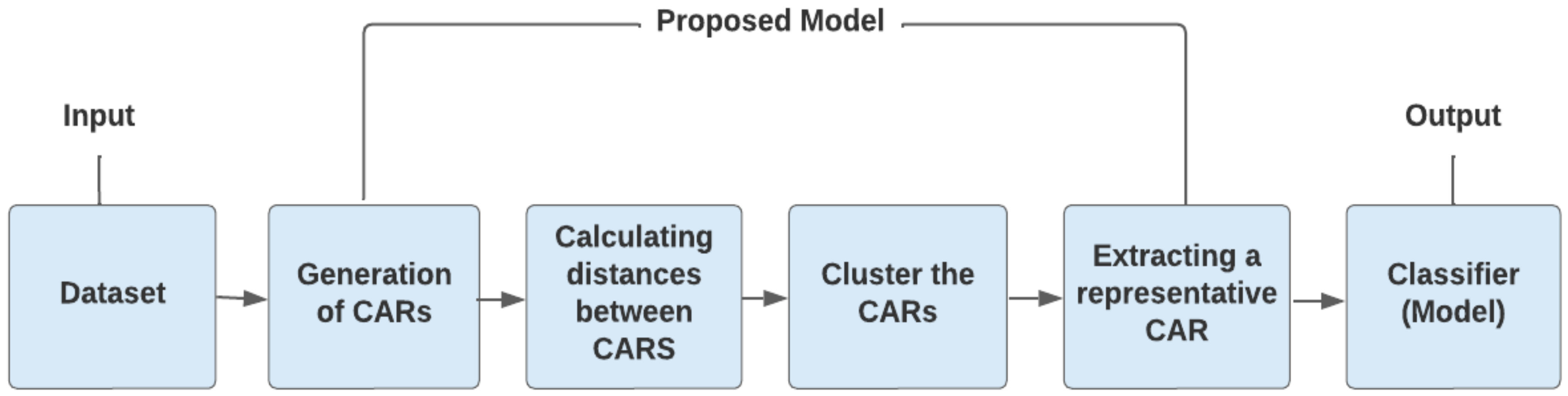
The proposed approach is illustrated in Figure 1. First, the strong CARs in the dataset were mined. Then, novel distance metrics to utilize in the hierarchical clustering algorithm were developed. The final association classifier was formed by extracting a representative CAR for each cluster. Clustering aims to group similar rules together; taking a representative CAR within a cluster eliminates the rule-overlapping issue while reducing the classifier’s size.

Each of the steps mentioned in the above figure is described in the following subsections.

3.1. Class Association Rules

This subsection focuses on finding “interesting” associations between attributes and class labels in the dataset: the generation of strong CARs. The generation of ARs (CARs) is expressed in two steps: (1) finding the frequent itemsets (the itemsets that satisfy the user-specified conditions) in the dataset and (2) association rule generation from frequent itemsets. While the second step is straightforward, the first step is extremely crucial in the construction of strong CARs. Before generating the CARs, we describe the basic rule evaluation metrics, which we use later. Rule-evaluation metrics for the rule $\left\{A\Rightarrow B\right\}$ are expressed below:

$$supp \left(A\Rightarrow B\right)=supp \left(A\cup B\right)=\frac{supp\_count \left(A⟹B\right)}{T}$$

(1)

where $supp\_count \left(A⟹B\right)$ is the number of records that include both A and B. T is the total number of records.

Confidence of the rule is a percentage value that shows how often each item in B appears in records that contain items in A. It computes the strength of the rule, that is, the correlation between antecedent and consequent.

$$conf \left(A\Rightarrow B\right)=\frac{supp \left(A\cup B\right)}{supp \left(A\right)}$$

(2)

The lift of the rule is computed by dividing the confidence by the expected confidence. The expected confidence is the support of the consequences of the rule.

$$lift \left(A\Rightarrow B\right)=\frac{conf \left(A\Rightarrow B\right)}{supp \left(B\right)}$$

(3)

A dynamic algorithm called “APRIORI” is utilized to generate the class association rules. APRIORI is significantly more time-efficient compared to other frequently used mining algorithms, easy to implement, and sound enough to make fair comparisons with other AC methods. APRIORI uses a bottom-up approach that generates a 1-frequent itemset (includes one item only), whose support is greater than the user-specified threshold in the initial stage. In the next step, the 2-frequent itemset is found based on the 1-frequent itemset, and this procedure lasts to produce all the frequent itemsets. The APRIORI algorithm was simplified in our case because we generated the frequent itemsets containing class attributes.

Class association rules are generated from frequent itemsets found by APRIORI, which satisfy a user-defined minimum confidence threshold. Since the APRIORI generates frequent itemsets containing class attributes, the CAR-generation step is straightforward. For each itemset F containing Class C, all nonempty subsets of F are generated, and then every nonempty subset S of F, strong CAR R, is outputted in the form of “S→C” if, $Confidence \left(R\right)\ge min\_conf$, where min_conf is the minimum confidence threshold.

3.2. Similarity Measures

In this section, the significant impact of similarity measures (also called distance metrics) used to produce an accurate and compact model is demonstrated. Since there is a lack of distance metrics for CARs, developing such metrics will be an extremely important contribution to the field. After the strong association rules have been generated, as described in Section 3.1, they are then clustered. Since hierarchical agglomerative clustering will be used, the similarity (how far apart the two rules are) between CARs needs to be measured. Research studies have suggested a few indirect distance metrics for association rules, such as Absolute Market-Basket Difference (AMBD) [39], Conditional Market-Basket Probability (CMBP) and Conditional Market-Basket Log-Likelihood (CMBL) [40], as well as Tightness [41].

3.2.1. Indirect and Direct Distance Metrics

Rule distances that are obtained from data are called Indirect Distance Metrics, which are defined as a function of the market-basket sets that support two considered rules.

For the purpose of clustering association rules, Natarajan and Shekar introduced a measure called “tightness”, which emphasizes the strength of the correlation between the items of an association rule. The premise of this technique is that correlated items tend to occur together in transactions. “Tightness” is different from traditional support or confidence measures. More precisely, the support values for the most and least frequent items of an association rule were considered for computing the distance.

Let $x_1{x}_2\dots x_m\to \cdots \dots x_n$ be an association rule and the $\dots =1\dots n$ its respective items. $S_{x_i}$ denotes the support of item $x_i$. Support values for the most and least frequent items of association rule r are given by $S_{r_{\max }}=\max \left(S_{\dots },\dots ,S_{x_n}\right)$ and $S_{r_{\min }}=\min \left(\dots ,\dots ,S_{x_n}\right)$. The tightness measure is defined as follows:

$$T=\frac{S_r}{\left(\frac{S_{r_{\max }}+S_{r_{\min }}}{2}\right)-S_r}$$

T reaches its maximum (i.e., ∞) when $S_{r_{\max }}+S_{r_{\min }}=S_r$. Based on the notion of tightness, the following distance measure has been introduced:

$$d\left(r_1,r_2\right)=\frac{\left|T_{r_1}-T_{r_2}\right|}{T_{r_1}+T_{r_2}}$$

As Natarajan and Shekar have shown in the context of market basket analysis, this measure is able to discover similar purchasing behaviors in different item domains and is appropriate for association rules.

In connection with association rule mining, ref. [39] presented their approach to mitigating the rule quantity problem with pruning and grouping techniques. They proposed clustering the rules by introducing the following simple distance measure based on database coverage between association rules with the same consequence. The distance $d^{AMBD}$ between rule1 and rule2 is the (estimated) probability that one rule does not hold for a basket, given that at least one rule holds for the same basket. Based on the number of non-overlapping market baskets, a distance metric can be defined as follows:

$$d_{rule1,rule2}^{AMBD}=m\left(B{S}_{rule1}\right)+m\left(B{S}_{rule2}\right)-2\ast \left|m\left(B{S}_{rule1},B{S}_{rule2}\right)\right|$$

(4)

where BS is both sides of the rule; that is, the itemset for the association rule. m(BS) denotes the support of a rule. In Equation (4), rules with similar tuples obtain a lower distance than the rules with dissimilar tuples. More specifically, the distance indicates the percentage of tuples in the dataset that are not covered by either rule. This approach, while intuitive and applicable only for rules with the same consequent, is appropriate for measuring the similarity of class association rules.

Since the rules are clustered by class label, the distance is computed by ignoring the class label. When applying indirect distance metrics to our proposed method, a larger number of clusters is found, meaning the classifiers included a large number of rules. This issue was a research motivation to propose a new normalized distance metric based on “direct” measures, called Item Based Distance Measure (IBDM), in this research paper by considering the differences in rule items.

Let $R: \left\{a_1,a_2,\dots .,a_n\right\}\Rightarrow C$ be a class association rule where, $a_{i, }\left(i=1\dots n\right)$ is rule items (attributes’ values), n is the total number of attributes (the number of rule items cannot exceed n), and C is a class label. Given two rules $rule1: \left\{a_1,a_2,\dots .,a_m\right\}\Rightarrow C, rule2: \left\{a_1,a_2,\dots .,a_k\right\}\Rightarrow C. rule1, rule2\in R$ and 1 ≤ m, k ≤ n, we compute the similarity as follows:

$$similarity\left(index\right)=\left\{\begin{array}{c} if (a_{index}^{rule1}=a_{index}^{rule2}) | (a_{index}^{rule1}=\varnothing and a_{index}^{rule2}=\varnothing ), 0;\\ else if (a_{index}^{rule1}=\varnothing and a_{index}^{rule2}\ne \varnothing ) | (a_{index}^{rule1}\ne \varnothing and a_{index}^{rule2}=\varnothing ) , 1; \\ else 2 \left(a_{index}^{rule1}\ne a_{index}^{rule2}\right).\end{array}\right.$$

(5)

where index is the index of rule items. The similarity function (5) has a low value when the rules have similar items. A rule item that is empty is regarded as being closer than one that is different. The distance between the two rules is denoted as follows:

$$d_{rule1,rule2}^{IBDM}={\sum }_{i=1}^{n}similarit{y}_i/(2\times n)$$

(6)

The range of distance (6) is between 0 and 1. The distance between CARs that contain the same things is 0, while the distance between CARs that contain different items is 1.

3.2.2. The New “Weighted and Combined” Distance Metrics

The AMBD metric is appropriate for measuring the similarity of rules with the same consequence, and IBDM is also proposed for that purpose (to compute the similarity of CARs). Aiming at applying these distance metrics to cluster the CARs with the same class, an efficient distance metric, Weighted and Combined Distance Metric (WCDM), is developed by merging the IBDM and AMBD distance metrics. The advantage of WCDM is that it considers the direct measure (rule items) and the indirect measure (rule coverage). The $d^{\mathrm{WCDM}}$ between two rules, rule1 and rule2, is defined below:

$$d_{rule1,rule2}^{WCDM}=\alpha \times d_{rule1,rule2}^{IBDM}+\left(1-\alpha \right)\times d_{rule1,rule2}^{AMBD}$$

(7)

where $\alpha \mathrm{is} \mathrm{weight} \mathrm{parameter}$, $d^{IBSM}$ is a direct distance metric and $d^{AMBD}$ is an indirect distance metric.

When we apply AMBD ($\alpha =0$) distance metric in the proposed method, a larger average number of clusters with slightly better accuracy is obtained. When the IBDM ($\alpha =1$) was applied, the distance metric to the proposed method showed a smaller average number of clusters with slightly lower accuracy. After performing some experiments, different $\alpha$ parameters were determined to show how the distance metrics affected the performance of the classifier. The following distance metrics are developed:

Weighted Combined and Balanced (WCB): The $\alpha =0.5$ parameter was set in the distance metric developing part; that is, the contribution of IBDM and AMBD was considered equal to make the balanced distance metric. The resulting distance metric is defined in Equation (8).

$$d_{rule1,rule2}^{WCB}=0.5\times d_{rule1,rule2}^{IBDM}+0.5\times d_{rule1,rule2}^{AMBD}.$$

(8)

Weighted Combined and Indirect advantage (WCI): The α = 0.25 parameter was set in the distance metric developing part; the majority part of the “Combined” distance metric becomes the “Indirect” distance metric that is shown in Equation (9).

$$d_{rule1,rule2}^{WCI}=0.25\times d_{rule1,rule2}^{IBDM}+0.75\times d_{rule1,rule2}^{AMBD}.$$

(9)

Weighted Combined and Direct Advantage (WCD): The $\alpha =0.75$ parameter was set in the distance metric developing part, and the majority of the “Combined” distance metric became the “Direct” distance metric that is expressed in Equation (10).

$$d_{rule1,rule2}^{WCD}=0.75\times d_{rule1,rule2}^{IBDM}+0.25\times d_{rule1,rule2}^{AMBD}.$$

(10)

3.3. Clustering of Class Association Rules

The goal of clustering rules is to group related rules; rules in one cluster should be related to and distinct from rules in other clusters.

Hierarchical clustering techniques come in two types: top-down (divisive hierarchical clustering) and bottom-up (hierarchical agglomerative clustering). In the beginning, bottom-up algorithms treat each example as a separate cluster. However, after each iteration, they combined the two closest clusters into a single cluster that comprised all the examples. A tree (or dendrogram) is used to illustrate the cluster structure that results. In contrast to the hierarchical agglomerative clustering method, the top–down strategy. It considers every case in a single cluster before breaking it up into smaller pieces until every example forms a cluster or meets the stopping condition.

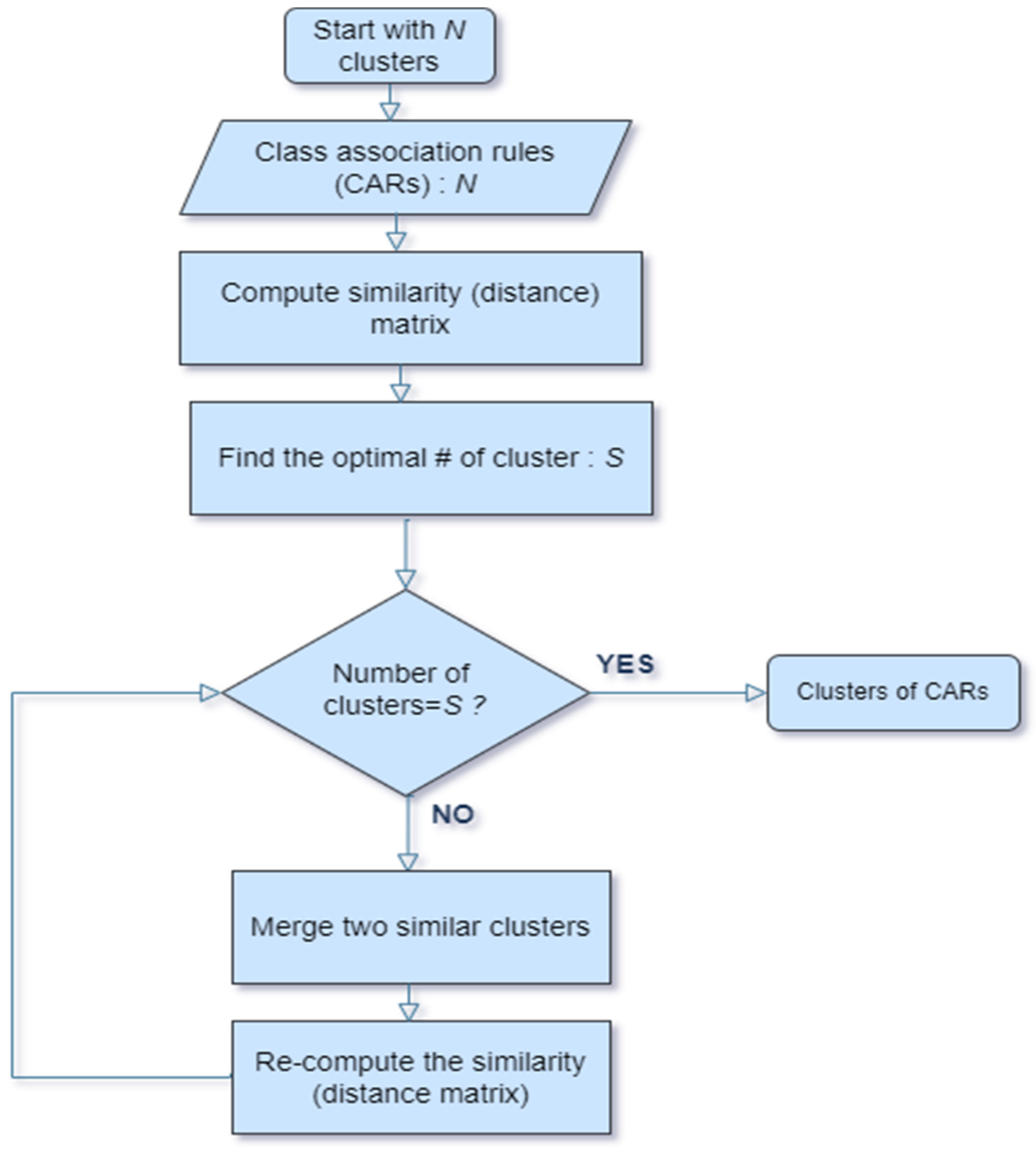
We applied the complete linkage method of hierarchical agglomerative clustering. In the complete linkage (farthest neighbor) method, the similarity of two clusters is the similarity of their most dissimilar examples; therefore, the distance between the farthest groups is taken as an intra-cluster distance. Figure 2 illustrates the clustering phase of the developed algorithm in which each rule is first regarded as a separate cluster (let us assume N CARs are generated). Utilizing the distance measures outlined in Section 3.2.2, a similarity (distance) matrix is built. The hierarchical clustering process needs to be used twice: first, to determine the cluster heights, which will be used subsequently to determine the ideal number of clusters. The “natural” number of clusters is found when the dendrogram is “cut” at the point that represents the maximum distance between two consecutive clusters merging. Agglomerative hierarchical clustering is once more used to identify the clusters of class association rules after the ideal number of clusters has been determined.

3.4. Extracting the Representative CAR

The representative CAR for each cluster must be extracted once we have identified all clusters to create a descriptive, compact, and useful associative classifier. In this procedure, the CAR closest to the cluster’s center is selected as a representative; hence, the representative CAR must have the minimum average distance from all other rules. The method is described in Algorithm 1.

Algorithm 1 A representative car based on cluster center (rc)
	Input: a set of class association rules (CAR) in CARs array
	Output: A representative class association rule
1	Initialization: assign length of CARs array to N, maximum value of Float to min_distance, zero to i and j
2	while (i < N) do// Read all the CARs in CARs array
3	assign zero to distance and j
4		while (j < N) do// Find the average distance between CAR i and all other CARs
5			distance  $\leftarrow$ distance  $+$  compute the similarity between rule i and rule j  by using WCB | WCI | WCD distance metrics
6			jump to next rule, increase the value of j by 1
7		End
8		average_distance$\leftarrow$distance / N
9		if (avg_distance < min_ distance) then
10			assign avg_distance to min_distance
11			assign CAR i to representative_CAR
12		Endif
13		jump to next rule, increase the value of i by 1
14	End
15	return representative_CAR

Algorithm 1 gets a set of CARs within a cluster as an input. Lines 4–7 calculate the distance from the chosen CAR to all the other CARs using the distance variable (one of the distance measures described in Section 3.2.2 is used). In line 10, the starting value of min_distance is the maximum value of the float and is used to store the minimum average distance. In lines 9–12, the representative CAR that has the lowest average distance from all the other rules is identified. Algorithm 2 demonstrates our proposed approach step-by-step below:

Algorithm 2 Developed Associative Classification Model
	Input: A dataset D, minimum support and minimum confidence
	Output: A compact and accurate model
1	Initialization of variables: assign the number of classes to N, zero to i and j
2	Generate the class association rules (CAR) by applying the APRIORI algorithm
3	Group the CARs based on class label
4	while (i < N) do //We do cluster for each group (class) of CARs
5		compute the similarity matrix of CARs belonging to group i by using one of the distance metrics: WCB | WCI | WCD
6		do cluster to obtain the cluster_heights // HCCL algorithm is used to cluster the CARs
7		Find the optimal number of clusters C by using cluster_heights
8		perform clustering to identify the clusters of CARs // HCCL algorithm is employed with defined parameter (number of cluster) C
9		assign zero to j
10		while (j < C) do // A representative CAR is extracted for each cluster
11			extract a representative CAR among CARs in cluster j // RC method is utilized to extract a representative CAR defined in Algorithm 1
12			add representative CAR to the model
13			jump to next cluster, increase the value of j by 1
14		End
15		jump to next class, increase the value of i by 1
16	End
17	return model

Algorithm 2 describes every step of the proposed model. The model is given a dataset with minimum support and confidence constraints, which are used to produce class association rules. CARs are organized into groups based on their class labels in line 3. For each group of CARs (lines 4–14), the hierarchical clustering algorithm complete linkage method (HCCL) builds the distance matrix using one of the distance measures described in Section 3.2.2 (line 5), computes the cluster heights (distances between clusters) using the distance matrix in line 6, and then uses these heights (distances) to calculate the ideal number of clusters (line 7). Then, to locate the clusters of CARs, the HCCL method is employed once again. Lines 10–14 extract the representative CAR for each cluster using the technique outlined in Section 3.4 and then incorporate it into our final classifier.

The following classifiers were constructed: CCC1 was built based on WCB; CCC2 was formed based on WCI; CCC3 was formed based on WCD; and all algorithms used the RC method defined in Algorithm 1 for extracting a representative CAR (based on cluster center).

4. Experimental Evaluation

Empirical evaluations were performed on 12 real-life datasets taken from the UCI ML Repository. The developed associative classifiers were compared with 6 associative classifiers (CBA and our previously developed classifiers: SA, J&B, DC, DDC, and CDC) on accuracy and size. We also included the Majority Class Classifier (MCC) in the comparison to see if AC algorithms have problems classifying minority classes. The new associative classifiers were compared with the above-mentioned AC methods because in previous research [28,29,31], a comprehensive evaluation of our above-mentioned AC methods with well-known rule-based classification models was already provided. This study utilized a paired t-test (with a 95% significance threshold) method of statistical significance testing to present the statistical differences in the obtained results. A paired t-test is used to compare the means of two sample sets when each observation in one sample could be paired with an observation in the other sample. In our case, two sample sets are the classification accuracies of two models over a 10-fold cross-validation method (10 pairs of results, a pair of results for each fold).

The same default parameters were applied for all AC methods; to make a fair comparison, min_support, and min_confidence thresholds were set to 1% and 60%, respectively, as default parameters. In some datasets, minimum support was lowered to 0.5% or even 0.1%, and confidence was lowered to 50% to ensure “enough” CARs (“enough” means at least 5–10 rules for each class value; this situation mainly happens with imbalanced datasets) were generated for each class value. We utilized the WEKA workbench [42] implementation of all associative classifiers.

A 10-fold cross-validation evaluation protocol was used to perform the experiments. The descriptions of the datasets and input parameters of the AC methods are shown in

Table 1. Description of datasets and AC algorithm parameters.

Dataset	# of Attributes	# of Classes	Class Distribution	# of Records	Min Support	Min Confidence	# of Analyzed Rules
Breast.Can	10	2	201; 85	286	1%	60%	1000
Balance	5	3	288; 49; 288	625	1%	50%	218
Car.Evn	7	4	1210; 384; 69; 65	1728	1%	50%	1000
Vote	17	2	267; 168	435	1%	60%	500
Tic-Tac	10	2	626; 332	958	1%	60%	3000
Nursery	9	5	4320; 2; 328; 4266; 4044	12,960	0.5%	50%	3000
Hayes.R	6	3	65; 64; 31	160	0.1%	50%	1000
Lymp	19	4	2; 81; 61; 4	148	1%	60%	1500
Spect.H	23	2	56; 211	267	0.5%	50%	3000
Adult	15	2	34,013; 11,208	45,221	0.5%	60%	5000
Chess	37	2	2839; 357	3196	0.5%	60%	3000
Connect4	43	3	44,473; 16,635; 6449	67,557	1%	60%	5000

.

Table 2. Overall accuracies with standard deviations.

Dataset	MCC	CBA	SA	J&B	DC	DDC	CDC	CCC1	CCC2	CCC3
Breast.Can	70.2	$71.9 \pm 9.8$	$79.3 \pm 4.4$	$80.5 \pm 4.7$	$81.2 \pm 4.0$	$81.9 \pm 4.1$	$\mathbf{82.6}\mathbf{ }\mathbf{\pm }\mathbf{ }\mathbf{4.5}$	$80.9 \pm 5.1$	$81.2 \pm 4.9$	$80.8 \pm 4.8$
Balance	46.1	$73.2 \pm 3.8$	$74.0 \pm 4.1$	$74.1 \pm 2.6$	$72.8 \pm 2.4$	$73.2 \pm 2.9$	$73.2 \pm 3.0$	$\mathbf{75.9}\mathbf{ }\mathbf{\pm }\mathbf{ }\mathbf{2.1}$	$74.7 \pm 2.4$	$74.1 \pm 2.7$
Car.Evn	70.0	$\mathbf{91.2}\mathbf{ }\mathbf{\pm }\mathbf{ }\mathbf{3.9}$	$86.2 \pm 2.1$	$89.4 \pm 1.4$	$85.8 \pm 1.4$	$88.9 \pm 1.2$	$87.1 \pm 1.6$	$87.5 \pm 1.9$	$88.9 \pm 1.6$	$88.1 \pm 1.8$
Vote	61.4	$94.4 \pm 2.6$	$\mathbf{94.7}\mathbf{ }\mathbf{\pm }\mathbf{ }\mathbf{2.3}$	$94.1 \pm 1.8$	$92.9 \pm 2.5$	$93.2 \pm 2.8$	$90.6 \pm 2.3$	$91.8 \pm 1.9$	$91.6 \pm 2.3$	$92.5 \pm 2.0$
Tic-Tac	65.3	$\mathbf{100.0}\mathbf{ }\mathbf{\pm }\mathbf{ }\mathbf{0.0}$	$91.7 \pm 1.5$	$95.8 \pm 2.0$	$87.3 \pm 1.3$	$91.8 \pm 1.0$	$92.4 \pm 1.1$	$89.0 \pm 1.4$	$88.1 \pm 1.2$	$89.7 \pm 1.5$
Nursery	33.3	$92.1 \pm 2.4$	$91.6 \pm 1.2$	$89.6 \pm 1.1$	$88.5 \pm 1.1$	$89.3 \pm 1.1$	$92.3 \pm 0.9$	$90.4 \pm 0.7$	$\mathbf{92.9}\mathbf{ }\mathbf{\pm }\mathbf{ }\mathbf{0.8}$	$88.1 \pm 0.7$
Hayes.R	40.6	$75.6 \pm 10.9$	$73.1 \pm 6.0$	$79.3 \pm 5.9$	$79.9 \pm 5.7$	$77.8 \pm 5.2$	$\mathbf{82.7}\mathbf{ }\mathbf{\pm }\mathbf{ }\mathbf{6.1}$	$81.0 \pm 6.0$	$81.4 \pm 6.5$	$78.1 \pm 6.9$
Lymp	54.7	$79.0 \pm 9.7$	$73.7 \pm 5.1$	$80.6 \pm 5.7$	$78.4 \pm 6.7$	$80.0 \pm 6.1$	$\mathbf{84.0}\mathbf{ }\mathbf{\pm }\mathbf{ }\mathbf{6.4}$	$80.2 \pm 7.1$	$79.7 \pm 6.4$	$79.2 \pm 6.7$
Spect.H	79.0	$79.0 \pm 1.6$	$79.1 \pm 2.1$	$79.7 \pm 3.1$	$81.5 \pm 0.7$	$81.3 \pm 1.1$	$\mathbf{82.8}\mathbf{ }\mathbf{\pm }\mathbf{ }\mathbf{1.3}$	$80.6 \pm 1.1$	$80.8 \pm 1.0$	$80.0 \pm 1.0$
Adult	75.2	$81.8 \pm 3.4$	$80.8 \pm 2.6$	$80.8 \pm 2.9$	$81.9 \pm 2.4$	$82.0 \pm 2.6$	$\mathbf{82.8}\mathbf{ }\mathbf{\pm }\mathbf{ }\mathbf{3.0}$	$81.3 \pm 2.4$	$81.4 \pm 2.8$	$81.8 \pm 3.2$
Chess	88.8	$95.4 \pm 2.9$	$92.2 \pm 3.8$	$94.6 \pm 2.7$	$97.0 \pm 2.0$	$97.3 \pm 2.0$	$\mathbf{97.8}\mathbf{ }\mathbf{\pm }\mathbf{ }\mathbf{2.0}$	$97.1 \pm 1.6$	$96.8 \pm 1.6$	$96.1 \pm 1.9$
Connect4	65.8	$80.9 \pm 8.1$	$78.7 \pm 6.0$	$81.0 \pm 5.2$	$80.0 \pm 5.9$	$80.7 \pm 5.9$	$\mathbf{81.7}\mathbf{ }\mathbf{\pm }\mathbf{ }\mathbf{5.9}$	$81.2 \pm 6.9$	$\mathbf{81.7}\mathbf{ }\mathbf{\pm }\mathbf{ }\mathbf{6.6}$	$81.0 \pm 6.0$
Average (%):	62.5	$84.5 \pm 4.9$	$82.3 \pm 3.4$	$84.9 \pm 3.3$	$83.9 \pm 3.0$	$84.7 \pm 3.0$	$85.8 \pm 3.2$	$84.7 \pm 3.2$	$84.9 \pm 3.1$	$84.1 \pm 3.3$

Bold result means the best accuracy for each dataset

illustrates the experimental results on classification accuracies (average values over the 10-fold cross-validation with standard deviations). The best accuracy for each dataset was shown in bold.

Overall observations on accuracy (shown in Table 2) reveal that newly developed techniques CCC1, CCC2, and CCC3 achieved an average accuracy that was comparable to the other associative classifiers (84.7%, 84.9%, and 84.1% respectively). The average accuracy of CCC2 was higher than the CCC1 and CCC3 approaches (and higher than CBA, SA, DC, and DDC as well), while the J&B and CDC algorithms produced results that were similar or slightly higher. Noticeably, the proposed methods achieved the best accuracy on the “Balance” (CC1: 75.9%), “Nursery” (CCC2: 92.9%), and “Connect4” (CCC2: 81.7%) datasets among all AC methods. The developed classifiers received lower results on the “Tic-Tac” dataset than the other algorithms (except DC).

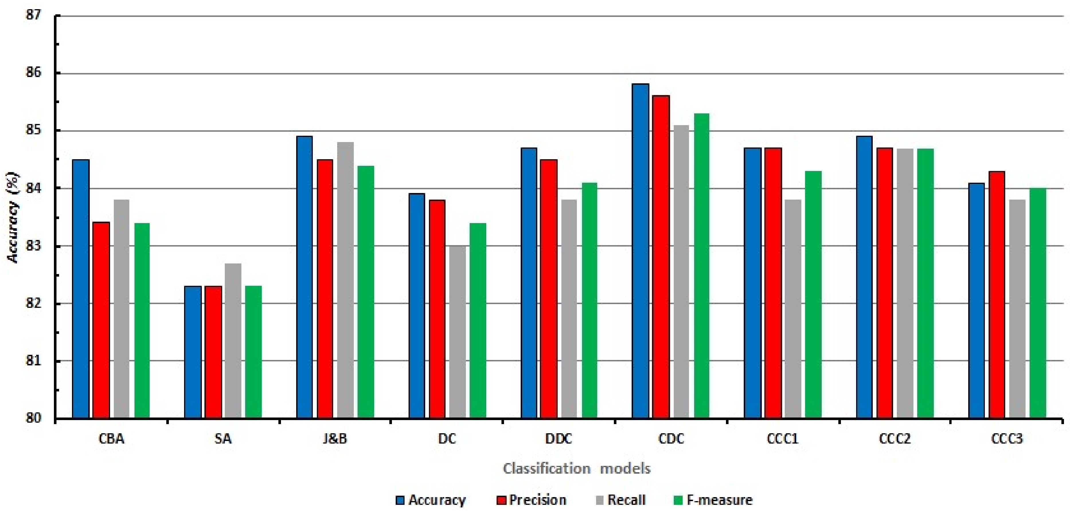
Figure 3 shows the comparison of the overall performance of the classifiers on average accuracy and other evaluation metrics such as “Precision,” “Recall,” and “F-measure” to see how reliable the achieved accuracies by associative classification models. Weighted (based on class distribution) average results of the Precision, Recall, and F-measure were reported, and the detailed information on evaluation metrics for each dataset is provided in Appendix A.

The statistical differences were measured (wins/losses counts) on accuracy between CCC1, CCC2, CCC3, and other AC models (shown in

Table 3. Statistically significant wins/losses counts of CCC1 method on accuracy.

	CBA	SA	J&B	DC	DDC	CDC	CCC2	CCC3
W	3	4	1	1	2	1	0	2
L	3	2	2	0	1	3	1	0
N	6	6	9	11	9	8	11	10

). W: our approach was significantly better than the compared algorithm; L: selected rule-learning algorithm significantly outperformed our algorithm; N: no significant difference has been detected in the comparison.

Table 3 shows that CCC1 obtained the comparable results with AC methods included in the comparison. However, CCC1 lost to J&B. CDC and CCC2 methods according to win/losses counts (CCC1 has more losses than wins compared to those algorithms); there was no statistical difference between them on the 8, 9, and 11 datasets out of 12. The same experiment was carried out for CCC2, as shown in

Table 4. Statistically significant wins/losses counts of CCC2 method on accuracy.

	CBA	SA	J&B	DC	DDC	CDC	CCC3
W	2	5	3	2	2	0	2
L	3	2	2	0	1	3	0
N	7	5	7	10	9	9	10

.

Interestingly, CCC2 did not get worse accuracy than DC and CCC3 methods on any datasets. Even though CCC2 lost to the CBA and CDC algorithms, it won the rest of the algorithms in accuracy due to wins/losses counts.

Table 5. Statistically significant wins/losses counts of CCC3 method on accuracy.

	CBA	SA	J&B	DC	DDC	CDC
W	2	3	0	2	0	1
L	3	3	1	0	1	5
N	7	6	11	10	11	6

defines the wins/losses counts of the CCC3 method. The results showed that the CCC3 method obtained a slightly lower result than all other AC methods in terms of statistical win/loss counts except for DC and SA. However, on average, the classification accuracies of CCC3 are not much different from those of the other 8 associative classifiers.

Experimental evaluations of the number of rules generated by classifiers are shown in

Table 6. Number of CARs.

Dataset	CBA	SA	J&B	DC&DDC	CDC&CCC1	CCC2	CCC3
Breast.Can	63	20	47	8	9	11	9
Balance	77	45	79	34	79	86	61
Car.Evn	72	160	41	32	32	37	32
Vote	22	30	13	6	6	6	9
Tic-Tac	23	60	14	24	17	27	21
Nursery	141	175	109	79	80	114	74
Hayes.R	34	45	34	19	80	80	37
Lymp	23	60	29	5	7	6	5
Spect.H	4	50	11	8	5	7	6
Adult	126	130	97	13	88	101	79
Chess	12	120	24	12	17	14	14
Connect4	349	600	273	59	102	146	117
Average:	79	125	64	25	43	53	39

(The best result for each dataset was bolded). Since the size of DC, DDC (DC and DDC utilized the same “direct” distance metric for clustering, further producing the same number of rules), and CDC, CCC1 (CDC and CCC1 methods employed the same “indirect” distance metric for clustering) are the same, these algorithms are merged in the resulting table.

Table 6 shows that the proposed methods achieved the second-highest result on the average number of rules, the only classifier that performed better was the DC classifier. Surprisingly, the developed methods produced unexpectedly large classifiers on the “Balance” and “Hayes.R” datasets. Overall, CCC1, CCC2, and CCC3 produced classifiers similar to other AC methods included in the study on size.

An interesting and expected fact is that if we increase the $\alpha$ parameter (that means that the majority of the “Combined” distance metric becomes the “Indirect” distance metric), we get the higher average number of rules with slightly better average accuracy. If we decrease the $\alpha$ parameter (that means that the majority of the “Combined” distance metric becomes the “Direct” distance metric), we get the lower average number of rules with slightly worse average accuracy. The statistical significance testing (win/loss counts) results are shown in

Table 7. Statistically significant wins/losses counts of CCC1 method on number of rules.

	CBA	SA	J&B	DC&DDC	CCC2	CCC3
W	8	10	9	2	6	3
L	2	2	2	5	1	5
N	2	0	1	5	5	4

,

Table 8. Statistically significant wins/losses counts of CCC2 method on the number of rules.

	CBA	SA	J&B	DC&DDC	CCC3
W	7	10	7	0	1
L	4	2	5	7	7
N	1	0	0	5	4

and

Table 9. Statistically significant wins/losses counts of CCC3 method on the number of rules.

	CBA	SA	J&B	DC&DDC
W	8	11	10	2
L	1	1	2	5
N	3	0	0	5

for each proposed classifier. Statistically significant counts (wins/losses) of CCC1 against other rule-based classification models on classification rules are shown in Table 7.

In terms of number of rules, our suggested classifiers provided results comparable to cluster-based AC methods (DC, DDC, CCC3), but these results were better than those of other AC algorithms (CBA, SA, J&B). On the importance of win/loss counts, CCC1 produced significantly smaller classifiers than CBA, SA, J&B, and CCC2 on more than half of the datasets but did not perform as well as DC, DDC, and CCC3 algorithms (it generated the larger classifier on 5 out of the 12 datasets).

The CCC2 classifier performed the worst among the newly developed methods (CCC1, CCC3) on size. Although CCC2 produced larger classifiers than DC, DDC, and CCC3 on 7 datasets out of 12, it achieved a better result than CBA, SA, and J&B methods according to significant wins/losses counts.

Table 9 represents that CCC3 outperformed all AC methods except DC and DDC in terms of classification rules. It generated a larger classifier on only 1 dataset than CBA, SA, and 2 datasets out of 12 than J&B.

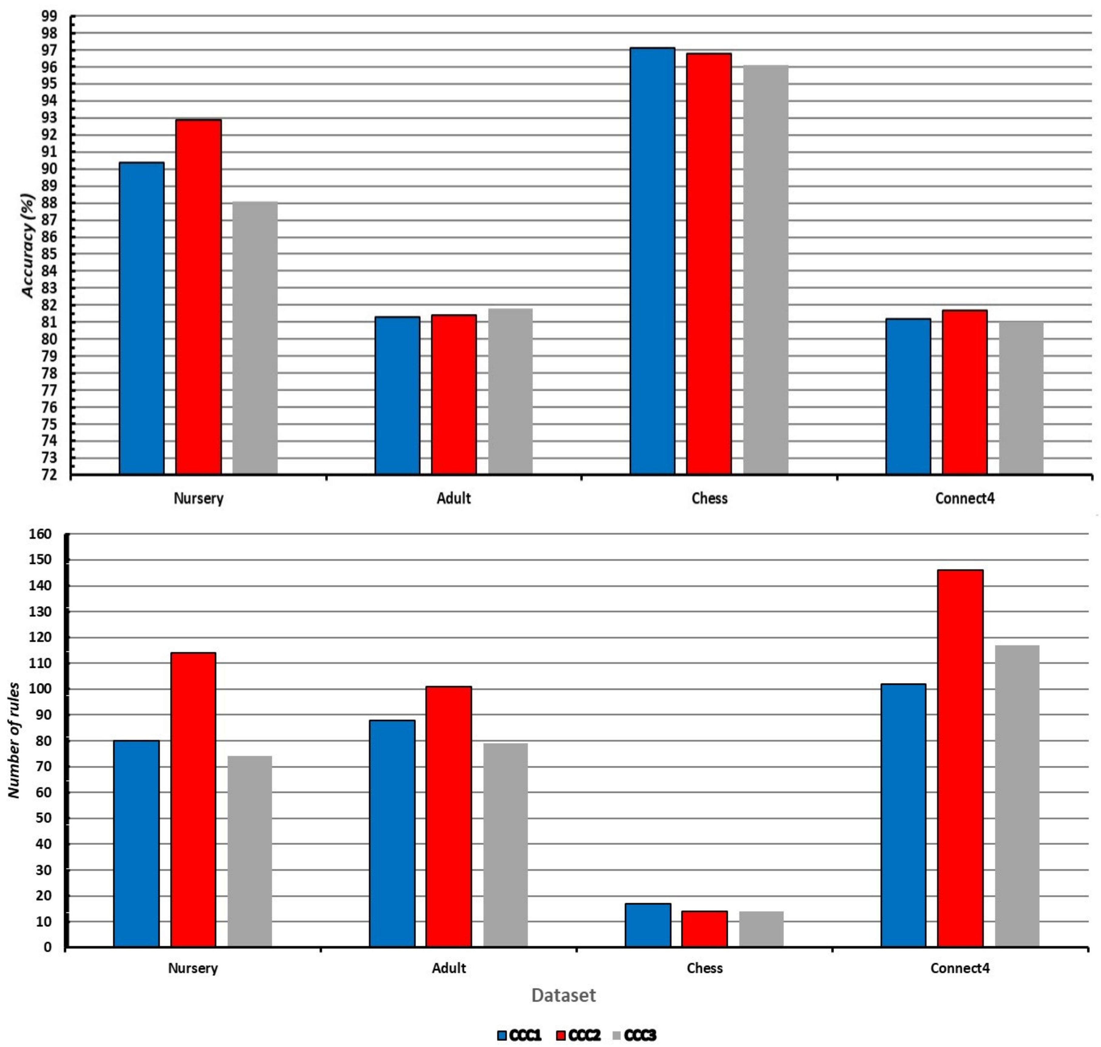
We analyzed the performance (on accuracy and rules) of the developed methods on “bigger” datasets, as shown in Figure 4. Since our main goal is to produce compact models and show the influence of distance metrics (importance of α parameter) for developing such models, we analyzed the performance of the newly developed models on bigger datasets.

Figure 3 illustrates that the accuracies of CCC1, CCC2, and CCC3 classifiers were almost the same as each other on the selected bigger datasets. Regarding accuracy, CCC2 achieved a slightly better result than CCC1 and CCC3, while it obtained a worse result than those methods in terms of classification rules (shown in Figure 4), which is expected behavior.

5. Discussion

The DC, DDC, and CDC cluster-based associative classification algorithms are similar to our developed methods. All algorithms utilize the “APRIORI” algorithm to generate the strong class association rules and hierarchical clustering algorithm to cluster the CARs. After clustering the CARs, the representative CAR is selected for each cluster to produce the final classifier. The DC method was built based on a “direct” (depending only on rule items) distance measure (for clustering purposes), and the method for extracting a representative CAR was based on a cluster center. The DDC method was formed based on a “direct” (depending only on rule items) distance measure, and the method for extracting a representative CAR was based on database coverage. The CDC method was formed based on the “combined” (depending only on rule items and database coverage) distance measure, and the method for extracting a representative CAR was based on database coverage. The key differences between the newly developed methods and the DC, DDC, and CDC methods are that the proposed methods applied a “combined” distance metric (with different parameters), and a representative CAR was extracted based on the cluster center.

The newly developed models were comparable to all aforementioned associative classification models, both in accuracy and size. The most important advantage of our proposed methods was to generate a smaller classifier on bigger datasets compared to associative and traditional (a previous study proved that traditional rule-based algorithms are sensitive to dataset size) rule-learners.

We also tried to measure the accuracy and other evaluation measures (Precision, Recall, and F-measure) of the complete rule set without clustering and representative rule extraction, but the accuracies were never better than the best accuracy in the result table.

Our proposed algorithm has some limitations:

• To obtain enough class association rules for each class value, we need to apply appropriate minimum support and minimum confidence thresholds. That is, we should take into consideration the class distribution of each dataset;
• Associative classifiers may get lower results in terms of classification accuracy than other traditional classification methods on imbalanced datasets, because imbalanced class distribution may affect the rule-generation part of associative classification algorithms;
• The newly developed distance metric is dependable to α parameter: if we lower the α parameter, we get a higher number of clusters (higher number of rules) with better accuracy, and if we increase the α parameter, we obtain a smaller classifier with slightly lower accuracy, which is an expected behavior.

6. Conclusions

According to experimental evaluations, the CCC1, CCC2, and CCC3 classifiers could reduce the number of classification rules while still maintaining classification accuracy that was on par with other AC approaches included in the comparison. Compared to cutting-edge classification models, it created classifiers that were significantly smaller.

Each of the three associative classifiers that have been built has a different advantage on specific datasets, and they are even competitive in terms of classification accuracy and the number of rules produced.

Another promising direction for future research on associative classifiers is to investigate ways of including numeric attributes in the models. There is already ongoing research in this area, but using clustering on CARs may open new potentially interesting perspectives on the matter.