Modeling of Water Losses in Hydraulic Tunnels under Pressure Based on Stepwise Regression Method

Abstract

In this paper, we presented a methodology for efficient and accurate modeling of water losses in hydraulic tunnels under inside internal water pressure, based on multiple linear regression (MLR). The methodology encompasses all steps needed to obtain an adequate mathematical relation between total water losses and relevant measurements in the tunnel, such as reservoir water level, piezometric levels, concrete and water temperatures, size of cracks, etc. Once the data are preprocessed and input variables were chosen, correlation analysis and PCA (principal component analysis) reduction were performed in order to obtain the pool of regression functions. Through an iterative process, according to stepwise regression principles, the most adequate MLR model in terms of accuracy and complexity was chosen. The methodology presented has been validated in modeling water losses in the hydraulic tunnel under the pressure of PSHPP “Bajina Bašta” in the Republic of Serbia. The obtained results have shown significantly better accuracy compared to the results published by other authors, proving that the developed model can be used as a powerful tool in future analyses of tunnel losses and remediation planning.

1. Introduction

Hydraulic tunnels subject to the high internal pressure of water (HT) are mostly used to carry water from the reservoir to the hydropower plant machine building with turbines. The hydraulic fall that exists between the reservoir and the power plant produces the internal water pressure in the hydraulic tunnel. Internal water pressure can cause tensile stresses and cracks in concrete tunnel lining and thus generate static instability in terms of failure and functional instability in terms of water losses from the tunnel. The water loss in the tunnel occurs through various cracks and fissures in the concrete lining. Some cracks are clearly visible, while some smaller cracks are not. On the other hand, the rock mass affects the increase or decrease of total water loss, depending on the porosity and degree of jointing of the rock mass. It is because of this that hydrotechnical tunnels are grouted, so as to fill the cracks around the tunnel and therefore lower the permeability of the rock mass. The water lost from inside the tunnel ends up in the surrounding rock mass, which can have an additional negative impact on the mechanical and deformation properties of the rock mass [1,2,3]. Besides the grouting measures for filling the rock mass cracks, the elimination of tensile stresses in the concrete lining, and therefore securing functionality and stability of hydraulic tunnels under pressure, is most effectively achieved by stress injection [4]. Other approaches exist as well, such as the use of reinforced concrete tunnel linings in order to prevent the formation of cracks [5].

In HT, appropriate monitoring is carried out during the structure’s lifetime. Based on the monitoring, appropriate stability and functionality estimates (SaFE) for the tunnel can be made. The assessment of stability and functionality for the HT is performed based on measurements of significant physical quantities and a variety of physical, mathematical, and other models that describe the processes related to HT. The most frequent measurements are water losses in the tunnel, temperature of concrete, the temperature of water and rock, opening and closing of cracks, groundwater levels, and other relevant indicators. For the purpose of SaFE, two approaches are used. The first approach involves emptying the tunnel and physical inspection, which is occasionally done in the tunnels. However, this approach is expensive, it takes several weeks, and emptying the tunnel can be statically unfavorable for the tunnel structure pre-stressed with injection pressure. The second approach, which is used more often in practice, involves the creation of appropriate analytical, statistical, and numerical models. This approach allows for continuous monitoring and understanding of the structure’s behavior. Large deviations between the model and real measurements can be used to make appropriate SaFE indicators.

To the best of the authors’ knowledge, there are not many articles dealing with problems of HT safety and functionality, in particular with problems of water losses from the tunnel. Andjelkovic et al. [4] dealt with modeling of total water losses from the HT in the pumped-storage hydroelectric power plant (PSHPP) “Bajina Bašta”, located in the Republic of Serbia. The authors established the relationship between water levels in the reservoir, water levels in piezometers, water levels in the surge tank, and water and concrete temperatures as input variables and total water loss from the tunnel as the output variable. Problems related to water loss and loss of other fluids also appear in pressurized pipeline systems that are similar to pressurized hydrotechnical tunnels, from a phenomena point of view. There are several research papers dealing with different detection methods and solutions to intermittent leakage in pressurized pipeline systems (water, gas, fuel, and others) due to cracking [6,7,8,9].

Apart from the above, there are papers that tangentially deal with the analysis of water filtration through the rock mass and the tunnel lining. In [10], analytical solutions based on conformal mapping of complex variable methods are derived for two-dimensional, steady seepage into an underwater circular tunnel. In addition to analytical models, a certain number of numerical models have been developed based on methods such as the finite element method. For example, researchers Radovanović et al. [11] analyzed the stress–strain state of the tunnel excavation and stability of the hydraulic tunnel support using the finite element method, taking into consideration the filtration of groundwater into the tunnel. The use of finite element methods is widely used in geotechnical analyses and tunnel design. However, they have their shortcomings—problems with significant deformations, taking into account the discontinuities and joints in rock masses, implementing rock and soil porosity, etc. Because of that, research conducted by [12] analyzes the application of the particle discrete element method taking into account the porosity. This research presents a significant step forward and enables the analysis of hydrotechnical tunnels from the aspect of evaluating the water loss through the geomaterial. The author Rui Vas Rodrigues [5] researched the monitoring of cracks in tunnels pressurized with 1000 kPa of water pressure, taking into account the interaction between the tunnel structure and the rock mass by using analytical equations for stresses, deformations, and reinforcement quantities.

Recently, analytical, statistical, and numerical models have been enriched with various heuristics from the machine learning domain (ML), creating hybrid models that combine their advantages. Javadi [13] analyzed the loss of compressed air in tunnels during construction in situations where there are high pressures from groundwater. In this paper, neural networks were used for estimating air loss in the tunnel, depending on the geological conditions and tunnel dimensions. In [14], phreatic line detection, which is a major challenge in seepage problems, was accomplished with the use of the natural element method (NEM) and genetic algorithm (GA). Zhang et al. [15] analyzed the uncertainty quantification for the mechanical behavior of fully grouted rockbolts using Monte Carlo simulation and the Bayesian method. The use of ML methods in tunnels is present in the paper [16] where the reliability-based design optimization method for rock tunnel support is analyzed.

Although the application of ML models in modern research is often of few benefits, ML models of studied phenomena are characterized by certain disadvantages. The requirement for a large number of measurements, high computational costs, difficulties in assessing individual predictor importance, the difficulty in deriving prediction intervals, and the difficulty of model interpretability are some of the disadvantages. For these reasons, and due to engineering practicality, in this paper, statistical models in the form of multiple linear regression (MLR) were used to model water loss in HT. Ease of understanding, low computational costs, availability of model adequacy tests, and well-founded analysis of the significance of individual regressors represent only some of the advantages of MLR models.

Although MLR represents a classical modeling technique that has been refined for almost two centuries, the problems of creating appropriate regression models in terms of dimensionality and selecting the number and type of regressors are not completely solved. Generally, there are two approaches to solving such problems. One is statistical, based on principal component analysis (PCA) [17,18], partial correlation, and stepwise regression methods [19,20], and the other is a hybrid approach, based on a combination of statistical and ML techniques [21]. The authors have opted for the first approach, which involves PCA dimensionality reduction and the application of the stepwise method in the building of the MLR model.

In accordance with the above, the aim of the paper was to develop a novel methodology for the mathematical modeling of water losses at HT. In addition, the goal was to validate this methodology by building an MLR model of water losses with greater accuracy and reliability, compared to previously developed models of water losses. The case study was carried out for the hydraulic tunnel at PSHPP “Bajina Bašta”, located on the Drina River, which represents one of the most significant hydropower structures in the Republic of Serbia for the production of electrical energy.

The different approaches based on statistical and numerical methods that were discussed have their advantages and their shortcomings. Numerical methods are extremely demanding and complex, and they require the determination of several parameters. On the other hand, they enable filtration and stress–strain analyses of tunnels including the interaction with the rock mass. Statistical methods are widely used for the monitoring and assessment of various hydrotechnical structures (majorly dams). They are based on MLR techniques, and there are certain issues in defining the type and number of regressors and their dependencies. In the case of new methodologies that are based on the application of PCA and stepwise regression methods, it is possible to define the most influential regressors for the variable that is modeled (total losses). Besides that, compared to other models, the effect of the crack width is taken into account as it has great influence on the total losses, as does the time component.

2. Theoretical Background

Besides data quantity, the number of variables and potential regressors also affects the complexity of the regression model and the required processing time for its generation. It is advised to consider methods of reducing the potential complexity of the model using techniques of factor analysis. For this purpose, we utilized PCA. The principal components (PC) are the basis for further creation of MLR models of water losses and seepage processes for considered HT. As mentioned earlier, the selection of the number and type of MLR model regressors is entrusted to a stepwise regression technique. In the following sections, the basic elements of the applied methods are given.

2.1. Principal Component Analysis

PCA is a statistical approach that is utilized to analyze inter-relationships among many variables and to describe these variables in terms of their common underlying dimensions (factors) [22]. PCA is concerned either with the co-variances or correlations between a set of observed variables $x_1,x_2,\dots ,x_p$ that can be explained in terms of a smaller number of unobservable latent variables or common factors, $f_1,f_2,\dots ,f_k$, where. The correlation matrix $\mathit{R}$ of observed variables can be transformed according to Equation (1):

$${\mathit{P}}^{-1}\cdot \mathit{R}\cdot \mathit{P}=\mathit{D}=\left[\begin{array}{cccc}{\lambda }_{ 1}& 0& \dots & 0\\ 0& {\lambda }_{ 2}& \dots & 0\\ \dots & \dots & \dots & \dots \\ 0& 0& 0& {\lambda }_{ p}\end{array}\right],$$

(1)

where $\mathit{P}$ is the matrix whose columns are eigenvectors of matrix $\mathit{R}$, and $\mathit{D}$ is the diagonal matrix of $\mathit{R}$. Matrix $\mathit{D}$ keeps the variability of the original matrix $\mathit{R}$, now expressed through eigenvalues ${\lambda }_1, {\lambda }_2, \dots {\lambda }_p$. The eigenvalues (${\lambda }_i$, $i=1,p$) represent the values given by the root of the characteristic polynomial (2):

$$\mathit{det}(\mathit{R}-\lambda \cdot \mathit{I})=k\left(\lambda \right),$$

(2)

where $\mathit{I}$ is the identity matrix.

In order to simplify the system, only some of the principal components, which correspond to the chosen number of first $k$ largest eigenvalues ${\lambda }_1, {\lambda }_2, \dots ,{\lambda }_k$, are kept without significant loss of variance of the original dataset. Details of PCA are explained in [18,23].

2.2. MLR and Stepwise Regression

The general form of the MLR model can be written as follows (3):

$$y_i={\beta }_0+{\beta }_1\cdot x_{1i}+{\beta }_2\cdot x_{2i}+\dots +{\beta }_j\cdot x_{ji}+\dots +{\epsilon }_i,$$

(3)

where $y_i$ ($i=1,2,\dots ,n$) is the ith observation for the response variable $y$, $x_{ji}$ ($j=1,2,\dots ,k$) are the values of jth predictor variable in ith observation, ${\epsilon }_i$ are the values of the independent, stochastic, and normally distributed random variable which fulfils the assumption of homoscedascity, n is the number of observations in the dataset, and k is the number of predictor variables. Coefficients ${\beta }_0$…, ${\beta }_k$ are the unknown parameters of the model, which are usually estimated by using the least squares method. As mentioned in the introduction section, one way of choosing the number and type of predictors in Equation (3) is the stepwise regression method.

The stepwise regression method is a statistical technique designed with the idea of reducing the complexity of the regression model while maintaining satisfactory accuracy. The stepwise method is essentially based on semi-partial correlation, which is expressed through the semi-partial correlation coefficient. The square of the semi-partial correlation coefficient, $s{r}^2$, for a specific single variable, indicates by how much the value of the coefficient of determination, $R^2$, will be reduced if this single variable is removed from the regression equation. In the other words, let $\chi$ be the set of all independent variables, expressed through matrix $\mathit{X}$, and ${\psi }_k$ be the set of all independent variables $\mathit{X}$, excluding $x_k$. Then the squared semi-partial correlation coefficient is expressed as follows:

$$s{r}_k^2=R_{\chi }^2-R_{{\psi }_k}^2,$$

(4)

The form of expressing semi-partial correlation coefficients may vary, and one of the most common forms is:

$$s{r}_k=\frac{t_k\cdot \sqrt{1-R_{\chi }^2}}{\sqrt{residualdf}},$$

(5)

where $t_k$ is the Student’s t-statistic value for the kth regressor in the MLR model, $residualdf=n-k-1$ is the number of degrees of freedom for the sum of residuals, nis the number of observations, and $k$ is the number of regressors. Stepwise regression is explained in detail in [19,24].

3. Methodology for Modeling of Total Water Losses in Hydraulic Tunnels

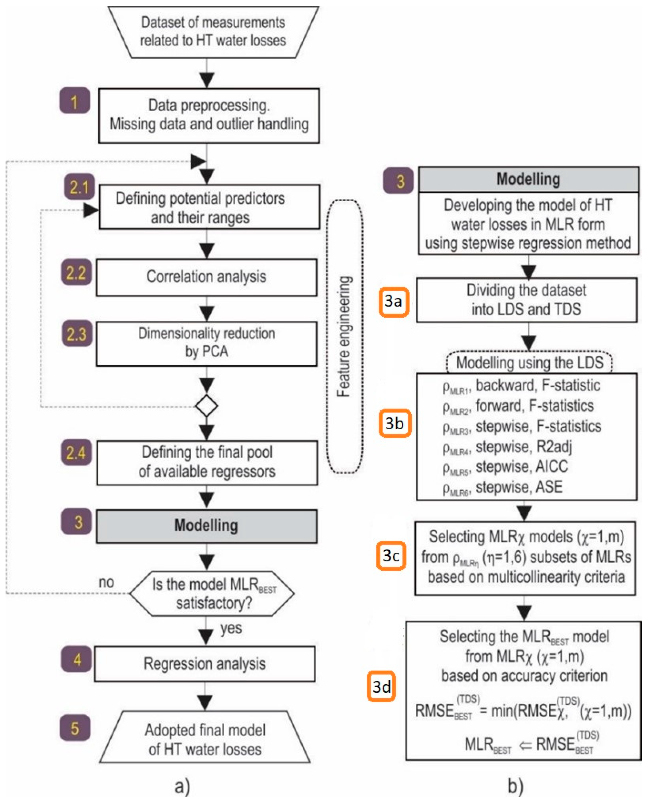
For statistical modeling of water losses and seepage in hydraulic tunnels, we proposed the methodology shown in schematic view in Figure 1. Key features of the proposed methodology are described in the following sections.

3.1. Data Preprocessing and Feature Engineering

The collected dataset consisted of various data related to HT water losses, including measurements of water losses in the tunnel, temperature of concrete, temperature of water and rock, opening and closing of cracks, groundwater levels, etc. Regression models are very sensitive to the occurrence of outliers and missing values in the data. Therefore, the processes of outlier detection and handling, and possible missing data imputation are of crucial importance. This is considered in the first part of the methodology (Figure 1, block 1).

The second part of the methodology relates to feature engineering (Figure 1, block 2). Feature engineering is the act of extracting features from raw data and transforming them into formats that are suitable for predictive modeling [25]. Feature engineering encompasses several stages in our methodology. Building adequate predictive models involves proper selection of predictors and dependent variables and determining valid value intervals for these variables (2.1). Correlation analysis (2.2) is of great importance in this process, because it provides a basis for proper selection of input and output variables, and their potential regressors [19]. Modeling HT water losses involves choosing regressors from a large pool of possible candidate predictors, of which only a few are likely to be important. In our methodology, the dimensionality reduction paradigm is realized through PCA (2.3). The key idea here, as explained in Section 2.1, is to replace redundant features with a few new features that adequately summarize the information contained in the original feature space. In our methodology, PCA consists of three main steps, which are briefly described in the following three paragraphs.

In the first step, data suitability for PCA is assessed in terms of sampling adequacy and strength of the relationship among the variables. Sampling adequacy is assessed based on sample size and Kaiser–Meyer–Olkin (KMO) test of sampling adequacy [26]. The strength of the relationship among the variables is assessed based on examining the correlation matrix and Bartlett’s test of sphericity [27].

In the second step, the number of principal components to be extracted is selected. Deciding on the number of principal components is a considerable challenge in using PCA. In our methodology, three well-known methods are available to assist in this decision: Kaiser’s criterion [26], Cattell’s scree test [28], and Horn’s parallel analysis [29].

In the third step, the principal components are subjected to rotation to gain a better understanding and interpretation of the data. Here, rotation refers to the post-processing of PCA results to obtain a so-called ‘simple structure’ [30], where the division of variables into separate components is more easily interpretable. Two general types of rotation are available: orthogonal, where the new principal axes are also orthogonal to each other, and oblique where the new principal axes are not required to be orthogonal. Our methodology suggests the application of the most frequently used rotation methods: the Varimax method, and the direct Oblimin method, as the most commonly used orthogonal and oblique rotation methods, respectively. A comparison of these rotation methods is given in [18].

Regression models are very sensitive to multicollinearity and singularity, so methodology stages 2.2 and 2.3 are necessary to avoid the pitfalls of model overfitting. Based on previous stages the final pool of candidate regressors is defined in stage 2.4. Candidate regressors are derived by various mathematical transformations of physical quantities that describe the processes related to HT. Furthermore, solving the complex issue of feature engineering can be supported by elements of descriptive statistics and probability distribution laws of physical quantities upon which water losses and seepage depend. The methodological steps in the second stage are often implemented in several iterative steps.

3.2. Modelling

A key issue in creating the model in the form of multiple linear regression (Figure 1, block 3) is the selection of appropriate regressors, considering both the number and type of regressors. To solve this problem, we engaged the method of stepwise regression. In an iterative procedure, the techniques from this method performed automated entering and removing of regressors, thus creating optimal regression models.

At this stage, we defined the following steps:

• Dividing the available data into subgroups: learning dataset (LDS) and test dataset (TDS), according to the given ratio (3a);
• Generating regression models based on LDS during the iterative procedure, using the stepwise regression method with multiple model selection methods: backward, forward, and stepwise (3b). Each of these methods employs additional criteria for entry and removal of regressors. The backward method starts with all regressors in the model, and iteratively performs the removal of regressors based on the criterion of F-statistic and corresponding p-values (probability of F), until no further regressors can be removed without a statistically significant loss of accuracy. This method produced the subset of regression models ${\rho }_{\mathrm{MLR}1}$. The forward method starts with zero regressors in the model, and iteratively performs entry of regressors, also based on the criterion of F-statistic and their p-values. The procedure stops when there are no variables that meet the entry criterion and generates the subset of regression models ${\rho }_{\mathrm{MLR}2}$. The stepwise method is a combination of the backward and forward selection methods. This method terminates when no more regressors are eligible for entry or removal based on the chosen criterion. In our methodology, the stepwise method generates four subsets of MLR models (${\rho }_{\mathrm{MLR}3}$, ${\rho }_{\mathrm{MLR}4}$, ${\rho }_{\mathrm{MLR}5}$, ${\rho }_{\mathrm{MLR}6}$), based on four different criteria for entry and removal of regressors. These criteria are: F-statistic (F-statistic maximum for entry, F-statistic minimum for removal), maximum adjusted coefficient of determination R², minimum corrected Akaike information criterion (AICC), and minimum average squared error over the overfitting prevention data (ASE). The mentioned criteria are explained in detail in [31];
• Selecting the best MLR model of HT water losses, from MLRχ models $\chi =1,m$, based on the chosen accuracy criterion (3d). Various indicators can be selected as criteria for assessing model accuracy. One of them is the root mean squared error (RMSE). In our methodology, RMSE for the test dataset, ${\mathrm{RMSE}}^{\left(\mathrm{TDS}\right)}$, was chosen as the accuracy criterion, and is calculated according to (6):

$${\mathrm{RMSE}}^{\left(\mathrm{TDS}\right)}= \sqrt{\frac{{{\displaystyle \sum }}_{i=1}^n{(q_i-{\widehat{q}}_i)}^2}{n}},$$

(6)

where $q_i$ and ${\widehat{q}}_i$ represent the measured and predicted values of total water losses in HT for the ith record from the TDS, respectively. The model with the ${\mathrm{RMSE}}^{\left(\mathrm{TDS}\right)}$, calculated according to (7):

$${\mathrm{RMSE}}_{\mathrm{BEST}}^{\left(\mathrm{TDS}\right)}=\mathit{min}({\mathrm{RMSE}}_{\chi }^{\left(\mathrm{TDS}\right)},\chi =1,m),$$

(7)

was chosen as the best model, denoted as MLR_BEST.

If MLR_BEST is satisfactory, in comparison to some previously developed reference model of HT water losses, in terms of complexity and accuracy, or some other criteria arbitrarily chosen by the researcher, our methodology follows up with the regression analysis activity. Otherwise, we should return to block 2, and repeat the methodology stages, starting with (2.1), redefining the pool of potential predictors and their ranges, and/or redefining principal components in (2.3).

3.3. Regression Analysis

Detailed performance indicators of generated models, such as confidence intervals, prediction intervals, significance and confidence intervals of regression coefficients, and other indicators of interest, are obtained by regression analysis for the chosen model, MLR_BEST (Figure 1, block 4).

4. Case Study

4.1. Description

In this paper, the hydraulic tunnel of the PSHPP “Bajina Bašta” was analyzed (Figure 2). This tunnel is part of the PSHPP “Bajina Bašta” and was built in the period from 1977 to 1983. During periods of electricity surplus in the energy system of the Republic of Serbia, the supply and drainage hydraulic tunnel serve to pump water from the reservoir of HPP “Bajina Bašta” on the river Drina to the upper reservoir, lake “Lazići”, located in the Tara mountain (Figure 3). On the other hand, when there is a need for electricity, the water goes through the HT to the aggregates of the PSHPP “Bajina Bašta”. The installed capacity of the PSHPP is 600 MW. The tunnel has a circular cross-section with a diameter of 6.30 m, the tunnel’s length is 8030 m, and it has a drop of 4.5‰ (Figure 3). The circular cross-section of the surge tank is 12 m in diameter. Under operating conditions, the maximum hydrostatic pressure in the tunnel can be up to 1.3 MPa.

4.2. Measurements in the Tunnel

In the hydrotechnical tunnel measurements of the temperatures of concrete and water in the tunnel, the water level in the upper reservoir, the water level in the piezometers, and measurements of the width of the crack openings in the tunnel’s concrete lining are conducted approximately two times per month. Measurements of the total water losses are conducted 2–4 times per year depending on the weather conditions and the tunnel exploitation regime.

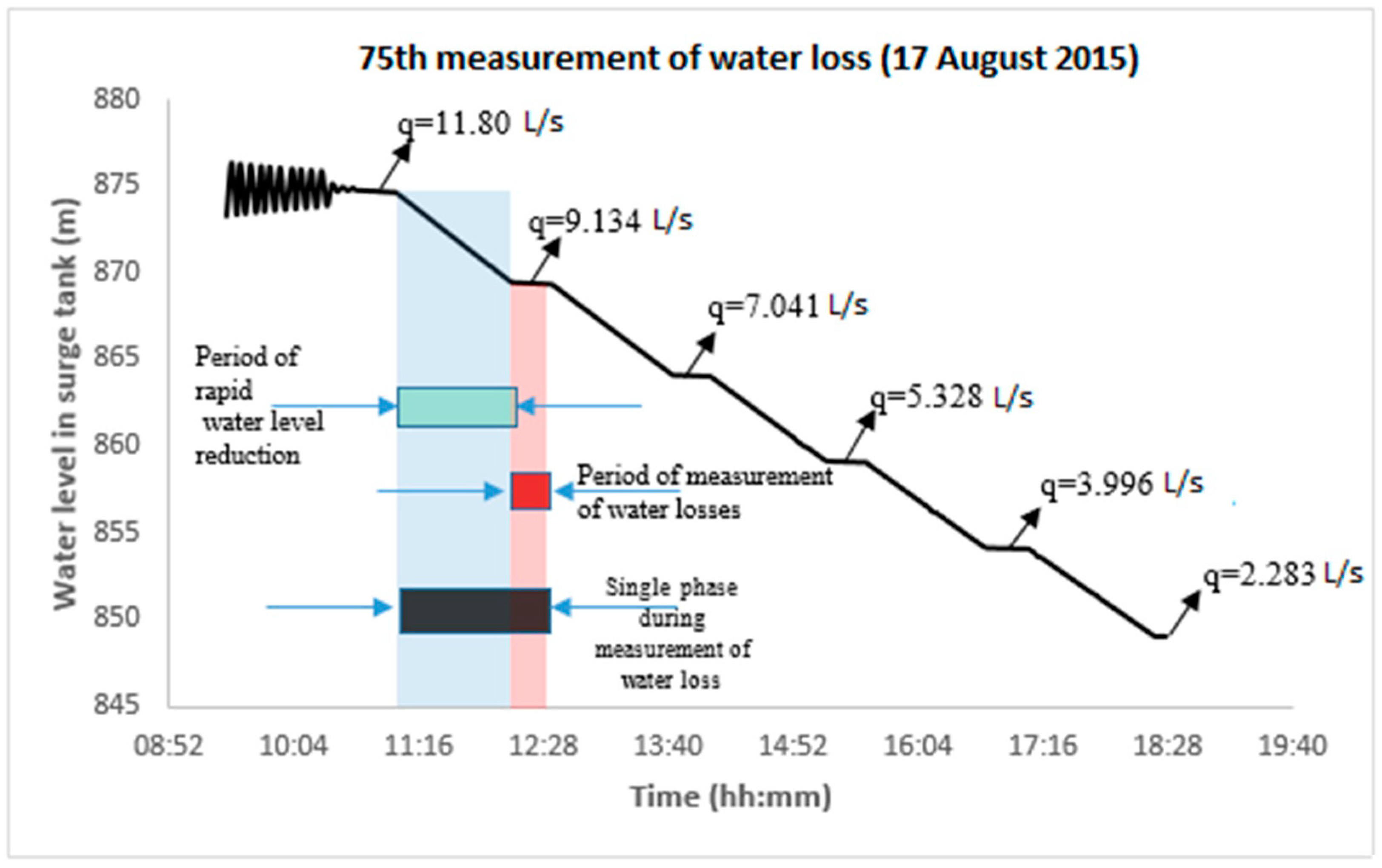
Measurement of total water losses is carried out under conditions when the tunnel is closed both at the entrance building at the upper reservoir and at the outlet towards the pipeline. One session of measurements of total water loss is performed in several phases. A single phase includes the rapid reduction of the water level in the surge tank down to some level, $H_i$, and then, a measurement step. In the measurement step, it is measured how much the water level $H_i$ has lowered in the observed time interval. The decrease in water level is the result of water loss from the tunnel. At the end of the measurement step, the water level is $H_{i+1}$. Based on the difference, $H_i-H_{i+1}$, the resulting volume of lost water $\mathsf{\Delta }V$ from the tunnel is obtained according to (8) [4].

$$\mathsf{\Delta }V=\left(H_i-H_{i+1}\right)\cdot \frac{D^2\pi }{4},$$

(8)

The total water loss is calculated according to (9):

$$q=\frac{\mathsf{\Delta }V}{\mathsf{\Delta }t},$$

(9)

where $q$ [L/s], $\mathsf{\Delta }V$ [l], and $\mathsf{\Delta }t$ [s] are the total water loss, water volume decrease in the surge tank with a circular cross-section (diameter D = 12.0 m), and time interval, during a single measurement step, respectively. The measuring is stopped when the total water loss $q$ becomes negative—$\mathsf{\Delta }V$ becomes negative, i.e., water volume in the surge tank starts increasing and water loss turns into water inflow. The duration of one measurement step is usually 30 min. According to the same principle, the procedure repeats in the next phases in the session.

Figure 4 shows a diagram of water level change in the surge tank during one session of total losses measurement (in this case, the 75th session, 17 August 2015).

During the session of measurement of total water losses, measurements of concrete temperature on the extrados of the concrete lining, water temperatures, width of the crack openings, water level in the upper reservoir, and water level in piezometers are also measured at the same time.

For measuring the temperatures of the water and the concrete, thermometers are installed in the tunnel lining (on the extrados and intrados of the tunnel). The instruments are isolated from the effects of water and the measurements are conducted twice a month via a portable measuring station. For measuring the width of the crack openings electroacoustic deformeters are installed in the concrete in the zone of the crack. The instruments are isolated from the effects of water and the measurements are conducted twice a month via a portable measuring station (outside the tunnel).

4.3. Dataset

During the exploitation of the tunnel, for the period from 1983 to 2017, 79 measurement sessions of total water loss were carried out. In this paper, data for the period from 2005 (year of the last tunnel reparation and injection) to 2017 were analyzed—measuring sessions of total water loss from 50 to 79, which generated 180 data measurement records. For the considered input and output variables, the following symbols were introduced: $H_r$—water level in the upper reservoir, $H_{p3}$ and $H_{p4}$—water levels in piezometers P₃ and P₄, respectively, $T_c$—concrete temperature on the extrados of the concrete lining, $T_w$—temperature of water, $H_{st}$—average water level in the surge tank for one measurement step, $c{r}_3$ and $c{r}_4$—width of crack openings at the measuring points M0P-3 and M0P-4, respectively, and $q$—total water losses from the tunnel. In addition to these variables, variable $t$, which represents the elapsed time in months from the date of the last tunnel reparation and injection performed in 2005, is introduced. The variable $t$ considers the impact of rheology on the aging and deterioration of concrete as well as possible changes in geology that can lead to irreversible processes and have a lasting effect on total water losses in the tunnel.

The elements of descriptive statistics of measured values are given in

Table 1. Descriptive statistics of measured values for measurement sessions 50–79.

	${\mathit{H}}_{\mathit{r}}$	${\mathit{H}}_{\mathit{p}3}$	${\mathit{H}}_{\mathit{p}4}$	${\mathit{T}}_{\mathit{c}}$	${\mathit{T}}_{\mathit{w}}$	${\mathit{H}}_{\mathit{s}\mathit{t}}$	$\mathit{c}{\mathit{r}}_3$	$\mathit{c}{\mathit{r}}_4$	$\mathit{t}$	$\mathit{q}$
	[m a.s.l.]	[m a.s.l.]	[m a.s.l.]	[°C]	[°C]	[m a.s.l.]	[mm]	[mm]	[months]	[L/s]
Min.	854.380	862.950	862.780	2.520	3.190	831.825	−0.722	-0.033	4.0	−0.190
Max.	880.260	879.650	879.550	14.560	21.000	879.996	0.129	0.424	139.0	25.511
Average	874.660	874.379	873.697	9.100	11.730	860.617	−0.480	0.103	72.0	9.845
St. dev.	5.116	3.793	3.888	3.105	4.377	10.640	0.224	0.122	41.3	5.176

.

4.4. Correlation Analysis and PCA of Total Water Losses

4.4.1. Correlation Analysis

A correlation analysis was performed for the available dataset of measuring sessions total water loss of 50–79. The values of Pearson’s correlation coefficient are given in

Table 2. Correlation matrix for considered input and output variables for the period 2005–2017.

	${\mathit{H}}_{\mathit{r}}$	${\mathit{H}}_{\mathit{p}3}$	${\mathit{H}}_{\mathit{p}4}$	${\mathit{T}}_{\mathit{c}}$	${\mathit{T}}_{\mathit{w}}$	${\mathit{H}}_{\mathit{s}\mathit{t}}$	$\mathit{c}{\mathit{r}}_3$	$\mathit{c}{\mathit{r}}_4$	$\mathit{t}$	$\mathit{q}$
	[m a.s.l.]	[m a.s.l.]	[m a.s.l.]	[°C]	[°C]	[m a.s.l.]	[mm]	[mm]	[months]	[L/s]
$H_r$
$H_{p3}$	0.482
$H_{p4}$	0.491	0.873
$T_c$	0.355	0.334	0.179
$T_w$	0.310	0.340	0.148	0.840
$H_{st}$	0.441	0.258	0.264	0.129	0.127
$c{r}_3$	−0.384	−0.452	−0.328	−0.903	−0.875	−0.164
$c{r}_4$	−0.384	−0.433	−0.314	−0.898	−0.876	−0.167	0.995
$t$	−0.230	0.165	0.128	−0.130	−0.110	−0.072	0.060	0.060
$q$	0.164	−0.066	−0.033	−0.257	−0.291	0.758	0.304	0.309	0.015

.

The correlation coefficient values in Table 2 indicate that most of the input variables can be considered linearly independent since most correlation coefficient values are less than 0.7 [17].

The correlation coefficient between variables $H_{p3}$ and $H_{p4}$ is 0.873, which indicates a strong correlation. This is to be expected because the piezometers are at a close distance and under the same geological conditions. The concrete temperature on the extrados of the concrete lining $T_c$ is in a strong correlation (0.840) with the water temperature $T_w$, which is reasonable because the temperature is measured in the interior and exterior of the concrete lining, so these temperatures are interdependent. Variables $T_c$ and $T_w$ are in a very strong negative linear correlation with the sizes of crack openings $c{r}_3$ and $c{r}_4$. This can be explained by the fact that at high temperatures there is an increase in the expansion of concrete, and consequently the cracks are closed, and in the case of lower temperatures, the concrete contracts and the cracks open up. The average water level during a single measurement step, $H_{st}$ has a strong influence on total water loss, the coefficient of correlation being 0.758. Variables $c{r}_3$ and $c{r}_4$ are in positive correlation with variable $q$, because the increase in crack openings leads to an increase in total water losses.

The increase in water and concrete temperature leads to expansion of the tunnel’s concrete lining, thereby reducing the size of crack openings which leads to a reduction of water losses from the tunnel. For these reasons, concrete and water temperatures are in negative correlation with the variable $q$, with the correlation coefficients being −0.257 and −0.291, respectively.

Since the measurement of total losses is carried out at a constant water level in the upper reservoir, in piezometers, and under variable conditions in the surge tank, it is therefore expected that the coefficient of correlation between $H_r$, $H_{p3}$, and $H_{p4}$ on q is small. Although these variables individually have little linear effect on the output (the correlation coefficients are significantly lower than 0.3), in order to initially include a more comprehensive set of measured quantities, their interaction effects, and derived variables, the mentioned variables are taken into account for further consideration.

Based on the correlation analysis, it can be concluded that some input variables are strongly linearly dependent and should not be used as such for modeling, because of the problem of multicollinearity [32]. In order to reduce multicollinearity, simplify the model of HT water losses (Ockham’s razor) [33], and enable better physical interpretation of the model by dimensionality reduction, PCA was carried out.

4.4.2. PCA Results

A set of 9 variables, described in 4.3, was subjected to PCA using R software [34]. Firstly, the suitability of data for PCA was assessed. The number of samples was 156, which exceeds the minimum recommended sample size of 150 [18]. The value of the KMO index was 0.772, which exceeds the minimum recommended value of 0.6, and indicates sampling is adequate [18]. Most correlation coefficients (23 out of 36) in the correlation matrix were above 0.3 [18] and Bartlett’s test of sphericity reached statistical significance (p < 0.05) [27], indicating the factorability of the correlation matrix.

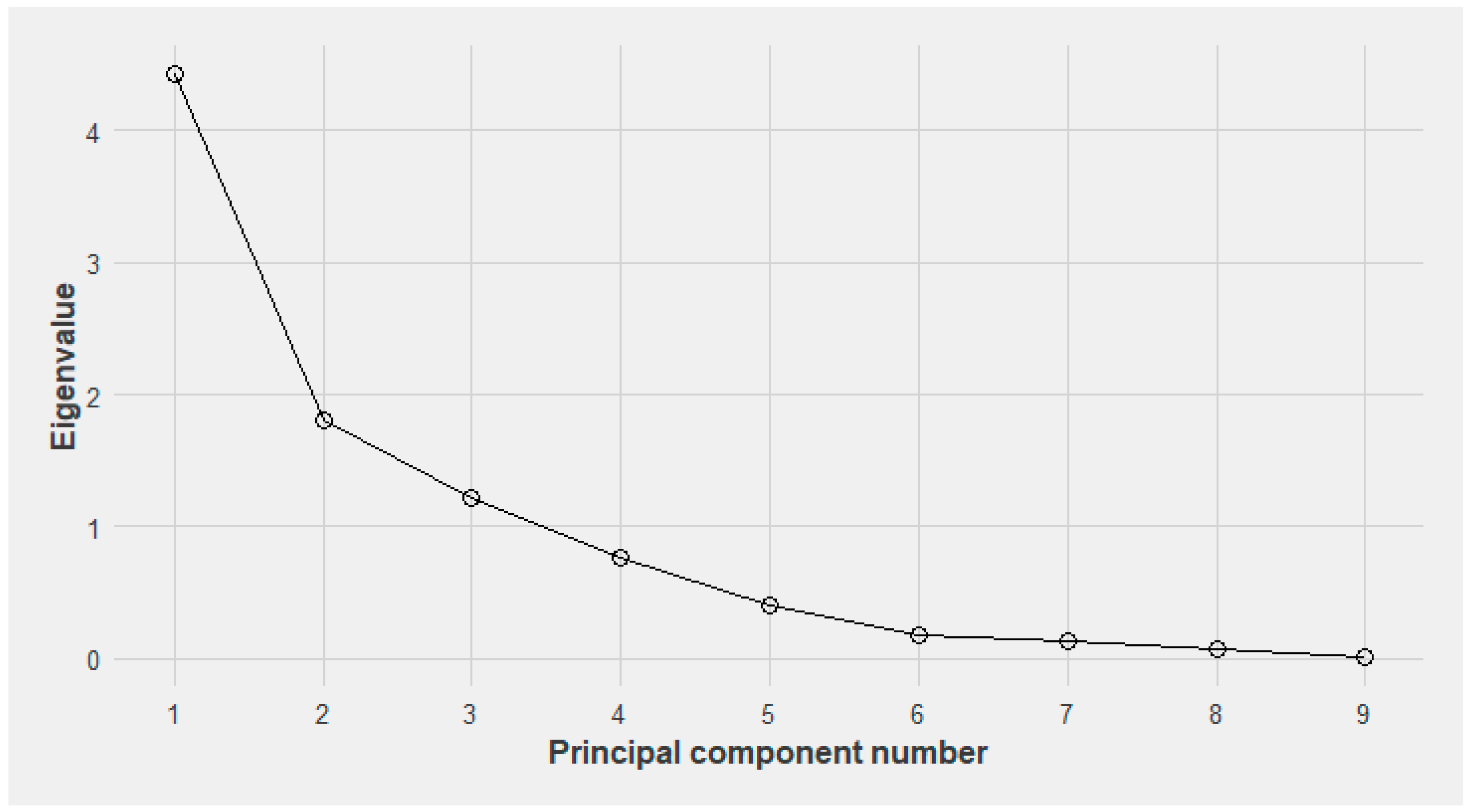
In the second step, PCA analysis revealed the presence of 3 components with eigenvalues exceeding 1 (Kaiser’s criterion) [26], which explain 49.13%, 20.01%, and 13.58% of the variance respectively, accounting for 82.72% of total variance. Cattell recommends retaining all components above the elbow or break in the plot (Figure 5), as these factors contribute the most to the explanation of the variance in the data set [28]. Based on Cattell’s test it has been found that reduction to the 2, 5, or 6 principal components can be considered.

Horn’s parallel analysis involves comparing the size of the eigenvalues with those obtained from a randomly generated data set of the same size. Only components with eigenvalues that exceed the corresponding values from the random data set are retained [29]. The results of the parallel analysis, shown in

Table 3. Results of Horn’s parallel analysis.

PC	PC Eigenvalues	Eigenvalues Obtained by Horn’s Parallel Analysis	Decision
1.	4.422	1.3549	accept
2.	1.801	1.2326	accept
3.	1.222	1.1374	accept
4.	0.759	1.0594	reject
5.	0.404	0.9872	reject
…	…	…	…
9	0.050	0.6734	reject

, indicate three components whose eigenvalues exceed the corresponding threshold values obtained using an equally sized matrix of random numbers (9 variables and 162 records). Horn’s parallel analysis was carried out using the Monte Carlo PCA for parallel analysis software [35].

Although Kaiser’s criterion and Horn’s parallel analysis suggest a three-component solution, accounting for 82.72% of total variance, we arbitrarily selected a five-component solution based on Cattell’s test, in order to retain more information about the process of generating water losses in the HT and facilitate a more accurate model of water losses. The five-component solution explains a total of 94.61% variance, with component contributions of 49.13%, 20.01%, 13.58%, 8.44%, and 4.45%, respectively.

In the third step, several rotation methods were performed. Finally, the direct oblimin rotation method was chosen as appropriate, enabling the following PC interpretations: $T_{wcc}$—which includes water temperature, concrete temperature, and cracks opening $hP$—which includes the influence of water level in the piezometers, $\overline{t}$—which represents time, ${\overline{H}}_{st}$—which represents water level in the surge tank, and ${\overline{H}}_r$—which represents water level in the upper reservoir.

Table 4. PC correlation matrix.

	${\mathit{T}}_{\mathit{w}\mathit{c}\mathit{c}}$	$\mathit{h}\mathit{P}$	$\overline{\mathit{t}}$	${\overline{\mathit{H}}}_{\mathit{s}\mathit{t}}$	${\overline{\mathit{H}}}_{\mathit{r}}$
$T_{wcc}$
$hP$	0.312
$\overline{t}$	−0.085	0.161
${\overline{H}}_{st}$	0.147	0.261	−0.067
${\overline{H}}_r$	0.357	0.484	−0.229	0.436

shows correlation coefficients between selected PCs.

It can be seen from Table 4 that some components are linearly independent of each other because the correlation coefficients are less than 0.3, and some components have mild linear dependence.

4.4.3. Defining the Pool of Candidate Regressors

In accordance with our methodology, after obtaining the principal components, we defined the pool of candidate regressors. In the modeling of total water losses, PCs can be roughly divided into several groups, based on the physical nature of the input variables: the effects of hydrostatic pressure, the effects of temperature and size of crack openings, and the effects of time (aging, which is considered to be irreversible). The effects of hydrostatic pressure variation are usually represented by polynomials, power, and exponential or logarithmic functions, depending on the water level [21]. In our case study, for hydrostatic principal components (${\overline{H}}_{st}$, ${\overline{H}}_r$, $hP$) we arbitrarily opted for polynomial terms of the first and second order. As described in the previous section, $T_{wcc}$ includes the water temperature, concrete temperature, and size of crack openings, and the authors have chosen to express its potential predictive effect on total water losses in polynomial and exponential form. It can be assumed that water losses increase with the time elapsed since the last tunnel reparation date. This aging effect can also be interpreted in the following way—the effect of the last tunnel reparation on water losses from the tunnel exponentially decays with time. This long-time behavior is modeled by a negative exponential drift regressor, $-e^{-\overline{t}/k}$, where $\overline{t}$ is time in months elapsed since the last reparation date, and $k$ is a scaling factor, which cannot be determined a priori. Several regressors with different values of $k$ (1, 2, 4, and 10) were placed in the pool of regressors, with an assumption that the stepwise regression method will make an appropriate choice of regressors during the modeling process of water losses. During the application of PCA rotation methods, we did not achieve a simple structure (Table 4). This shortcoming is dealt with in the modeling stage of our methodology (Figure 1, block 3), with the use of interaction terms in forms $T_{wcc}{\overline{H}}_{st}$, $T_{wcc}{}^2{\overline{H}}_{st}$, and $T_{wcc}{\overline{H}}_{st}{}^2$.

Based on previous considerations, an initial set of regressors was created, using the five principal components ($T_{wcc}$, $hP$, $\overline{t}$, ${\overline{H}}_{st}$, ${\overline{H}}_r$) (

Table 5. Potential regressors for the water losses model.

Type	Single Terms					Interaction Terms
Principal components	${\overline{H}}_{st}$	${\overline{H}}_r$	$hP$	$T_{wcc}$	$\overline{t}$
Regressors	${\overline{H}}_{st}$${\overline{H}}_{st}{}^2$	${\overline{H}}_r$${\overline{H}}_r{}^2$	$hP$$h{P}^2$	$T_{wcc}$$, T_{wcc}{}^2$$e^{-T_{wcc}}$	$e^{-\overline{t}}$$, e^{-\overline{t}/2}$$e^{-\overline{t}/4}$$, e^{-\overline{t}/10}$	$T_{wcc}{\overline{H}}_{st}$$, T_{wcc}{}^2{\overline{H}}_{st}$$T_{wcc}{\overline{H}}_{st}{}^2$

).

4.5. Model of Total Water Losses in the HT Based on Principal Components

Based on the created pool of regressors, the development of the HT total water losses model was performed in accordance with the strategy described in Section 3 and shown in Figure 1, block 3. The process of modeling was based on the measurements described in Section 4.3. From the total number of records (180), 156 were used for modeling (LDS—learning dataset), and 24 records were used to test the model (TDS—test dataset) (Figure 1(3a)). The TDS, consisted of records from the last four measurement sessions (76–79) of total water losses, in period 2015–2017, i.e., from the last period of HT monitoring.

The automated software procedure, in accordance with the stepwise paradigm and numerous stepwise regression method variations described in Section 3.2, resulted in several MLR models of HTs total water losses which are stored in appropriate subsets of MLR models from ${\rho }_{\mathrm{MLR}1}$ to ${\rho }_{\mathrm{MLR}6}$ (Figure 1(3b)). The numerous models obtained from the iterative procedures are not shown due to their size. The most accurate model, MLR_Best, which satisfies the condition of non-multicollinearity, was chosen as appropriate (Figure 1(3d)), from the previous selected set of non-multicollinear regression models ($\mathrm{MLR}\chi , \chi =1, \mathrm{m}$) (Figure 1(3c)). The obtained model was the results of the stepwise selection method and the AICC criteria for entry/removal of regressors. AICC is based on the likelihood of the training set given the model and is adjusted to penalize overly complex models [36]. The coefficient of multiple determination ($R^2$), adjusted coefficient of multiple determination ($R_{adj}^2$) and RMSE were selected as measures of selected model accuracy. The values of these indicators were $R^2=0.94014$, $R_{adj}^2=0.87386$ and RMSE_LDS = 1.8842 L/s.

The final adopted regression model, with all parameters and results of regression analysis, according to Section 3.3, is shown in

Table 6. Parameters of the final adopted MLR model of HTs total water losses.

Regressors	Unstandardized Coefficients		Standard. Coeff.	t	p Value	95% Confidence Interval for B		Correlations		Collinearity Statistics
	B	Std. Error	β			Lower Bound	Upper Bound	Partial	Part	Toler.	VIF
Constant	10.209	0.321		31.76	0.000	9.575	10.844
${\overline{H}}_{st}$	4.425	0.160	0.855	27.64	0.000	4.109	4.741	0.903	0.814	0.907	1.103
$T_{wcc}$	−1.787	0.177	−0.345	−10.09	0.000	−2.136	−1.438	−0.610	−0.298	0.743	1.347
$hP$	−1.151	0.184	−0.222	−6.25	0.000	−1.514	−0.787	−0.430	−0.184	0.686	1.458
$T_{wcc}{\overline{H}}_{st}$	−1.169	0.155	−0.266	−7.55	0.000	−1.475	−0.863	−0.499	−0.222	0.698	1.433
$e^{-\overline{t}}$	−0.663	0.109	−0.185	−6.10	0.000	−0.878	−0.449	−0.422	−0.180	0.939	1.064
${\overline{H}}_{st}{}^2$	0.451	0.147	0.100	3.08	0.002	0.162	0.740	0.228	0.091	0.817	1.223
$T_{wcc}{}^2$	0.408	0.171	0.094	2.39	0.018	0.071	0.746	0.179	0.070	0.560	1.787

.

The analytic form of the MLR model of HTs total water losses, based on PCs, is presented in Equation (10).

$$\begin{gathered} q=10.20945+4.22495\cdot {\overline{H}}_{st}-1.78695\cdot T_{wcc}-1.15069\cdot hP \\ -1.16897\cdot T_{wcc}\cdot {\overline{H}}_{st}-0.66310\cdot e^{-\overline{t}}+0.45082\cdot {\overline{H}}_{st}{}^2+0.40840\cdot T_{wcc}{}^2, \end{gathered}$$

(10)

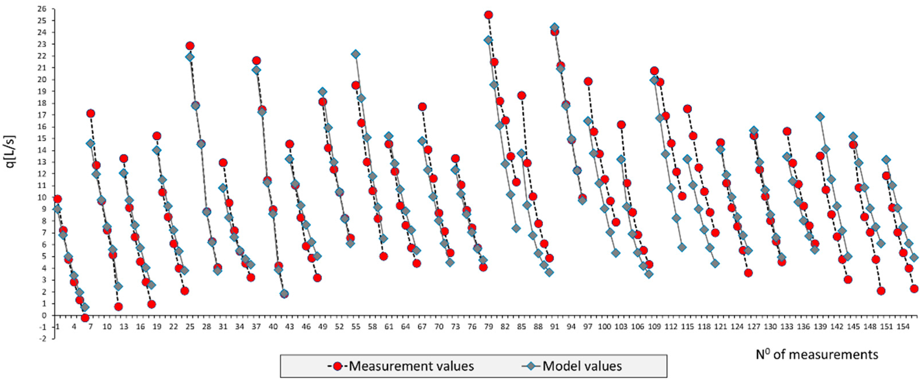
The measured and predicted values of total water losses in the HT, based on the LDS, for the period 2005–2015 are shown in Figure 6.

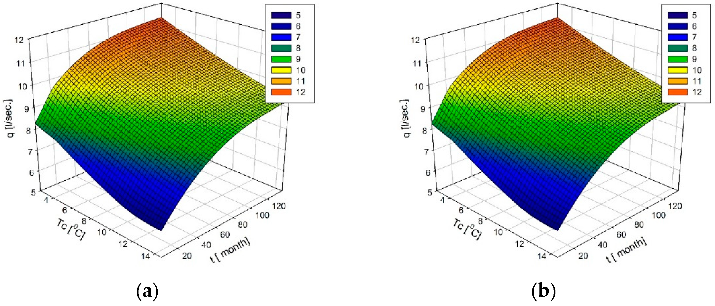
Various 3D surface plots can also represent the adopted mathematical model of HT total water losses. Such visualizations (Figure 7) can be useful for the interpretation of physical quantity effects, and the significance of individual predictors. In the diagrams shown, in addition to the predictors shown on the axes, all other predictors are constant and equal to their mean values.

The diagram in Figure 7a presents a surface showing an increase in total water losses in HT of PSHPP “Bajina Bašta”, as a function of time and temperature in the extrados of the concrete lining. It can also be seen that the effect of reparation on water losses from the tunnel is the largest in the first few years after the tunnel reparation was carried out in 2005. After that, this effect slowly dissipates, following an exponential law. The diagram in Figure 7b presents the surface showing that water losses increase with the increasing water level in the surge tank and with the reduction of concrete temperature.

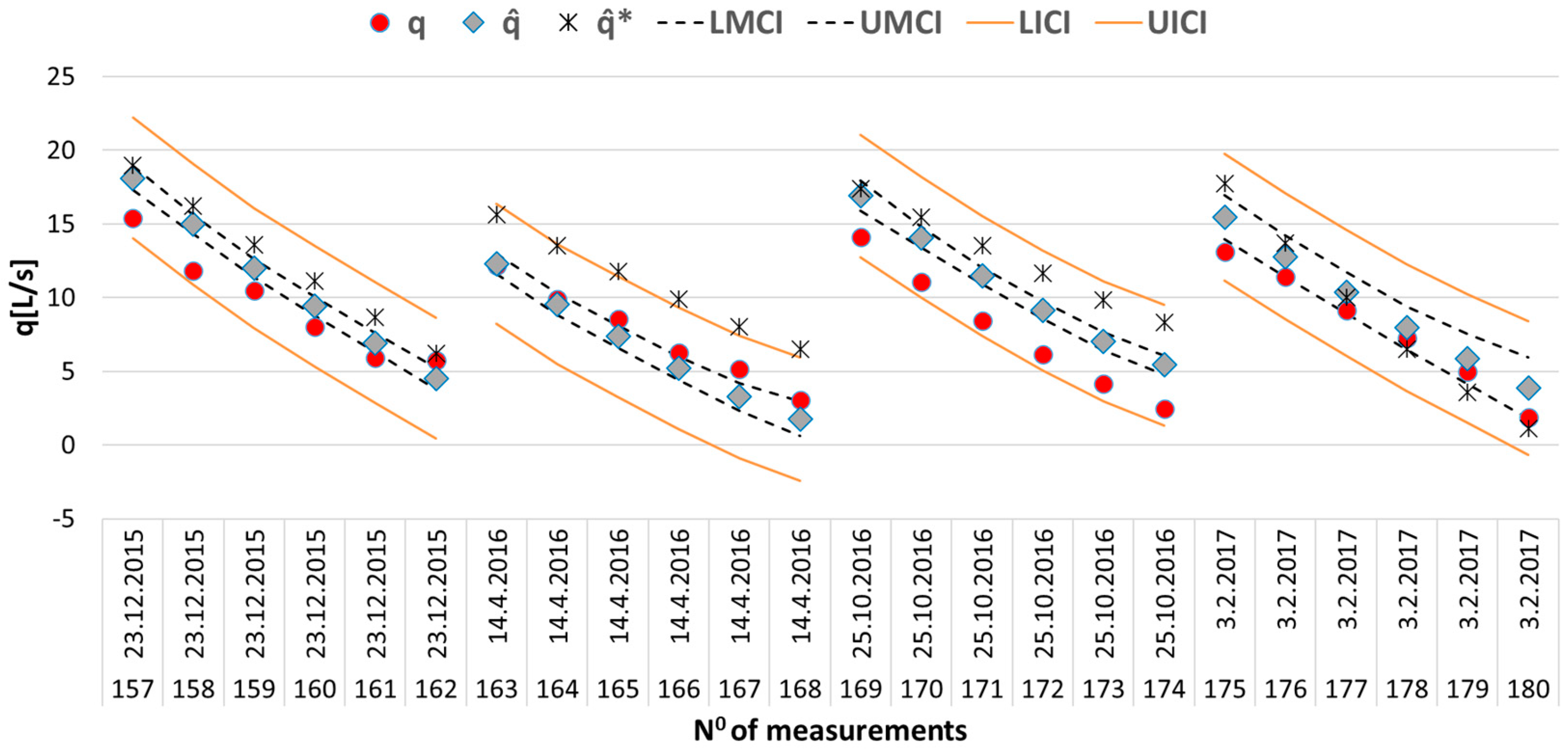
The final adopted model of HT total water losses was verified using the dataset that was not used in the model development process. Figure 8 shows diagrams of predicted and measured values of total water losses during the test period.

In Figure 8, $q$ represents the measured values, $\widehat{q}$ represents the model values according to the model (10) in this paper, and $\widehat{q}*$ represents the model values of water losses according to the model given in paper [4]. Test sessions refer to the last four sessions, sessions 76–79, i.e., measured values 157–180. $LMCI$, $UMCI$, $LICI$, and $UICI$ represent the lower (L) and upper (U) limits of the confidence intervals for the expected mean (M) and individual values (I) of the model (10). The accuracy of the model for the test period is RMSE_Test = 2.0161 L/s.

Model (10) is additive, and Figure 9a shows the aggregate effects of regressors grouped by their physical context. The additive component $aHst$ represents the sum of linear and quadratic hydrostatic effects ($H_{st}$ and $H_{st}^2$), $aTwcc$ represents the sum of linear ($T_{wcc}$) and quadratic ($T_{wcc}^2$) thermal and size of crack openings effects, while component $ahP$ is the sum of hydrostatic effects of groundwater measured by piezometers P₃ and P₄. Component $T_{wcc}\cdot H_{st}$ represents the interaction effects of appropriate PCs, and $t$—encompasses the effect of rheology on aging and deterioration of concrete ($e^{-t}$).

5. Discussion

The adopted model includes 94.61% variance of water losses from the tunnel. Based on the Tolerance and VIF columns (Table 6), it can be seen that the adopted model has no problems with multicollinearity (for each of the regressors: Tolerance > 0.1 and VIF < 10). The Standardized Coefficient column (β) shows the contribution of individual regressors to the entire model. The linear impact of the hydrostatic pressure on the water level in the surge tank (${\overline{H}}_{st}$) dominantly affects water losses (0.855). This dominant effect is followed by the thermal effects (temperatures of water and concrete) coupled with cracks (−0.345), water height in piezometers (−0.222), interaction effects of temperature, size of crack openings, the water level in the surge tank ($T_{wcc}{\overline{H}}_{st}$) (−0.266), and the exponential influence of time since the last repair (−0.185). Standardized beta values indicate the number of standard deviations that scores in the dependent variable would change if there was one standard deviation unit change in the predictor [17]. In model (10), if we could increase the water level in the surge tank (${\overline{H}}_{st}$) by one standard deviation (which is 10.64 m a.s.l., from the descriptive statistic in Table 1) the total water loss ($q$) would be likely to increase by 0.855 standard deviation units (which is 4.42548 L/s, for $\sigma =5.176$ L/s, according to Table 1). The p-value column shows that each regressor in the model gives a unique contribution to the model (for each regressor, p-value associated with the F-statistic is less than 0.05). The squared values of semi-partial correlation coefficients (Part) indicate the values of individual regressor contributions to the total variance of the dependent variable. These unique contributions to the $q$ variable variance for the regressors ${\overline{H}}_{st}$, $T_{wcc}$, $hP$, $T_{wcc}$, ${\overline{H}}_{st}$, $e^{-t}$, ${\overline{H}}_{st}^2$, and $T_{wcc}^2$ are 0.6626, 0.0888, 0.0339, 0.0493, 0.0324, 0.0083, and 0.0049, respectively. In other words, the water level in the surge tank contributes 66.26% to the variance of total water losses in HT, temperatures of water. and concrete temperature on the extrados of the concrete lining in the tunnel coupled with cracks, contribute 8.88%, etc. Note that the $R^2$ value for the model (in this case 0.94014, or 94.014% explained variance) does not equal all the squared part correlation values added up (0.8801). This is because the part correlation values represent only the unique contribution of each variable, with any overlap or shared variance removed or partially taken out.

The quality of the adopted model (10) of total water loss in HT of PSHPP “Bajina Bašta” is visualized by the diagram which shows measured and predicted values of total water losses for the LDS (Figure 6). The 3D diagrams in Figure 7 correspond to the physical nature of the tunnel water loss phenomenon, as described above in Section 4.5.

Accuracy indicators for the adopted model, are given in

Table 7. RMSE [L/s] of HTs total water loss.

	LDS	TDS
Model (10) adopted in this paper	1.8842	2.0161
Previous reference model	3.954	3.5983

. For the purpose of model comparison, RMSE values for the previous reference model of HT water losses [1] are also given in Table 7, for the same observation period.

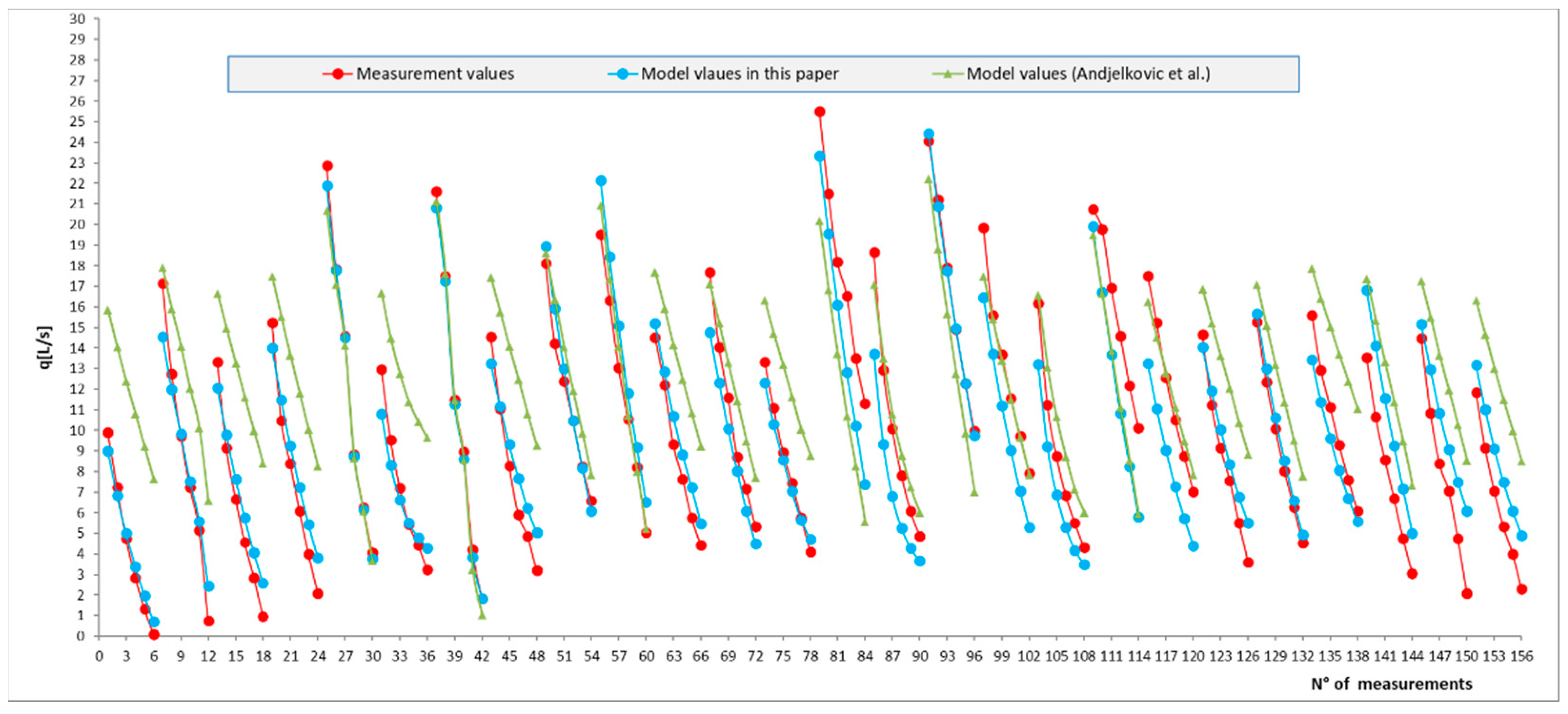
Using the novel methodology for modeling water losses at HT, we obtained the RMSE_LDS of 1.8842 L/s, which is much better than 3.954 L/s obtained by the previous reference model on the same learning dataset. The model in this paper also performs better on the test dataset (2.0161 < 3.5983). The graphical comparison of the mentioned models, for the last four measurement sessions, together with confidence intervals, is given in Figure 8. In Figure 10, the comparison is made between the measured total water losses, the modeled total water losses using the model suggested in this paper (10), and the modeled total water losses using the model suggested by Andjelkovic et al. [4].

Further improvements in the quality of the mathematical model of water loss in the HT of PSHPP “Bajina Bašta” are described in the following two paragraphs.

It should be emphasized that the model developed in this paper also takes into account more input variables (size of crack openings and tunnel aging) than the previous reference model. The sizes of crack openings directly affect the increase or decrease in total water losses, which is important for the quality and accuracy of the proposed model. Consideration of the time component as an input variable gives the possibility of taking into account the irreversible process of concrete and structure aging, but also that, which is most important in the SaFE context, the effect of tunnel reparation on the reduction of total water losses in HT.

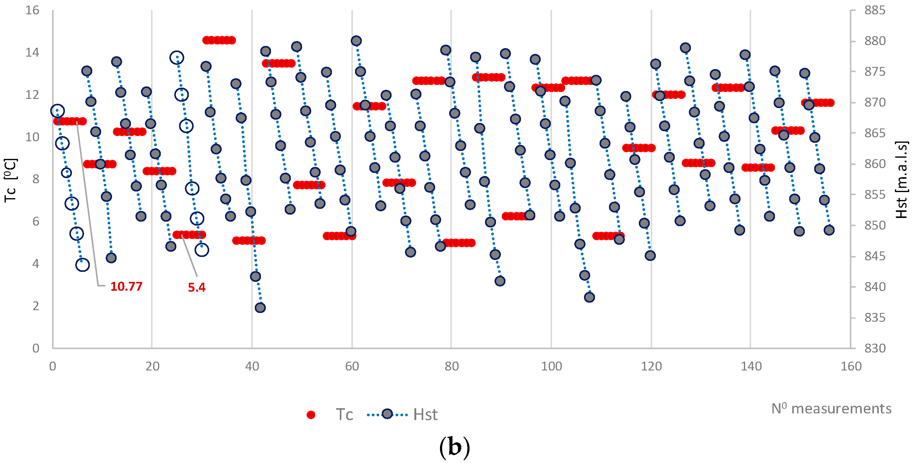
The advantage of the developed model is also the property of additivity, as there is an implicit assumption that the different model (10) regressors affect water losses in the HT additively. The aggregate and individual effects of PCs and regressors derived from them further shed light upon the process of water losses in the HT (Figure 9). For example, for the measurement sessions in which the temperatures of concrete were 10.7 and 5.4 °C (Figure 9b), the thermal effect is inversely proportional to water losses and amounts to −0.73 and 3.31 L/s (Figure 9a). From the SaFE aspect, the exponential influence of time elapsed from last tunnel reparation date in 2005. (predictor t) is particularly interesting. The diagrams shown in Figure 5 and Figure 9a show that the impact of the last tunnel reparation on water losses decreases by the exponential law and becomes negligible after 8–10 years, i.e., 130 measurements, approximately.

The safety of the tunnel cannot be analyzed using the model of total water losses. For this, other methods based on numerical models are needed (FEM, DEM, PDEM, etc.), which were not the subject of research in this paper. For further research, an integral approach can be applied: the usage of numerical and statistical models. When the tunnel is reopened (upon its inspection), it is necessary to record the condition of the tunnel, conduct mapping of all the cracks in the tunnel, categorize the cracks, and form a three-dimensional numerical model that can analyze the behavior of the tunnel with regards to filtration and stress–strain phenomena. After that, a calibration of the numerical model with the total water loss measurements can be conducted, in order to obtain the best correlation between the calculated losses in the model and the measured total losses. This results in a model that takes into account the realistic field conditions and gives the possibility for a safety analysis of the tunnel. However, the use of statistically based models is an economical method that does not demand complex computing resources and know-how. It can be used daily, and it provides a fast assessment of the conditions in the tunnel and its functionality. For more complex analyses of the conditions in the tunnel and its functionality, more complex numerical models that can take into account significant phenomena of tunnel behavior in interaction with water should be used. Additionally, adequate constitutive material models that take into consideration the joints and porosity of the rock mass can be used to calibrate the numerical model more accurately, and therefore have a more realistic model compared to the field conditions.

6. Conclusions

Most pumped-storage hydroelectric power plants in Europe and the world are 30–50 years old. Within these complex hydro-technical facilities, there are HTs where monitoring and forecast of static instability in terms of failure and functional instability in terms of water losses from the tunnel are of enormous significance. The assessment of SaFE indicators in HT is generally conducted in two ways: (a) by emptying the tunnel and conducting physical inspection (b) by mathematical modeling of significant variables in HT with different types of analytical, numerical, statistical, or ML models. The literature review shows that there are not many articles dealing with problems of HT safety and functionality, in particular with problems of water losses from the tunnel. For these reasons, this paper presents a novel methodology for the mathematical modeling of water losses in HT. In addition, the goal was to validate this methodology by building an MLR model of water losses with greater accuracy and reliability, compared to previously developed models of HT water losses.

The methodology in this paper included the following modeling phases: correlation analysis, dimension reduction by PCA, generation of MLR models based on stepwise method, regression analysis, as well as iterative reduction of model complexity achieved by avoiding multicollinearity of the model, thus improving model stability.

A model of HT water losses developed based on the case study was carried out for the hydraulic tunnel at PSHPP “Bajina Bašta”, located on the Drina river, in the Republic of Serbia for the period 2005–2017. The most accurate model, MLR_Best, which satisfies the condition of non-multicollinearity, was chosen as appropriate. A detailed regression analysis indicated that the regressors which have the greatest impact on HT water losses are water level in the surge tank, and the regressor that includes the impact of water temperature, concrete temperature and size of crack openings.

By comparing the model adopted in this paper with other literature for the same tunnel, it was concluded that the new model has better accuracy. It should be emphasized that the model developed in this paper also takes into account more input variables (size of crack openings and tunnel aging) than the previous model.

The analyses of water loss in hydrotechnical tunnels are of great significance because the loss of water implies economical losses, and on the other hand can point out that damages or changes in the tunnel have occurred, which can lead to loss of tunnel stability. Based on the proposed model in this paper, it is possible to determine, in a fast, efficient, and economically acceptable manner, any possible problems in the observed tunnel and provide indications for their resolution. Situations where there are significant deviations between the measured and model predicted values of water losses should demand a more detailed analysis, even including tunnel opening and its thorough inspection. Based on this analysis it can be determined if there is a need for new HT reparation.

Due to the immense importance that the SaFE paradigm for HT has in the PSHPP, the authors intend to further improve the model of total water losses. The improvement of the model would be mostly based on the introduction of new modeling methods, such as artificial neural networks, from which higher model accuracy can be expected.

References

1. Liu, S.; Li, Z. Unloading Behaviors of Shale under the Effects of Water Through Experimental and Numerical Approaches. Int. J. Geomech. 2022, 22, 04022071. [Google Scholar] [CrossRef]
2. Li, Z.; Liu, S.; Ren, W.; Fang, J.; Zhu, Q.; Dun, Z. Multiscale Laboratory Study and Numerical Analysis of Water-Weakening Effect on Shale. Adv. Mater. Sci. Eng. 2020, 2020, 5263431. [Google Scholar] [CrossRef]
3. Roy, D.G.; Singh, T.N.; Kodikara, J.; Das, R. Effect of Water Saturation on the Fracture and Mechanical Properties of Sedimentary Rocks. Rock Mech. Rock Eng. 2017, 50, 2585–2600. [Google Scholar] [CrossRef]
4. Andjelkovic, V.; Lazarevic, Z.; Nedovic, V.; Stojanovic, Z. Application of the pressure grouting in the hydraulic tunnels. Tunn. Undergr. Space Technol. 2013, 37, 165–179. [Google Scholar] [CrossRef]
5. Rodrigues, R.V. Crack controlled design of RC pressure tunnels considering rock-structure interaction. In Proceedings of the Fib Symposium Prague 2011: Concrete Engineering for Excellence and Efficieny, Praha, Czech Republic, 8–10 June 2011. [Google Scholar]
6. Wan, W.; Zhang, B. The intermettent leakage phenomenon of incipient cracks under transient conditions in pipeline systems. Int. J. Press. Vessel. Pip. 2020, 186, 104138. [Google Scholar] [CrossRef]
7. Zhang, B.; Wan, W. A transient-features-based diagnostic method of multi incipient cracks in pipeline systems. Int. J. Press. Vessel. Pip. 2022, 199, 104701. [Google Scholar] [CrossRef]
8. Elaoud, S.; Hadj-Taieb, L.; Hadj-Taieb, E. Leak detection of hydrogen-natural gas mixtures in pipes using the characteristics method of specified time intervals. J. Loss Prev. Process Ind. 2010, 23, 637–645. [Google Scholar] [CrossRef]
9. Roy, U. Leak Detection in Pipe Networks Using Hybrid ANN Method. Water Conserv. Sci. Eng. 2017, 2, 145–152. [Google Scholar] [CrossRef]
10. Huang, F.M.; Wang, M.S.; Tan, Z.S.; Wang, X.Y. Analytical solutions for steady seepage into an underwater circular tunnel. Tunn. Undergr. Space Technol. 2010, 25, 391–396. [Google Scholar] [CrossRef]
11. Radovanović, S.D.; Rakić, D.M.; Lj Divac, D.; Živković, M.M. Stress-strain analysis and global stability of tunnel excavation. In Proceedings of the 2nd International Conference for PhD students in Civil Engineering and Architecture “CE-PhD 2014”, Cluj-Napoca, Romania, 10–13 December 2014. [Google Scholar]
12. Sun, J.; Huang, Y. Modeling the Simultaneous Effects of Particle Size and Porosity in Simulating Geo-Materials. Materials 2022, 15, 1576. [Google Scholar] [CrossRef]
13. Javadi, A.A. Estimation of air losses in compressed air tunneling using neural network. Tunn. Undergr. Space Technol. 2006, 21, 9–20. [Google Scholar] [CrossRef]
14. Shahrokhabadi, S.; Toufigh, M.M. The solution of unconfined seepage problem using Natural Element Method (NEM) coupled with Genetic Algorithm (GA). Appl. Math. Model. 2013, 37, 2775–2786. [Google Scholar] [CrossRef]
15. Zhang, L.; Wang, M.; Zhao, H.; Chang, H. Uncertainty quantification for the mechanical behavior of fully grouted rockbolts subjected to pull-out tests. Comput. Geotech. 2022, 145, 104665. [Google Scholar] [CrossRef]
16. Zhao, H. A practical and efficient reliability-based design optimization method for rock tunnel support. Tunn. Undergr. Space Technol. 2022, 127, 104587. [Google Scholar] [CrossRef]
17. Pallant, J. SPSS Survival Manual, 3rd ed.; McGrath Hill: New York, NY, USA, 2007. [Google Scholar]
18. Tabachnick, B.G.; Fidell, L.S. Using Multivariate Statistics; Allyn & Bacon/Pearson Education: Boston, MA, USA, 2007. [Google Scholar]
19. Cohen, J.; Cohen, P.; West, S.G.; Aiken, L.S. Applied Multiple Correlation/Regression Analysis for the Behavioral Sciences; UK Taylor Fr.: London, UK, 2003. [Google Scholar]
20. Milivojevic, M.; Stopić, S.; Stojanovic, B.; Dmdarevic, D.; Friedrich, B. Forward stepwise regression in determining dimensions of forming and sizing tools for self-lubricated bearings. Metall 2013, 67, 147–153. [Google Scholar]
21. Stojanovic, B.; Milivojevic, M.; Ivanovic, M.; Milivojevic, N.; Divac, D. Adaptive system for dam behavior modeling based on linear regression and genetic algorithms. Adv. Eng. Softw. 2013, 65, 182–190. [Google Scholar] [CrossRef]
22. Jolliffe, I. Principal component analysis. In International Encyclopedia of Statistical Science; Springer: Berlin/Heidelberg, Germany, 2011; pp. 1094–1096. [Google Scholar]
23. Der, G.; Everitt, B.S. A Handbook of Statistical Analyses Using SAS; Chapman and Hall/CRC: Boca Raton, FL, USA, 2008. [Google Scholar]
24. Draper, N.R.; Smith, H. Applied Regression Analysis; John Wiley & Sons: Hoboken, NJ, USA, 2014. [Google Scholar]
25. Zheng, A.; Casari, A. Feature Engineering for Machine Learning: Principles and Techniques for Data Scientists; O’Reilly Media, Inc.: Sevastopol, CA, USA, 2018. [Google Scholar]
26. Kaiser, H.F. An index of factorial simplicity. Psychometrika 1974, 39, 31–36. [Google Scholar] [CrossRef]
27. Bartlett, M.S. A note on the multiplying factors for various χ2 approximations. J. R. Stat. Soc. Ser. B 1954, 16, 296–298. [Google Scholar] [CrossRef]
28. Cattell, R.B. The scree test for the number of factors. Multivar. Behav. Res. 1966, 1, 245–276. [Google Scholar] [CrossRef]
29. Horn, J.L. A rationale and test for the number of factors in factor analysis. Psychometrika 1965, 30, 179–185. [Google Scholar] [CrossRef]
30. Thurstone, L.L. Multiple Factor Analysis; Chicago Press: Chicago, IL, USA, 1947. [Google Scholar]
31. Fox, J. Applied Regression Analysis and Generalized Linear Models; Sage Publications: Thousand Oaks, CA, USA, 2015. [Google Scholar]
32. Montgomery, D.C.; Peck, E.A.; Vining, G.G. Introduction to Linear Regression Analysis; John Wiley & Sons: Hoboken, NJ, USA, 2012. [Google Scholar]
33. Russell, S.J.; Norvig, P. Artificial Intelligence: A Modern Approach; Pearson Education Limited: Kuala Lumpur, Malaysia, 2016. [Google Scholar]
34. R Core Team. A Language and Environment for Statistical Computing; R Core Team: Vienna, Austria, 2014. [Google Scholar]
35. Watkins, M.W. Monte Carlo PCA for Parallel Analysis [Computer Software]; Ed & Psych Associates: State College, PA, USA, 2000; pp. 432–442. [Google Scholar]
36. Hurvich, C.M.; Tsai, C.-L. A corrected Akaike information criterion for vector autoregressive model selection. J. Time Ser. Anal. 1993, 14, 271–279. [Google Scholar] [CrossRef]
Figure 1. Developed methodology for modeling of total water losses in hydraulic tunnels: (a) Schematic overview; and (b) stepwise regression modeling method.
Applsci 12 09019 g001
Figure 2. Map of Serbia showing the river Drina and the position of the PSHPP Bajina Bašta.
Applsci 12 09019 g002
Figure 3. Longitudinal tunnel profile with a schematic view of the upper lake, pipeline, PSHPP, and HPP “Bajina Bašta” (a) and cross-section of tunnel (b).
Applsci 12 09019 g003
Figure 4. Water level change in surge tank during the measurement of total water losses (75th session).
Applsci 12 09019 g004
Figure 5. Screen plot of principal components.
Applsci 12 09019 g005
Figure 6. Measured and predicted values of HT total water losses for the LDS, for the period 2005–2015.
Applsci 12 09019 g006
Figure 7. Model of HT total water loss: examples (a) q = f(Tc, t) and (b) q = f(Tc, Hst).
Applsci 12 09019 g007
Figure 8. Measured and modeled values of total losses during verification period 2015–2017.
Applsci 12 09019 g008
Figure 9. Aggregate effect of regressors in the model of total water losses in HT at PSHPP “Bajina Bašta” for the period 2005–2015, grouped by their physical context (a) and measurement values of predictors Tc and Hst (b).
Applsci 12 09019 g009aApplsci 12 09019 g009b
Figure 10. Measured values of total water losses, model values of total losses by the model in this paper and by the model from Andjelkovic et al. [4], for the period 2005–2015.
Applsci 12 09019 g010