
GAN-TL: Generative Adversarial Networks with Transfer Learning for MRI Reconstruction
 ,
,  ,
,  ,
,  and
and
Abstract
:1. Introduction
- ▪
- Transfer learning for a private clinical brain test dataset using the proposed GAN model.
- ▪
- Using datasets from open-source knee and private source brain tests, transfer learning of the proposed GAN model.
- ▪
- For datasets on the knee and brain with Afs of 2 and 4, transfer learning of the proposed GAN model is conducted.
2. Method and Material
2.1. Datasets
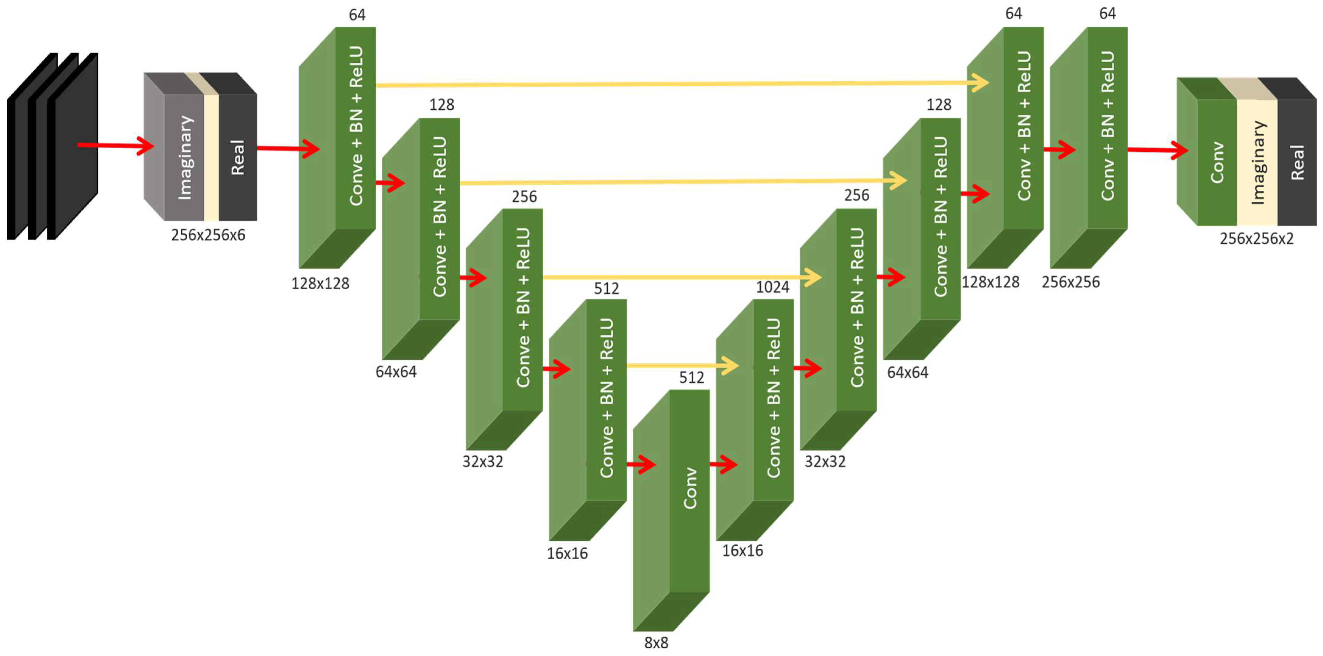
2.2. Model Architecture
3. Results and Discussion
4. Conclusions
Author Contributions
Funding
Informed Consent Statement
Data Availability Statement
Acknowledgments
Conflicts of Interest
References
- Chen, Y.; Schönlieb, C.-B.; Liò, P.; Leiner, T.; Dragotti, P.L.; Wang, G.; Rueckert, D.; Firmin, D.; Yang, G.J. AI-based reconstruction for fast MRI—A systematic review and meta-analysis. Proc. IEEE 2022, 110, 224–245. [Google Scholar] [CrossRef]
- Feng, C.-M.; Yang, Z.; Chen, G.; Xu, Y.; Shao, L. Dual-octave convolution for accelerated parallel MR image reconstruction. In Proceedings of the AAAI Conference on Artificial Intelligence, Vancouver, BC, Canada, 2–9 February 2021; pp. 116–124. [Google Scholar]
- Yang, C.; Liao, X.; Wang, Y.; Zhang, M.; Liu, Q. Virtual Coil Augmentation Technology for MRI via Deep Learning. arXiv 2022, arXiv:2201.07540. [Google Scholar]
- Shan, S.; Gao, Y.; Liu, P.Z.; Whelan, B.; Sun, H.; Dong, B.; Liu, F.; Waddington, D.E.J. Distortion-Corrected Image Reconstruction with Deep Learning on an MRI-Linac. arXiv 2022, arXiv:2205.10993. [Google Scholar]
- Hollingsworth, K.G. Reducing acquisition time in clinical MRI by data undersampling and compressed sensing reconstruction. Phys. Med. Biol. 2015, 60, R297. [Google Scholar] [CrossRef] [PubMed]
- Lee, J.-H.; Kang, J.; Oh, S.-H.; Ye, D.H. Multi-Domain Neumann Network with Sensitivity Maps for Parallel MRI Reconstruction. Sensors 2022, 22, 3943. [Google Scholar] [CrossRef] [PubMed]
- Scott, A.D.; Wylezinska, M.; Birch, M.J.; Miquel, M.E. Speech MRI: Morphology and function. Phys. Med. 2014, 30, 604–618. [Google Scholar] [CrossRef] [PubMed]
- Oostveen, L.J.; Meijer, F.J.; de Lange, F.; Smit, E.J.; Pegge, S.A.; Steens, S.C.; van Amerongen, M.J.; Prokop, M.; Sechopoulos, I. Deep learning-based reconstruction may improve non-contrast cerebral CT imaging compared to other current reconstruction algorithms. Eur. Radiol. 2021, 31, 5498–5506. [Google Scholar] [CrossRef]
- Lebel, R.M. Performance characterization of a novel deep learning-based MR image reconstruction pipeline. arXiv 2020, arXiv:2008.06559. [Google Scholar]
- Lv, J.; Wang, C.; Yang, G.J.D. PIC-GAN: A parallel imaging coupled generative adversarial network for accelerated multi-channel MRI reconstruction. Diagnostics 2021, 11, 61. [Google Scholar] [CrossRef]
- Schlemper, J.; Caballero, J.; Hajnal, J.V.; Price, A.; Rueckert, D. A Deep Cascade of Convolutional Neural Networks for MR image Reconstruction. In Information Processing in Medical Imaging; Springer: Berlin/Heidelberg, Germany, 2017. [Google Scholar]
- Jiang, M.; Yuan, Z.; Yang, X.; Zhang, J.; Gong, Y.; Xia, L.; Li, T. Accelerating CS-MRI reconstruction with fine-tuning Wasserstein generative adversarial network. IEEE Access 2019, 7, 152347–152357. [Google Scholar] [CrossRef]
- Mardani, M.; Gong, E.; Cheng, J.Y.; Vasanawala, S.S.; Zaharchuk, G.; Xing, L.; Pauly, J.M. Deep generative adversarial neural networks for compressive sensing MRI. IEEE Trans. Med. Imaging 2018, 38, 167–179. [Google Scholar] [CrossRef] [PubMed]
- Sandilya, M.; Nirmala, S.; Saikia, N. Compressed Sensing MRI Reconstruction Using Generative Adversarial Network with Rician De-noising. Appl. Magn. Reson. 2021, 52, 1635–1656. [Google Scholar] [CrossRef]
- Wu, Y.; Ma, Y.; Liu, J.; Du, J.; Xing, L. Self-attention convolutional neural network for improved MR image reconstruction. Inf. Sci. 2019, 490, 317–328. [Google Scholar] [CrossRef] [Green Version]
- Rempe, M.; Mentzel, F.; Pomykala, K.L.; Haubold, J.; Nensa, F.; Kröninger, K.; Egger, J.; Kleesiek, J. k-strip: A novel segmentation algorithm in k-space for the application of skull stripping. arXiv 2022, arXiv:2205.09706. [Google Scholar]
- Bydder, M.; Larkman, D.; Hajnal, J. Combination of signals from array coils using image-based estimation of coil sensitivity profiles. Magn. Reson. Med. 2002, 47, 539–548. [Google Scholar] [CrossRef] [PubMed]
- Shitrit, O.; Riklin Raviv, T. Accelerated Magnetic Resonance Imaging by Adversarial Neural Network. In Deep Learning in Medical Image Analysis and Multimodal Learning for Clinical Decision Support; Springer: Berlin/Heidelberg, Germany, 2017; pp. 30–38. [Google Scholar]
- Pruessmann, K.P.; Weiger, M.; Scheidegger, M.B.; Boesiger, P. SENSE: Sensitivity encoding for fast MRI. Magn. Reson. Med. 1999, 42, 952–962. [Google Scholar] [CrossRef]
- HashemizadehKolowri, S.; Chen, R.-R.; Adluru, G.; Dean, D.C.; Wilde, E.A.; Alexander, A.L.; DiBella, E.V. Simultaneous multi-slice image reconstruction using regularized image domain split slice-GRAPPA for diffusion MRI. Med. Image Anal. 2021, 70, 102000. [Google Scholar] [CrossRef]
- Candès, E.J. Compressive sampling. In Proceedings of the International Congress of Mathematicians, Madrid, Spain, 22–30 August 2006. [Google Scholar]
- Liu, B.; Zou, Y.M.; Ying, L. SparseSENSE: Application of compressed sensing in parallel MRI. In Proceedings of the 2008 International Conference on Information Technology and Applications in Biomedicine, Shenzhen, China, 30–31 May 2008. [Google Scholar]
- Wen, B.; Ravishankar, S.; Bresler, Y. Structured overcomplete sparsifying transform learning with convergence guarantees and applications. Int. J. Comput. Vis. 2015, 114, 137–167. [Google Scholar] [CrossRef]
- Qin, C.; Schlemper, J.; Caballero, J.; Price, A.N.; Hajnal, J.V.; Rueckert, D. Convolutional recurrent neural networks for dynamic MR image reconstruction. IEEE Trans. Med. Imaging 2018, 38, 280–290. [Google Scholar] [CrossRef]
- Ruijsink, B.; Puyol-Antón, E.; Usman, M.; van Amerom, J.; Duong, P.; Forte, M.N.V.; Pushparajah, K.; Frigiola, A.; Nordsletten, D.A.; King, A.P.; et al. Semi-automatic Cardiac and Respiratory Gated MRI for Cardiac Assessment during Exercise. In Molecular Imaging, Reconstruction and Analysis of Moving Body Organs, and Stroke Imaging and Treatment; Springer: Berlin/Heidelberg, Germany, 2017; pp. 86–95. [Google Scholar]
- Bhatia, K.K.; Caballero, J.; Price, A.N.; Sun, Y.; Hajnal, J.V.; Rueckert, D. Fast reconstruction of accelerated dynamic MRI using manifold kernel regression. In Proceedings of the International Conference on Medical Image Computing and Computer-Assisted Intervention, Munich, Germany, 5–9 October 2015; pp. 510–518. [Google Scholar]
- Hammernik, K.; Klatzer, T.; Kobler, E.; Recht, M.P.; Sodickson, D.K.; Pock, T.; Knoll, F. Learning a variational network for reconstruction of accelerated MRI data. Magn. Reson. Med. 2018, 79, 3055–3071. [Google Scholar] [CrossRef]
- Aggarwal, H.K.; Mani, M.P.; Jacob, M. MoDL: Model-based deep learning architecture for inverse problems. IEEE Trans. Med. Imaging 2018, 38, 394–405. [Google Scholar] [CrossRef] [PubMed]
- Zhou, Z.; Han, F.; Ghodrati, V.; Gao, Y.; Yin, W.; Yang, Y.; Hu, P. Parallel imaging and convolutional neural network combined fast MR image reconstruction: Applications in low-latency accelerated real-time imaging. Med. Phys. 2019, 46, 3399–3413. [Google Scholar] [CrossRef] [PubMed]
- Du, T.; Zhang, H.; Li, Y.; Pickup, S.; Rosen, M.; Zhou, R.; Song, H.K.; Fan, Y. Adaptive convolutional neural networks for accelerating magnetic resonance imaging via k-space data interpolation. Med. Image Anal. 2021, 72, 102098. [Google Scholar] [CrossRef] [PubMed]
- Schlemper, J.; Qin, C.; Duan, J.; Summers, R.M.; Hammernik, K. Σ-net: Ensembled Iterative Deep Neural Networks for Accelerated Parallel MR Image Reconstruction. arXiv 2019, arXiv:1912.05480. [Google Scholar]
- Lv, J.; Wang, P.; Tong, X.; Wang, C. Parallel imaging with a combination of sensitivity encoding and generative adversarial networks. Quant. Imaging Med. Surg. 2020, 10, 2260. [Google Scholar] [CrossRef]
- Arvinte, M.; Vishwanath, S.; Tewfik, A.H.; Tamir, J.I. Deep J-Sense: Accelerated MRI Reconstruction via Unrolled Alternating Optimization. In Proceedings of the International Conference on Medical Image Computing and Computer-Assisted Intervention, Strasbourg, France, 27 September–1 October 2021. [Google Scholar]
- Souza, R.; Bento, M.; Nogovitsyn, N.; Chung, K.J.; Loos, W.; Lebel, R.M.; Frayne, R. Dual-domain cascade of U-nets for multi-channel magnetic resonance image reconstruction. Magn. Reson. Imaging 2020, 71, 140–153. [Google Scholar] [CrossRef]
- Li, Z.; Sun, N.; Gao, H.; Qin, N.; Li, Z. Adaptive subtraction based on U-Net for removing seismic multiples. IEEE Trans. Geosci. Remote Sens. 2021, 59, 9796–9812. [Google Scholar] [CrossRef]
- Chen, Y.; Firmin, D.; Yang, G. Wavelet improved GAN for MRI reconstruction. In Medical Imaging 2021: Physics of Medical Imaging; SPIE: Bellingham, WA, USA, 2021; Volume 11595, pp. 285–295. [Google Scholar]
- Zhang, K.; Zuo, W.; Gu, S.; Zhang, L. Learning deep CNN denoiser prior for image restoration. In Proceedings of the IEEE Conference on Computer Vision and Pattern Recognition, Honolulu, HI, USA, 21–26 July 2017. [Google Scholar]
- Kulkarni, K.; Lohit, S.; Turaga, P.; Kerviche, R.; Ashok, A. Reconnet: Non-iterative reconstruction of images from compressively sensed measurements. In Proceedings of the IEEE Conference on Computer Vision and Pattern Recognition, Las Vegas, NV, USA, 27–30 June 2016. [Google Scholar]
- Jin, K.H.; McCann, M.T.; Froustey, E.; Unser, M. Deep convolutional neural network for inverse problems in imaging. IEEE Trans. Image Process. 2017, 26, 4509–4522. [Google Scholar] [CrossRef]
- Song, P.; Weizman, L.; Mota, J.F.; Eldar, Y.C.; Rodrigues, M.R.D. Coupled dictionary learning for multi-contrast MRI reconstruction. IEEE Trans. Med. Imaging 2019, 39, 621–633. [Google Scholar] [CrossRef]
- Adler, J.; Öktem, O. Learned primal-dual reconstruction. IEEE Trans. Med. Imaging 2018, 37, 1322–1332. [Google Scholar] [CrossRef]
- Putzky, P.; Welling, M. Recurrent inference machines for solving inverse problems. arXiv 2017, arXiv:1706.04008. [Google Scholar]
- Sajjad, M.; Khan, S.; Muhammad, K.; Wu, W.; Ullah, A.; Baik, S.W. Multi-grade brain tumor classification using deep CNN with extensive data augmentation. J. Comput. Sci. 2019, 30, 174–182. [Google Scholar] [CrossRef]
- Afshar, P.; Mohammadi, A.; Plataniotis, K.N. Brain tumor type classification via capsule networks. In Proceedings of the 2018 25th IEEE International Conference on Image Processing (ICIP), Athens, Greece, 7–10 October 2018. [Google Scholar]
- Zhang, J.; Xie, Y.; Wu, Q.; Xia, Y. Medical image classification using synergic deep learning. Med. Image Anal. 2019, 54, 10–19. [Google Scholar] [CrossRef] [PubMed]
- Isensee, F.; Kickingereder, P.; Wick, W.; Bendszus, M.; Maier-Hein, K.H. Brain tumor segmentation and radiomics survival prediction: Contribution to the brats 2017 challenge. In Proceedings of the International MICCAI Brainlesion Workshop, Quebec City, QC, Canada, 14 September 2017. [Google Scholar]
- Khan, H.; Shah, P.M.; Shah, M.A.; ul Islam, S.; Rodrigues, J.J.P.C. Cascading handcrafted features and Convolutional Neural Network for IoT-enabled brain tumor segmentation. Comput. Commun. 2020, 153, 196–207. [Google Scholar] [CrossRef]
- Han, Y.; Yoo, J.; Kim, H.H.; Shin, H.J.; Sung, K.; Ye, J.C. Deep learning with domain adaptation for accelerated projection-reconstruction MR. Magn. Reson. Med. 2018, 80, 1189–1205. [Google Scholar] [CrossRef] [PubMed]
- Healy, J.J.; Curran, K.M.; Serifovic Trbalic, A. Deep Learning for Magnetic Resonance Images of Gliomas. In Deep Learning for Cancer Diagnosis; Springer: Berlin/Heidelberg, Germany, 2021; pp. 269–300. [Google Scholar]
- Shabbir, A.; Ali, N.; Ahmed, J.; Zafar, B.; Rasheed, A.; Sajid, M.; Ahmed, A.; Dar, S.H. Satellite and scene image classification based on transfer learning and fine tuning of ResNet50. Math. Probl. Eng. 2021, 2021, 5843816. [Google Scholar] [CrossRef]
- Waddington, D.E.; Hindley, N.; Koonjoo, N.; Chiu, C.; Reynolds, T.; Liu, P.Z.; Zhu, B.; Bhutto, D.; Paganelli, C.; Keall, P.J.J.a.p.a. On Real-time Image Reconstruction with Neural Networks for MRI-guided Radiotherapy. arXiv 2022, arXiv:2202.05267. [Google Scholar]
- Guo, P.; Wang, P.; Zhou, J.; Jiang, S.; Patel, V.M. Multi-institutional collaborations for improving deep learning-based magnetic resonance image reconstruction using federated learning. In Proceedings of the IEEE/CVF Conference on Computer Vision and Pattern Recognition, Montreal, QC, Canada, 11–17 October 2021. [Google Scholar]
- Yiasemis, G.; Sonke, J.-J.; Sánchez, C.; Teuwen, J. Recurrent Variational Network: A Deep Learning Inverse Problem Solver applied to the task of Accelerated MRI Reconstruction. In Proceedings of the IEEE/CVF Conference on Computer Vision and Pattern Recognition, New Orleans, LA, USA, 19–24 June 2022. [Google Scholar]


| Sr. No. | Reference | Methodology | Results | Future Directions |
|---|---|---|---|---|
| 1 | [35] | Reconstruction of brain MRI data using a G1M U-Net model | Reconstruction results are derived from practical sampling schemes of accelerated brain MRIs. | Apply to a wide range of datasets with excellent fidelity to fully sample scans. |
| 2 | [36] | Use of a GAN with a Cyclic Loss to Reconstruct a CS-MRI | In terms of both running time and image quality, CS-MRI methods performed noticeably better than open-source MRI datasets. | The next step in the study will be to extend Refine GAN to handle dynamic MRI. |
| 3 | [37] | The inverse problem was solved using a deep CNN-based optimization model. | Discriminative CNN denoiser creates a versatile, quick, and efficient image restoration framework. | _ _ _ _ |
| 4 | [38] | Image Reconstruction from Compressively Sensed Random Measurements Using Recon Net | Recon Net offers high-quality reconstructions of simulated and actual data for various measurement rates. | _ _ _ _ |
| 5 | [39] | To resolve problems with normal-convolutional inverse, direct inversion and a CNN are proposed. | Parallel beam X-ray CT sparse-view network performance is calculated. | It is possible to address strategies for heterogeneous datasets. |
| 6 | [40] | CS-based approaches, especially DLMRI, use a coordinate-descent algorithm to optimize. | CNNs were evaluated for their relevance to the MR image reconstruction challenge. | The model will directly address the coil sensitivity maps’ redundancy. |
| 7 | [41] | The Primal-Dual algorithm for tomographic reconstruction has been learned. | For the Shepp–Logan phantom, they improve peak SNR by 6 dB over competing approaches. | Capable of using complex loss functions with learned reconstruction operators. |
| 8 | [42] | Recurrent Neural Networks are used by RIMs to solve inverse problems. | The RIM-3task model is competitive on all noise levels. | _ _ _ _ |
| 9 | [43] | A pre-trained CNN model was used to augment and classify brain tumor data. | Before and after data augmentation, they outperformed the most sophisticated algorithms with 90.67 accuracies. | Weight-saving CNN fine-grained classification will use differential stochastic classification. |
| 10 | [44] | Investigate the overfitting issue using a CapsNet for classifying brain tumors. | Comparative research with CNN found their accuracy rate was 86.56%. Learning rate decreases with iterations. | In the future, look into how adding more layers affects classification accuracy. |
| 11 | [45] | A review of medical image classification using deep learning approaches. | They explain deep learning algorithms and how they can be used for medical imaging, noting that the learning rate is proportional to the inverse of iterations. | To apply the strategies to the modalities where they are not employed, more research is needed. |
| 12 | [46] | Predicted patient survival using BraTS2017 and U-NET. | With less computational time, 89.6% accuracy was achieved. | _ _ _ _ |
| 13 | [47] | BRaTS 2013, 2015 used CNN-based two-path architecture to separate brain tumors. | Cascaded input CNN achieved 88.2% accuracy. Analysis of various architectural designs. | Increasing the architecture layers and data set boosted the outcomes even more. |
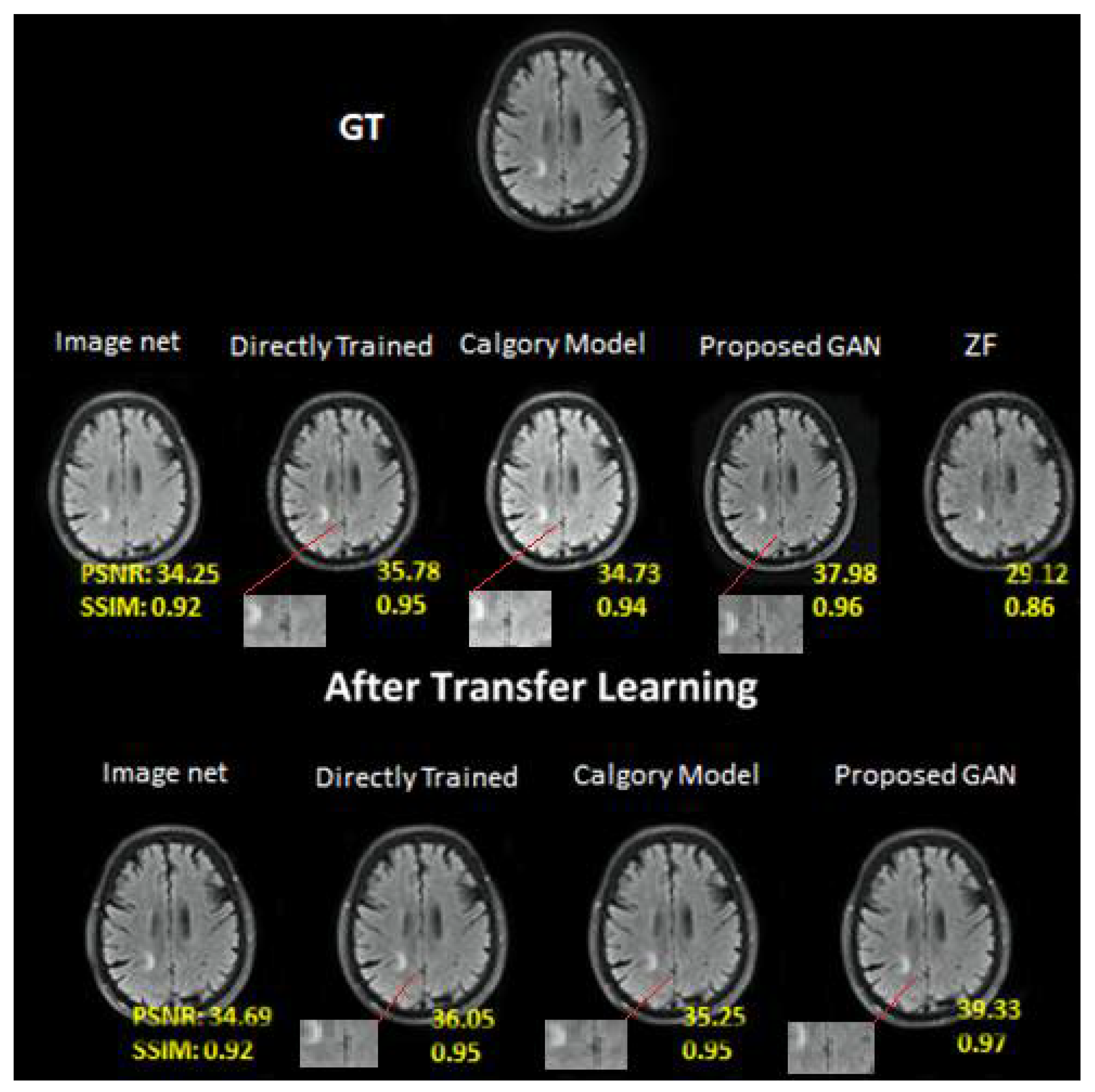
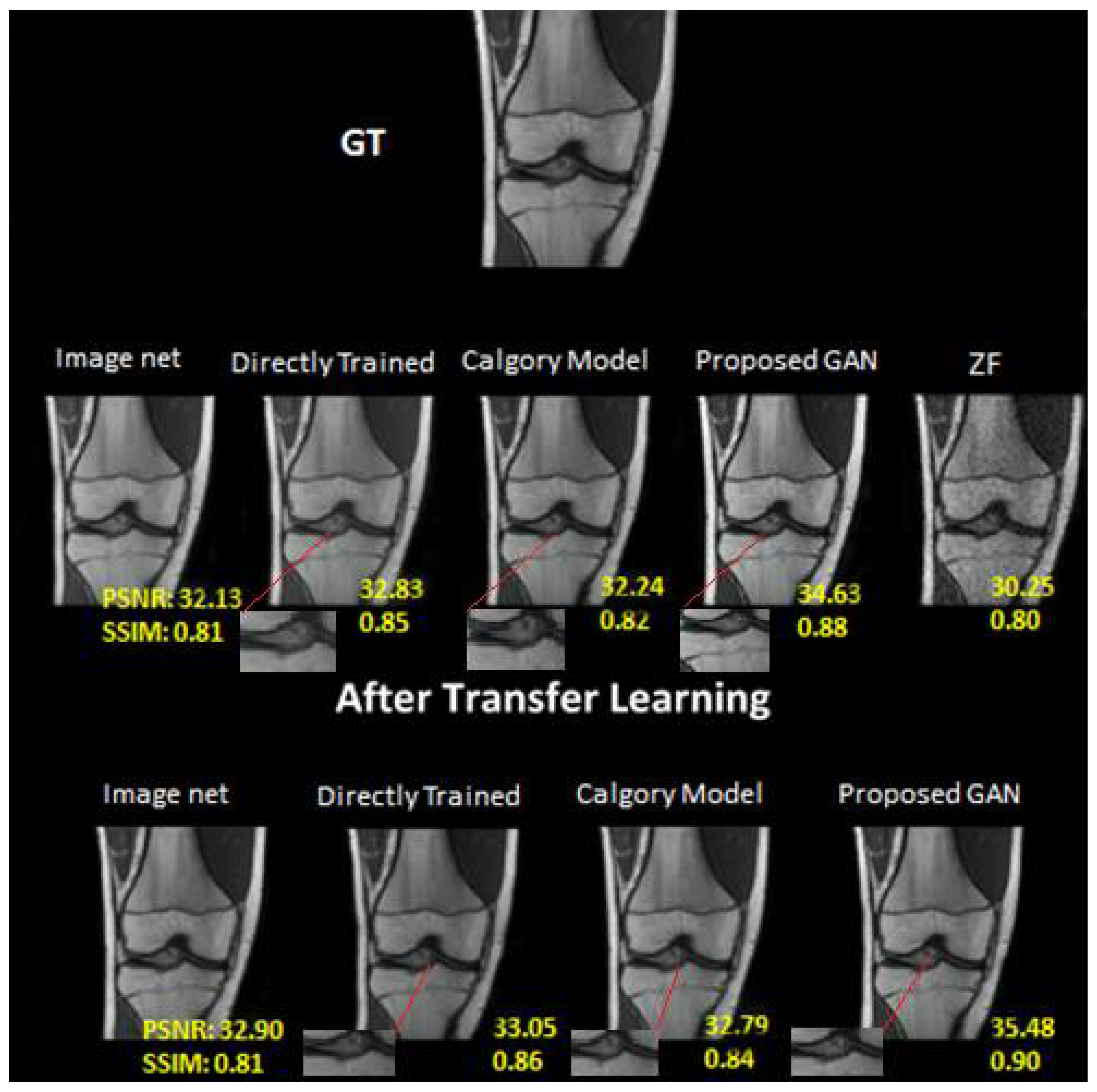
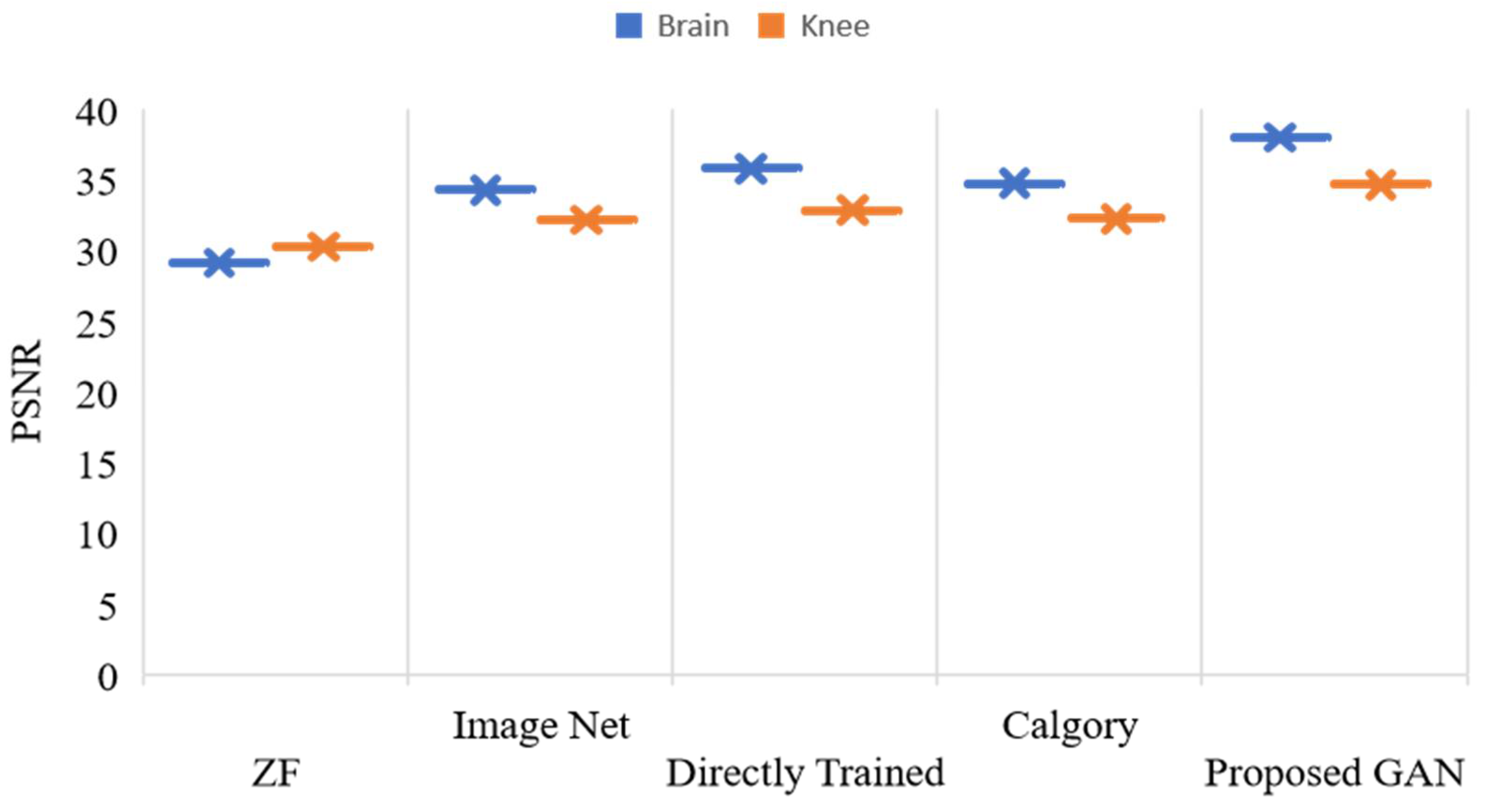
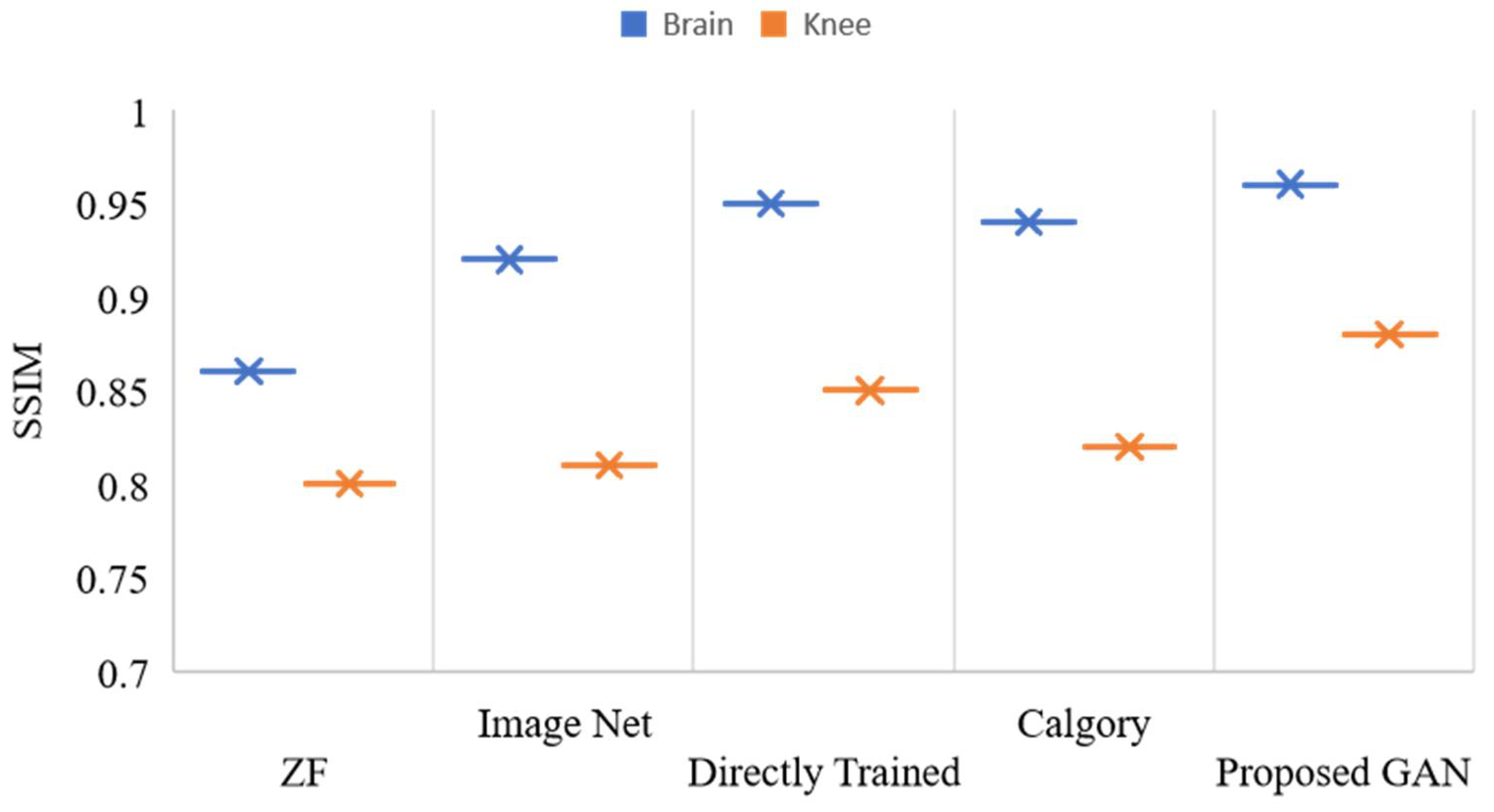
| Brain | Knee | |||
|---|---|---|---|---|
| PSNR | SSIM | PSNR | SSIM | |
| ZF | 29.12 | 0.86 | 30.25 | 0.80 |
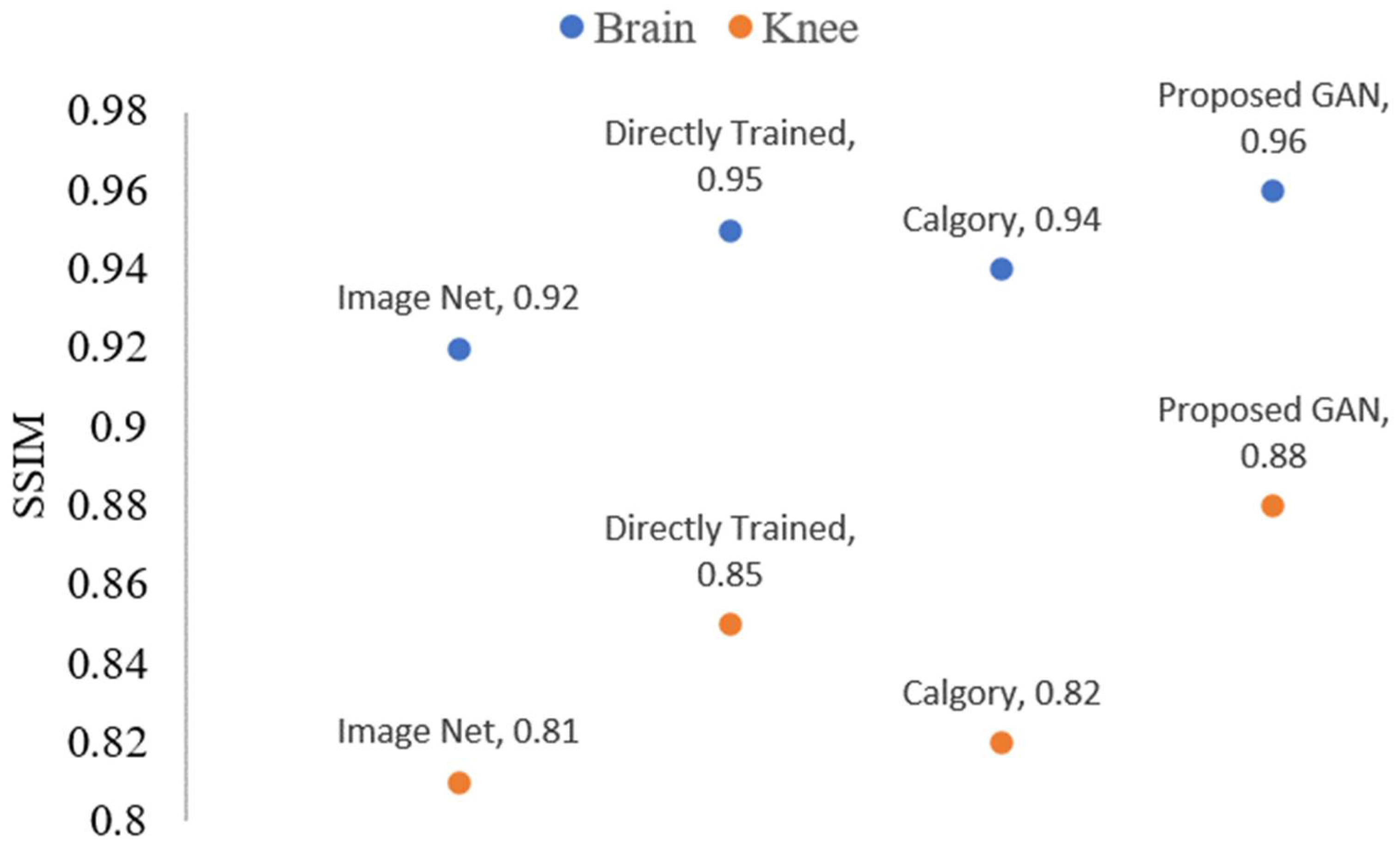
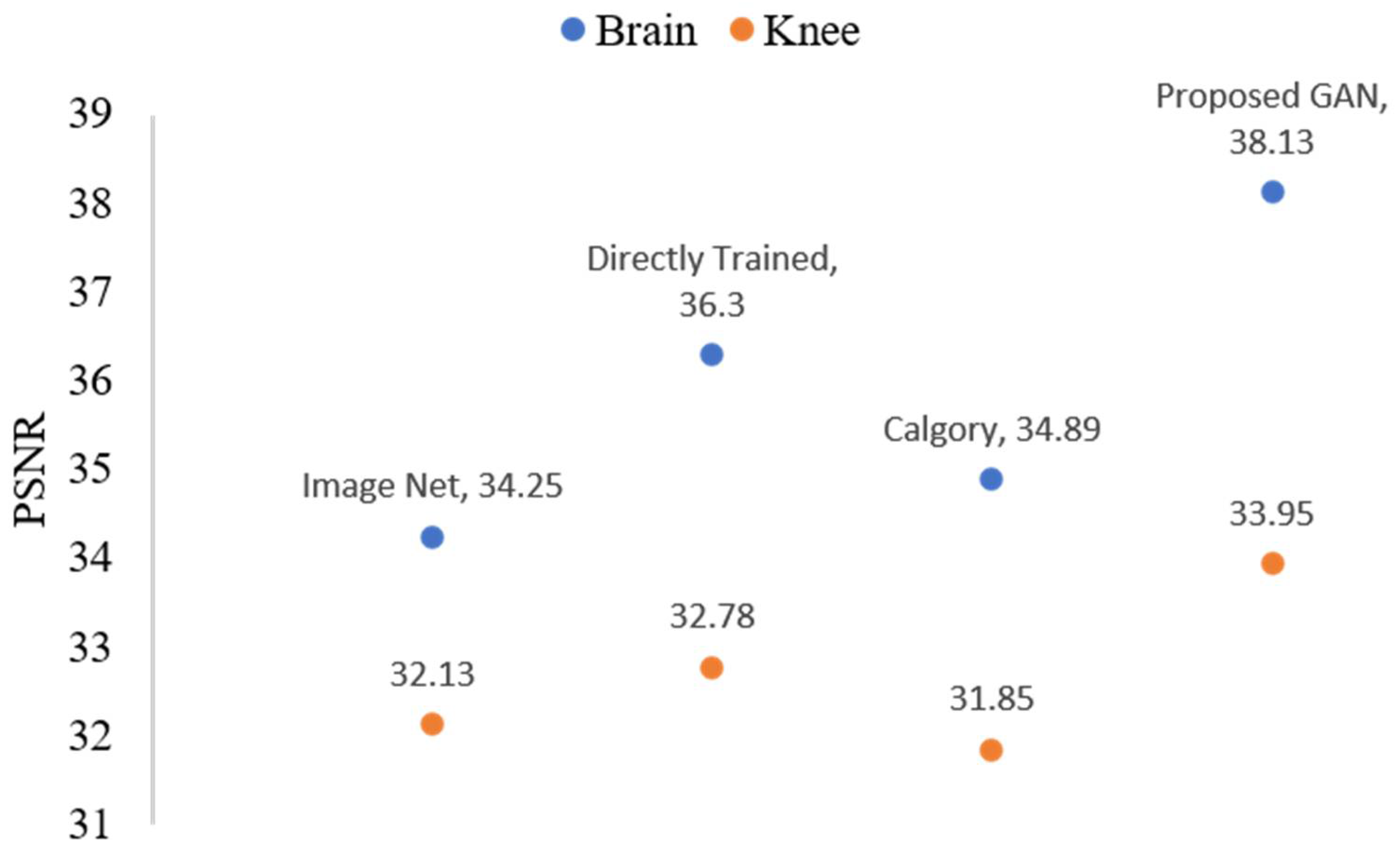
| ImageNet [51] | 34.25 | 0.92 | 32.13 | 0.81 |
| Directly Trained [52] | 35.78 | 0.95 | 32.83 | 0.85 |
| Calgary Model [53] | 34.73 | 0.94 | 32.24 | 0.82 |
| Proposed GAN | 37.98 | 0.96 | 34.63 | 0.88 |
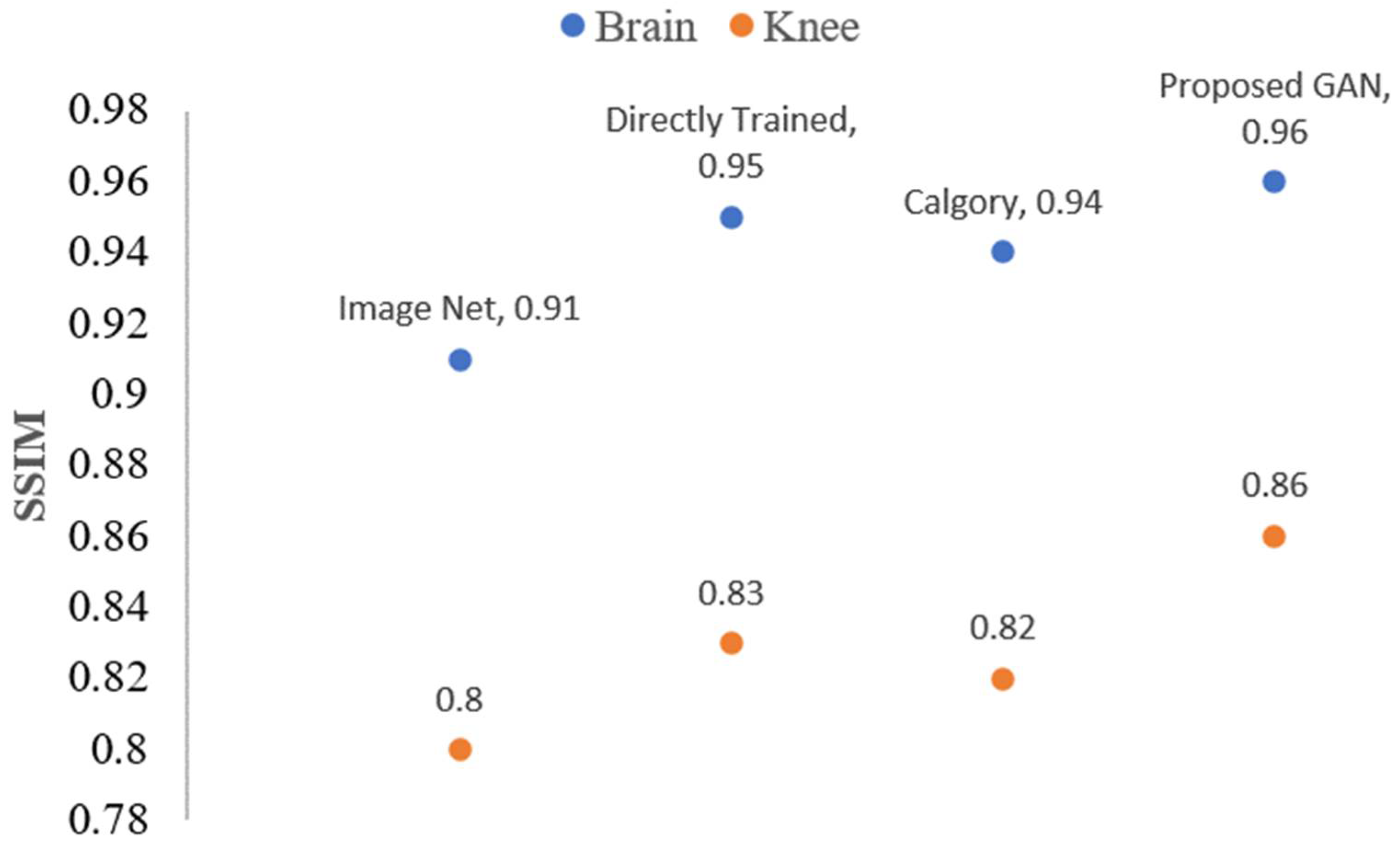
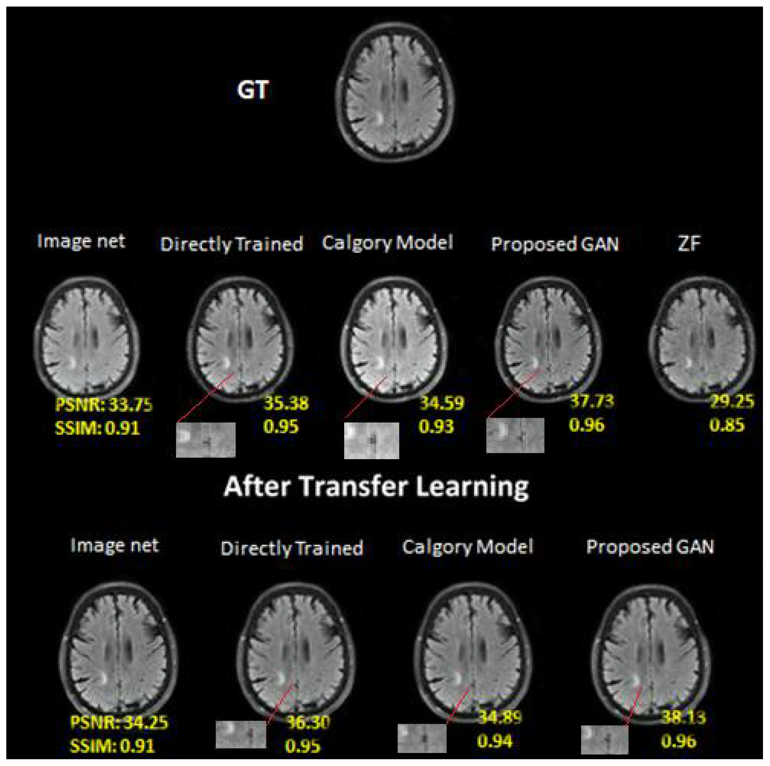
| Brain | Knee | |||
|---|---|---|---|---|
| PSNR | SSIM | PSNR | SSIM | |
| ImageNet [51] | 34.69 | 0.92 | 32.90 | 0.81 |
| Directly Trained [52] | 36.05 | 0.95 | 33.05 | 0.86 |
| Calgary Model [53] | 35.25 | 0.95 | 32.79 | 0.84 |
| Proposed GAN-TL | 39.33 | 0.97 | 35.48 | 0.90 |
Publisher’s Note: MDPI stays neutral with regard to jurisdictional claims in published maps and institutional affiliations. |
© 2022 by the authors. Licensee MDPI, Basel, Switzerland. This article is an open access article distributed under the terms and conditions of the Creative Commons Attribution (CC BY) license (https://creativecommons.org/licenses/by/4.0/).
Share and Cite
Yaqub, M.; Jinchao, F.; Ahmed, S.; Arshid, K.; Bilal, M.A.; Akhter, M.P.; Zia, M.S. GAN-TL: Generative Adversarial Networks with Transfer Learning for MRI Reconstruction. Appl. Sci. 2022, 12, 8841. https://doi.org/10.3390/app12178841
Yaqub M, Jinchao F, Ahmed S, Arshid K, Bilal MA, Akhter MP, Zia MS. GAN-TL: Generative Adversarial Networks with Transfer Learning for MRI Reconstruction. Applied Sciences. 2022; 12(17):8841. https://doi.org/10.3390/app12178841
Chicago/Turabian StyleYaqub, Muhammad, Feng Jinchao, Shahzad Ahmed, Kaleem Arshid, Muhammad Atif Bilal, Muhammad Pervez Akhter, and Muhammad Sultan Zia. 2022. "GAN-TL: Generative Adversarial Networks with Transfer Learning for MRI Reconstruction" Applied Sciences 12, no. 17: 8841. https://doi.org/10.3390/app12178841
APA StyleYaqub, M., Jinchao, F., Ahmed, S., Arshid, K., Bilal, M. A., Akhter, M. P., & Zia, M. S. (2022). GAN-TL: Generative Adversarial Networks with Transfer Learning for MRI Reconstruction. Applied Sciences, 12(17), 8841. https://doi.org/10.3390/app12178841