Article

Mathematical Modeling and Robust Control of a Restricted State Suspended Biped Robot Implementing Linear Actuators for Articulation Mobilization

1
CINVESTAV-IPN, Mexico City 07360, Mexico
2
Tecnologico de Monterrey, Institute of Advanced Materials for Sustainable Manufacturing, Monterrey 64849, Mexico
*
Author to whom correspondence should be addressed.
Appl. Sci. 2022, 12(17), 8831; https://doi.org/10.3390/app12178831
Submission received: 4 July 2022 / Revised: 18 August 2022 / Accepted: 24 August 2022 / Published: 2 September 2022
(This article belongs to the Section Robotics and Automation)

Abstract

:
The aim of this study is to develop an adaptive automatic control method for solving the trajectory tracking problem for a biped robotic device (BRD) and taking into account that each articulation is mobilized by a linear actuator. Each extremity of the BRD has three articulations with a linear actuator enforcing the controlled motion for each articulation. The control problem considers the task of tracking reference trajectories that define a regular gait cycle. The suggested adaptive control form has state-dependent gains that drive the tracking error into an invariant and attractive ellipsoidal with a center at the origin; meanwhile, the articulation restrictions are satisfied permanently. The stability analysis based on a controlled Lyapunov function depending on the tracking error leads to the explicit design of the state-dependent adaptive gains. Taking into account the forward complete setting of the proposed BRD, an output feedback formulation of the given adaptive controller is also developed using a finite-time and robust convergent differentiator based on the super-twisting algorithm. A virtual dynamic representation of the BRD is used to test the proposed controller using a distributed implementation of the adaptive controller. Numerical simulations corroborate the convergence of the tracking error, while all the articulation restrictions are satisfied using the adaptive gains. With the purpose of characterizing the proposed controller, a sub-optimal tuned regular state feedback controller is used as a comparative approach for validating the suggested design. Among the compared controllers, the analysis of the convergence of the mean square error of the tracking error motivates the application of the designed adaptive variant.

1. Introduction

The development of BRDs has attained a significant degree of maturity over the last three decades. Novel advances in mechanical design, electrical instrumentation, and automatic control methods have forced BRDs to exert more complex activities such as autonomous walking, climbing stairs, and jumping, among others [1]. Nowadays, there is a scientific and technical trend in developing more efficient BRD configuration, which includes using lighter and more resistant materials, faster digital processors, and more advanced electronic sensors and actuators [2]. This last aspect has attracted attention because actuators’ characteristics define most BRD mobilization abilities. There are diverse actuator options for BRDs, including permanent magnet and brushless motors, steppers, pneumatic muscles [3], multi-motor drive systems [4], and more recently, linear actuators [5].
Linear actuators are devices that are conformed by an electrical motor (usually a DC with a permanent magnet) connected to a ball-screw driving structure (
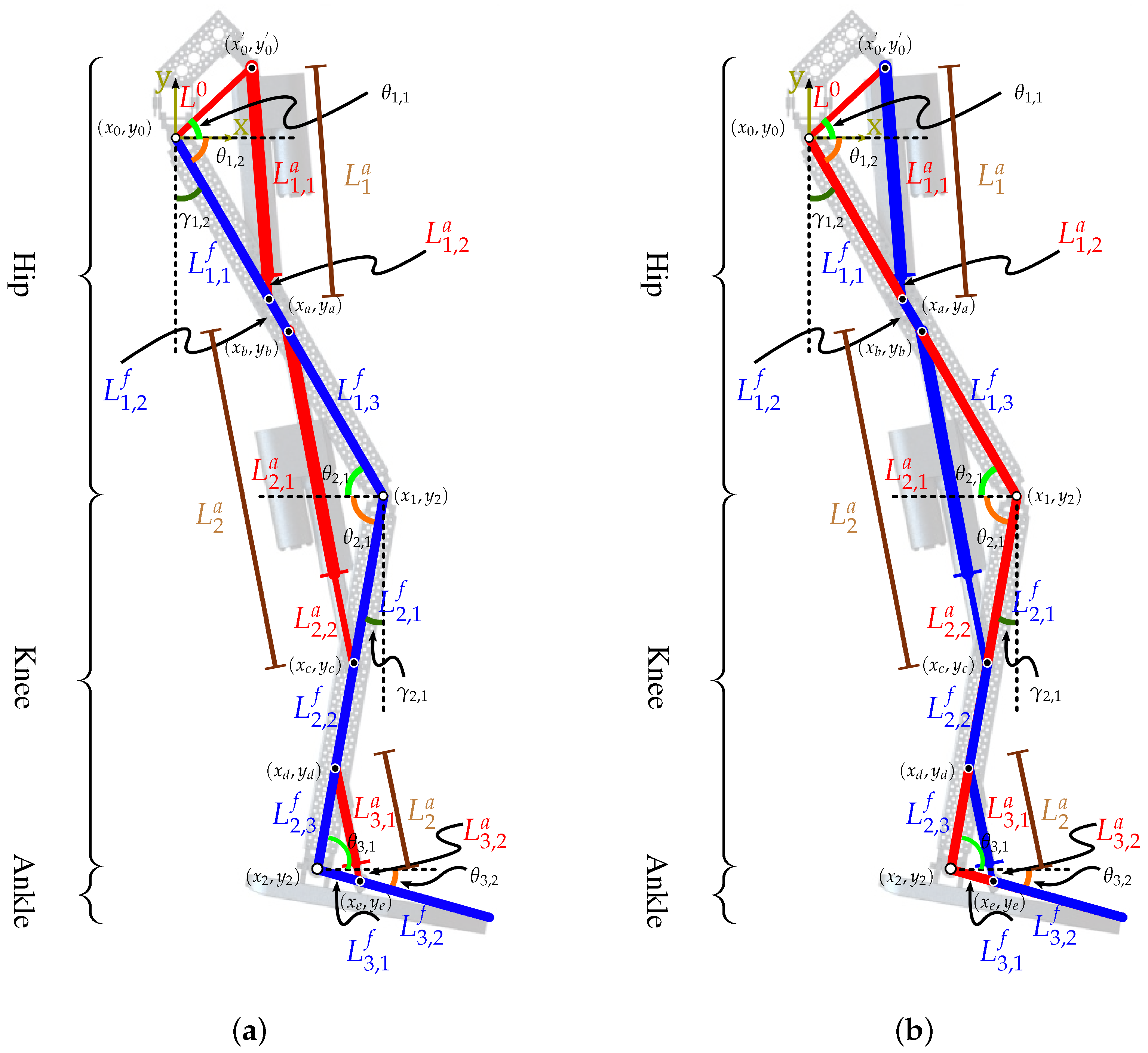
Figure 1). This device is used increasingly in robotics due to its working characteristics, including the device scalability, setup versatility, stack setting, larger torque, the electrical equivalent operation similar to DC motors actuators, and motion robustness concerning external perturbations, as well as long periods of activity. Using linear actuators for mobilizing BRD has several advantages (compared to other actuation strategies). A heavy actuation device can be placed near the hip joint, limiting the leg inertia, and some others [6]. Despite the mentioned benefits, some drawbacks must be overcome if the linear actuators are going to be considered a feasible variant for forcing the BRDs motion. Among others, linear actuator dynamics are usually not considered in the device modeling description. The restricted range of motion in the actuator (which implies limited articulation angular displacement) are the main disadvantages that should be corrected.
All the benefits of using linear actuators as driving elements for BRDs have been emphasized by various studies. The Technical University of Munich constructed the humanoid robot LOLA [7]. They proposed the design of a linear actuator based on a ball screw drive attached to the main structure by Cardan joints. It is used to maintain the moment of inertia of the thigh. Furthermore, the WL family of robots, designed by Waseda University, uses linear motion actuators for its Stewart platform-like mechanism that is oriented as a novel biped walking type wheelchair [8,9]. The study introduced in [10] describes a double linear ball-screw drive structure for the ankle joint. In comparison, ref. [11] provides a design where both the knee and ankle possess single and double linear actuator structures, respectively.
Most existing studies where the linear actuator has been the active driving element of biped robots have not considered the electromechanical dynamics that characterize it. Such dynamics include the motor’s temporal evolution and connection to the ball-screw configuration. Moreover, the reported studies consider that the linear actuator has an unbounded range of linear displacement. Both characteristics are going to be analyzed in this study and used as limitations for the automatic control design that may enforce the exerting of a gait cycle (even if the BRD is suspended).
The problem of introducing linear actuator dynamics in the BRD augments the complexity not only of its mathematical model but also of the automatic control design that forces the regulated movement of the BRD [12]. In addition, the linear actuator attached to the BRD also introduces a mechanical reconfiguration in the BRD because of the actuator’s mechanical structure, which is now giving up a new mass distribution [13], forcing new damping and restricting the angular displacement at each articulation of the BRD (Figure 1). Including linear actuators in BRD electromechanical configurations introduces novel challenges for the automatic control design. Despite the development of automatic controllers for BRD that has been studied for a long time, the dynamical nature of linear actuators implies some new design paradigms, where the actuator now plays a mechanical role as well as exerting the driving force to the BRD [14,15].
The characteristics of linear actuators force an increase in the number of states in the actuated BRD and bound the control action considering the limited velocity of the linear actuator and the restricted screw movement range. These particular settings must be considered in the control design requirements for BRD, which are adjoined to the presence of modeling imprecision and external uncertainties. All these challenging aspects can be overcome if the proposed control design is robust but, at the same time, can satisfy the successful tracking of the designed reference trajectories that define the needed articulation movements for the BRD. Most of the reported control designs for BRD have not considered such restrictions. Furthermore, many studies have not considered BRD designs’ movement restrictions at each joint. Hence, an imprecise gain tuning process for the controllers aimed to mobilize each of the joints, and the robot may manifest unwanted effects in the curse of the transient period. These reasons have motivated the design of automatic controllers that may consider all the referred states or/and control limitations. Penalty state-dependent function, convex set projections, composite state convex sets, and adaptive gain barrier Lyapunov function have been considered the most preferable options to assess the effect of state restrictions on the control design.
Barrier Lyapunov function (BLF) is considered a preferable option that could be related to restricted articulation movement. The number of applications of BLF has grown in recent years due to the benefits of restricted systems’ transient and steady operation. Diverse classes of BLF have been around since the beginning of the previous century, considering the logarithmic, integral, and tangent variants, just to list some of them.
Robotic devices with biped configurations controlled by adaptive gains defined by the application of BLF have shown significant benefits over systems using traditional control formulations such as state feedback, extended state approaches, sliding modes, and many others. However, there is a growing number of applications using adaptive state-dependent gains for the proposed controllers, which are calculated using controlled BLF. However, no reported study proposes the application of adaptive controllers based on BLF for linear actuators for BRDs.
This study introduces a novel design for a state-dependent adaptive controller for a BRD, including the presence of linear actuators in the robot configuration. The control design considers state restrictions in the linear actuator and all the BRD articulations while tracking reference trajectories corresponding to developing a regulated gait cycle for a BRD. The study also includes the dynamics of the DC motor that drives the linear actuator motion.
The central objective of this study is to present the development of an adaptive automatic control method to resolve the trajectory tracking control design related to a BRD that considers that each articulation is driven by a regular electrical linear actuator. As a consequence, the main contributions of this study are the following: (a) the development of an adaptive state-dependent controller, which is estimated with the application of a controlled BLF; (b) the formal stability proof, which yields the calculus of gains depending on the states, which ensure the solution of the reference tracking for the BRD, including the linear actuator dynamics and (c) the numerical evaluations, considering the application of a virtual BRD yield to confirm the effectiveness of the proposed controller.
This manuscript is organized according to the following strategy. The modeling strategy presented in Section 2 details the method to include the linear actuator presence for each articulation in the BRD. This section also shows the mathematical model of the BRD, including the dynamics of the linear actuators driving the movement of each articulation in the robot. Section 3 describes the proposed adaptive controller based on the application of logarithmic BLF functions and its corresponding proof and a variant of the proposed controller implementing the estimation of the tracking error via a set of super-twisting robust differentiators. Section 4 details the virtual BpR designed to test the proposed controller implemented in Sim-Mechanics/Matlab. The numerical evaluations of the controller are presented in Section 5, where the proposed controller is compared with a classical PID controller. Finally, in Section 6, the conclusions of this paper are presented.

2. Mathematical Modeling Strategy

Including linear actuators on the biped robot structure introduces two possible modeling strategies. The first one considers the passive mechanical structure as the core part to be modeled and the linear actuators as the active section that provides the mobilization of the mechanical parts. The second strategy includes using the linear actuator as part of the mechanical structure. The difference between these strategies can be visualized considering the mechanical and active sections shown in Figure 1.
This section presents the general characteristics of the modeling strategies. For both models, this study considers the following characteristics:
  • The biped robot can mobilize the legs on the sagittal plane,
  • The contact points between the actuator tip and the structural section of the biped are not dynamic. Then, there is no dynamic contact (stiffness-damping).
  • The linear actuator for each articulation is a lead screw and nut structure, which is developing the linear action related to the linear actuator.
  • The actuator is activated by a DC motor, which is also considered part of the control design.
  • All articulations in the biped robot are static based on a rotational joint which is justified using the argument related to the motion in the sagittal plane.
  • The biped robot is suspended, and it does not have any impact contact with the supporting surface. These kinds of robots are aimed to serve as a basis for exoskeleton devices, which can contribute to the rehabilitation processes.
Considering that q Q R n is the vector of generalized coordinates and q ˙ Q R n , then the kinetic energy T : Q × Q R + , T = T q , q ˙ and the potential energy U : Q R + , U = U ( q ) for the complete system may be obtained from the aggregated analysis of subsystems forming the biped robot. The energetic components of the individual subsystems can be calculated independently. Hence, the equations of motion are obtained with the calculation of the Euler–Lagrange equations:
d d t q ˙ i L q , q ˙ q i L q , q ˙ = τ i Ξ i
Here, we present the generalized forcing–dissipation terms τ i R , Ξ i R , and the Lagrangian: L q , q ˙ = T ( q , q ˙ ) U ( q ) . The principles justifying this formalism can be consulted in classical mechanics textbooks. Except for the differentiation that may become cumbersome for systems with many articulations, the Euler–Lagrange equations formalism can be applied straightforwardly because it is based on energetic-based functions. Based on the calculus for the Lagrangian and the application of the Euler–Lagrange schemes, the complete model for a single leg of the BRD satisfies the following differential equation:
M q ( t ) d 2 d t 2 q ( t ) + C d d t q ( t ) , q ( t ) d d t q ( t ) + G q ( t ) = τ ( t ) Ξ ( t )
where q Q R 3 is the vector of angular positions that includes all joints of a single leg in the exoskeleton. The inertia matrix is represented by M : R 3 R 3 × 3 , C : R 3 × R 3 R 3 × 3 is the matrix of Coriolis and centrifugal forces, G : R 3 R 3 includes the terms related to the gravitational forces. The time-dependent term Ξ R 3 is the vector that represents the effect of viscous and dried frictions, external perturbations and modeling imprecision.

2.1. Development of Mathematical Model 1

The mechanical section of the biped robot depicted in Figure 1a is made up of fixed links that are interconnected by the linear actuator structures. This figure demonstrates the configuration of the articulations in the BRD, which are restricted by the linear movement of the actuator.
The expression of the kinetic energy of this first model corresponds to
T = k = 1 3 T m k f θ 1 , 2 , θ 2 , 2 , θ 3 , 2 , θ ˙ 1 , 2 , θ ˙ 2 , 2 , θ ˙ 3 , 2 + k = 1 3 T m k , 1 a γ 1 , γ 2 , γ 3 , γ ˙ 1 , γ ˙ 2 , γ ˙ 3 + k = 1 3 T m k , 2 a γ 1 , γ 2 , γ 3 , γ ˙ 1 , γ ˙ 2 , γ ˙ 3
where the individual kinetic energies for the masses in the biped robot are presented below. The first section of individual kinetic energies corresponds to the masses of the fixed mechanical sections of the BRD (solid links), i.e., T m 1 f , T m 2 f and T m 3 f , respectively, for the three sections of the device:
T m 1 f = 1 2 m 1 f 0.5 L 1 f 2 θ ˙ 1 , 2 2
T m 2 f = 1 2 m 2 f L 1 f 2 θ ˙ 1 , 2 2 + 1 2 m 2 f L 2 f 2 2 θ ˙ 2 , 2 2 m 2 f L 1 f L 2 f c o s θ 1 , 2 θ 2 , 2 θ ˙ 1 , 2 θ ˙ 2 , 2
T m 3 f = 1 2 m 3 f L 1 f 2 θ ˙ 1 , 2 2 + 1 2 m 3 f L 2 f 2 θ ˙ 2 , 2 2 + 1 2 m 3 f L 3 f 2 2 θ ˙ 3 , 2 2 2 m 3 f L 1 f L 2 f c o s θ 1 , 2 θ 2 , 2 θ ˙ 1 , 2 θ ˙ 2 , 2 + m 3 f L 1 f L 3 f c o s θ 1 , 2 θ 3 , 2 θ ˙ 1 , 2 θ ˙ 3 , 2 m 3 f L 2 f L 3 f c o s θ 2 , 2 θ 3 , 2 θ ˙ 2 , 2 θ ˙ 3 , 2
The second section of individual kinetic energies corresponds to the fixed mechanical sections of each linear actuator in the BRD, i.e., T m j , 1 a , j = 1 , 2 , 3 , respectively, for the three actuators of the device:
T m j , 1 a = T m j , 1 a r + 1 4 m j , 1 a L j , 1 a 2 γ ˙ j 2 + m j , 1 a L j , 1 a x ˙ j , 1 a , r c o s γ j y ˙ j , 1 a , r s i n γ j
where T m j , 1 a r is
T m j , 1 a r = 1 2 m j , 1 a x ˙ j , 1 a , r 2 + y ˙ j , 1 a , r 2
The third section of individual kinetic energies corresponds to the mobile mechanical sections of each linear actuator in the BRD, i.e., T m j , 2 a , j = 1 , 2 , 3 , respectively, for the three actuators of the device:
T m j , 2 a = T m j , 2 a r + 1 4 m j , 2 a L j , 1 a 2 γ ˙ j 2 + 1 8 m j , 2 a L ˙ j , 2 a 2 + 1 8 m j , 2 a L j , 2 a 2 γ ˙ j 2 + m j , 2 a L j , 1 a x ˙ j , 1 a , r c o s γ j y ˙ j , 1 a , r s i n γ j + 1 2 m j , 2 a L ˙ j , 2 a x ˙ j , 1 a , r s i n γ j + y ˙ j , 1 a , r c o s γ j + 1 2 m j , 2 a L j , 2 a γ ˙ j x ˙ j , 1 a , r c o s γ j y ˙ j , 1 a , r s i n γ j + 1 2 m j , 2 a L j , 1 a L ˙ j , 2 a s i n ( γ j γ j ) + 1 2 m j , 2 a L j , 1 a L j , 2 a c o s ( 2 γ j ) + 1 4 m j , 2 a L j , 2 a L ˙ j , 2 a s i n ( γ j γ j ) γ ˙ j
where T m j , 2 a r corresponds to
T m j , 2 a r = 1 2 m j , 2 a x ˙ j , 2 a , r 2 + y ˙ j , 2 a , r 2
Correspondingly, the formal expression of the potential energy is defined as follows
V = k = 1 3 V m k f θ 1 , 2 , θ 2 , 2 , θ 3 , 2 + k = 1 3 V m k , 1 a γ 1 , γ 2 , γ 3 + k = 1 3 V m k , 2 a γ 1 , γ 2 , γ 3
The first section of individual potential energies corresponds to the masses of the fixed mechanical sections of the BRD (solid links), i.e., V m k f , respectively, for the three sections of the device:
V m k f = m k f g y k f
The second section of individual potential energies corresponds to the fixed mechanical sections of each linear actuator in the BRD, that is, V m j , 1 a , j = 1 , 2 , 3 , respectively, for the three actuators of the device:
V m j , 1 a = m j , 1 a g y j a a
The third section of individual potential energies corresponds to the mobile mechanical sections of each linear actuator in the BRD, that is, V m j , 2 a , j = 1 , 2 , 3 , respectively, for the three actuators of the device:
V m j , 2 a = m j , 2 a g y j b a
The calculus of both the potential and kinetic energies in the BRD uses the estimation of the centers of masses of the fixed sections in the robot x j f and y j f that correspond to
x 1 f = 1 2 L 1 f c o s θ 1 , 2 y 1 f = 1 2 L 1 f s i n θ 1 , 2
x 2 f = L 1 f c o s θ 1 , 2 1 2 L 2 f c o s θ 2 , 2 y 2 f = L 1 f s i n θ 1 , 2 1 2 L 2 f s i n θ 2 , 2
x 3 f = L 1 f c o s θ 1 , 2 L 2 f c o s θ 2 , 2 + 1 2 L 3 f c o s θ 3 , 2 y 3 f = L 1 f s i n θ 1 , 2 L 2 f s i n θ 2 , 2 + 1 2 L 3 f s i n θ 3 , 2
The configuration of the linear actuators in the form shown in Figure 1 implies the necessity of connecting the active length of the actuators with respect to the angular motion obtained at each articulation in the legs of the BRD. These relationships are the following:
L 1 , 1 f 2 = L 0 2 + L 1 a 2 2 L 0 L 1 a c o s γ 1 c L 2 , 1 f 2 = L 1 , 3 f 2 + L 2 a 2 2 L 1 , 3 f L 2 a c o s γ 2 c L 3 , 1 f 2 = L 2 , 3 f 2 + L 3 a 2 2 L 2 , 3 f L 3 a c o s γ 3 c
Complementarily, the angles γ j = π / 2 γ j c with j = 1 , 2 , 3 .
The corresponding coordinates for the fixed sections of the linear actuators are x j a a , y j a a while the coordinates for the mobile section are defined by x j b a , y j b a , which can be expressed as follows
x j a a = x j , 1 a , r + 1 2 L j , 1 a s i n γ j x j b a = x j , 1 a , r + L j , 1 a s i n γ j + 1 2 L j , 2 a s i n γ j y j a a = y j , 1 a , r + 1 2 L j , 1 a c o s γ j y j b a = y j , 1 a , r + L j , 1 a c o s γ j + 1 2 L j , 2 a c o s γ j
where x 1 , 1 a , r = x 0 , y 1 , 1 a , r = y 0 ; x 2 , 1 a , r = x b , y 2 , 1 a , r = y b and x 3 , 1 a , r = x d , y 3 , 1 a , r = y d . The relationships for the coordinates of the fixed and mobile sections require the analysis of the connections between the lengths of the actuators and the angular motions, which are
L 0 2 = x 0 2 + y 0 2 L 1 , 1 f + L 1 , 2 f 2 = x b 2 + y b 2 L 1 f 2 + L 1 f L 2 , 1 f + L 2 , 2 f c o s θ 1 , 2 θ 2 , 2 + 1 4 L 2 , 1 f + L 2 , 2 f 2 = x d 2 + y d 2
The corresponding velocities for the fixed sections of the links in the BRD are the following:
x ˙ 1 f = 1 2 L 1 f s i n θ 1 , 2 θ ˙ 1 , 2 y ˙ 1 f = 1 2 L 1 f c o s θ 1 , 2 θ ˙ 1 , 2
x ˙ 2 f = L 1 f s i n θ 1 , 2 θ ˙ 1 , 2 + 1 2 L 2 f s i n θ 2 , 2 θ ˙ 2 , 2 y ˙ 2 f = L 1 f c o s θ 1 , 2 θ ˙ 1 , 2 1 2 L 2 f c o s θ 2 , 2 θ ˙ 2 , 2
x ˙ 3 f = L 1 f s i n θ 1 , 2 θ ˙ 1 , 2 + L 2 f s i n θ 2 , 2 θ ˙ 2 , 2 1 2 L 3 f s i n θ 3 , 2 θ ˙ 3 , 2 y ˙ 3 f = L 1 f c o s θ 1 , 2 θ ˙ 1 , 2 L 2 f c o s θ 2 , 2 θ ˙ 1 , 2 + 1 2 L 3 f c o s θ 3 , 2 θ ˙ 3 , 2
The corresponding velocities of fixed and mobile masses for the linear actuators are given by
x ˙ j a a = x ˙ j , 1 a , r + 1 2 L j , 1 a c o s γ j γ ˙ j x ˙ j b a = x ˙ j , 1 a , r + L j , 1 a c o s γ j γ ˙ j + 1 2 L ˙ j , 2 a s i n γ j + 1 2 L j , 2 a c o s γ j γ ˙ j y ˙ j a a = y ˙ j , 1 a , r 1 2 L j , 1 a s i n γ j γ ˙ j y ˙ j b a = y ˙ j , 1 a , r L j , 1 a s i n γ j γ ˙ j + 1 2 L ˙ j , 2 a c o s γ j 1 2 L j , 2 a s i n γ j γ ˙ j
Considering the basis of the linear actuators, the following restrictions hold for the relationships between the time-varying lengths of the linear actuators:
x ˙ 1 , 1 a , r 2 + y ˙ 1 , 1 a , r 2 = 0 x ˙ 2 , 1 a , r 2 + y ˙ 2 , 1 a , r 2 = L 1 , 1 f + L 1 , 2 f 2 θ ˙ 1 , 2 2 x ˙ 3 , 1 a , r 2 + y ˙ 3 , 1 a , r 2 = L 1 f 2 θ ˙ 1 , 2 2 + L 2 , 1 f + L 2 , 2 f 2 θ ˙ 2 , 2 2 2 L 1 f L 2 , 1 f + L 2 , 2 f c o s θ 1 , 2 θ 2 , 2 θ ˙ 1 , 2
The mathematical expressions of the linear positions and their corresponding velocities are obtained using the configurations in the BRD and considering the relative motions of all the linear actuator devices with respect to the fixed sections of the BRD.

2.1.1. Tendon-Driven Actuation Principle

The expected behavior of the linear screw-lead and nut device as a linear actuator on the biped robot can be described in the following form: first, an electrical DC motor transfers the rotational motion to a ball screw where the nut is locked in rotation. This configuration allows free space for displacement along the screw axis, using an anti-rotation mechanism. This configuration has been used in diverse linear actuators. This study considered a similar structure. The generated linear displacement of the nut is transmitted over a specific link, which is eventually driving the rotational joint by the associated rotational torque. This configuration permits a single actuation architecture that reproduces tendon routing, therefore reducing friction. Notice that the friction effect associated with the force transmission tendons is the major source of friction in complex mechanical biped robot configurations. In the case of the BRD considered in this study, the activity of the linear actuator operates at the level of rotational torque that mobilizes each articulation. Noticing that each articulation is driven by two main forces (the linear actuator and gravitational), the following relation is considered:
τ i = r i , m i a d 2 d t 2 x s j = 1 N i a r C M , j , m j g
where r i is the vector from the articulated joint and the point of actuator insertion on the robot link, m i a is the mass of the mobile section in the linear actuator, x s is the displacement of the same mobile section, N i a is the number of links placed below the analyzed joint, which induces torque action, r C M , j is the vector connecting the coordinates of the joint and those of the center of mass of each link J, m J is the mass of the link and g is the gravity vector.

2.1.2. Actuator Dynamics

An electromechanical actuator (EMA) is made of an electric DC motor (that corresponds to the electrical section) and an associated mechanical gearbox (that defines the mechanical section). EMAs are categorized in both rotative and linear stages. A linear actuator is as follows: geared and direct-driven linearly operated EMA. The geared linear electromechanical actuator generally consists of a DC motor with a lead-screw (or ball-screw or roller-screw) and a nut assembly. The motor shaft connects to the lead screw using a shaft coupling or a transformation gearbox. The DC motor transforms the electrical energy to the respective rotational motion of the shaft. Hence, the lead screw converts the rotary motion into proportional linear motion. The motor shaft rotates either anti-clockwise or clockwise, depending on the voltage input polarity. Once the rotational motion is transferred to the lead screw, the nut assembles the needed motion (XN), either forward or backward, depending on the forced rotational direction of the shaft.
In the direct-driven linear actuator (considering both electrical and mechanical sections), the nut is the rotational element, and the lead screw represents the translational element. The lead screw structure is accommodated inside the actuator itself, considering the technical composition of the DC motor. The interiorly threaded nut is placed inside the rotor. The rotor and the nut rotate when the engine receives electrical energy. This rotational motion of the nut forces the linear lead-screw motion. The shaft attached to the ending section of the lead screw has slotted grooves. This configuration restricts the rotational motion of the associated lead screw simultaneously with the nut. In terms of their functionalities, the two mentioned actuators are not significantly different. Nonetheless, the direct-driven EMA has a compact size compared to the geared EMA. This configuration makes the direct-driven EMA a suitable and appropriate technical option for aerospace, robotics, and other industries.
Modeling a single EMA is crucial for developing a multi-element set of actuators operating as HRA. This section presents the mathematical model of a direct-driven linear EMA. The electric circuit implies that the supplied electrical power using a given voltage ( V a ) forces the current i a flow whose conduction is opposed by the conducting path resistance ( R a ) , inductance ( L a ) and a back electromechanical force or e.m.f. for short ( V b ) , which is equivalent to K e d θ m d t . The voltage balance is expressed as:
K e d d t θ m + L a d d t i a + R a i a = V a
Here K e represents the back e.m.f parameter. The parameter θ m characterizes the angular variation of the DC motor. In the mechanical part, inertia, damping, and frictional settings are concentrated parameters. When the electromagnetic torque performed by the electrical section is supplied to the mechanical section of the actuator (lead-screw and nut) rotational element, it moves at a given rate of d d t θ m , which corresponds to the given moment of inertia J m . The angular speed of both sections, the rotor and the nut are the same because they are attached to each other [13].
The variables labeled as x s and x l represent linear variations of the lead screw and the load correspondingly. The matrix K s defines the relative stiffness existing between the lead screw with respect to the nut. The damping between the bearing and rotor is defined by the variable C s . The produced torque τ m is operating in opposition by damping torque τ d , load torque τ l and the inertial torque τ i . Therefore, the electromagnetic-related torque is balanced by the other three developed torques [16], that is:
τ m = τ d + τ l + τ i τ m = K t i a τ d = D d d t θ m τ i = J d 2 d t 2 θ m τ l = C s · l 2 π x ˙ s x ˙ l + K s · l 2 π x s x l
where D is viscous damping at the armature. The torque τ m produced as a function of the current i a that passes through the armature appears in (28). The matrix K t defines the torque constant. Equivalently, the inertial, damping, and load torques are described in the subsequent expressions in (28), respectively. In that equation, the term l 2 π is used for converting the angular displacement of the nut to linear displacement of the lead screw, where l is the screw lead. The substitution of τ m , τ d , τ l and τ i in (28) and bringing the electrical relationship in (27) yields:
K t i a = D d d t θ m + C s · l 2 π x ˙ s x ˙ l + K s · l 2 π x s x l + J d 2 d t 2 θ m K e d d t θ m + R a i a + L a d d t i a = V a
with x s = ( l · θ ) / ( 2 · π ) the relationship between the angular displacement and the displacement of the linear actuator (considering the lead screw configuration). In terms of the movement efficiency, the following relationship is also valid d d t x s = Γ r d d t θ 1 η · τ i , where Γ r is the resistive torque, and η is the ball-screw efficiency.
The application of the assumption describing the class of interaction between the tip of the actuator and the link in the biped robot results in x s = x l . Using the state variable theory for each actuator τ i with the definitions χ 1 , i A = θ m , i , χ 2 , i A = θ ˙ m , i and χ 3 , i A = i a , i and the corresponding parameters (labeled with a superscript i) yields the following model for the actuator:
d d t χ 1 , i A = χ 2 , i A d d t χ 2 , i A = D i J i χ 2 , i A + K t , i J i χ 3 , i A d d t χ 3 , i A = K e , i L a , i χ 2 , i A R a , i L a , i χ 3 , i A + V a , i L a , i
The pushing force of the linear actuator can be estimated as F i A = m i A d d t χ 2 , i A , therefore the torque τ i = L i , 1 f · F i A · s i n ( δ i ) produced by this force over the joint i corresponds to δ i = π θ m , i γ i c .

2.2. Development of Mathematical Model 2

Considering that the actuators are considered part of the mechanical section of the biped robot, let us consider the model presented in Figure 1. This section develops the geometrical analysis that integrates the mechanical section and the actuator’s dynamic movement. Considering the model in Figure 1 and studying the section corresponding to the hip section, the following relations are valid:
θ 1 = θ 1 , 1 + θ 1 , 2
The fixed relation between ( x 0 , y 0 ) and ( x 0 , y 0 ) yields
θ 1 , 1 = a t a n y 0 y 0 x 0 x 0
Now consider that the length of the selected linear actuator for the hip section L 1 a is given by L 1 a = L 1 , 1 a + L 1 , 2 a . In view of the mechanical relation between ( x 0 , y 0 ) , ( x 0 , y 0 ) and ( x a , y a ) , the following equation is produced:
L 1 a 2 = L 0 2 + L 1 , 1 f 2 2 L 0 L 1 , 1 f c o s θ 1
In view of (33), γ 1 , 2 = 0.5 π θ 1 , 2 , the following relations are valid:
c o s γ 1 , 2 = y 0 y a L 1 , 1 f = y 0 y b L 1 , 1 f + L 1 , 2 f = y 0 y 1 L 1 f s i n γ 1 , 2 = x 0 x a L 1 , 1 f = x 0 x b L 1 , 1 f + L 1 , 2 f = x 0 x 1 L 1 f
Using a similar geometrical study for the knee study, the following angular equation is valid:
θ 2 = θ 2 , 1 + θ 2 , 2
The static relation given for ( x b , y b ) and ( x 1 , y 1 ) yields
θ 2 , 1 = a t a n y b y 1 x b x 1
Taking into account the length of the selected linear actuator for the knee section, L 2 a is given by L 2 a = L 2 , 1 a + L 2 , 2 a . In view of the mechanical relation between ( x b , y b ) , ( x 1 , y 1 ) and ( x c , y c ) , the following equation is produced:
L 2 a 2 = L 1 , 3 f 2 + L 2 , 1 f 2 2 L 1 , 3 f L 2 , 1 f c o s θ 2
In view of (37), γ 2 , 2 = 0.5 π θ 2 , 2 , the following relations are valid:
c o s γ 2 , 2 = y 1 y c L 2 , 1 f = y 1 y d L 2 , 1 f + L 2 , 2 f = y 1 y 2 L 2 f s i n γ 2 , 2 = x 1 x c L 2 , 1 f = x 1 x d L 2 , 1 f + L 2 , 2 f = x 1 x 2 L 2 f
For the ankle analysis, the corresponding angular equation is valid:
θ 3 = θ 3 , 1 + θ 3 , 2
The static relation given for ( x d , y d ) and ( x 2 , y 2 ) yields
θ 3 , 1 = a t a n y d y 2 x d x 2
In view of the length of the selected linear actuator for the ankle section, L 3 a corresponds to L 3 a = L 3 , 1 a + L 3 , 2 a . Considering the mechanical relation between ( x d , y d ) , ( x 2 , y 2 ) and ( x e , y e ) yields:
L 3 a 2 = L 2 , 3 f 2 + L 3 , 1 f 2 2 L 2 , 3 f L 3 , 1 f c o s θ 3
According to (41), γ 3 , 2 = 0.5 π θ 3 , 2 , the following relations are valid:
c o s γ 3 , 2 = x 2 x e L 3 , 1 f = x 2 x 3 L 3 f s i n γ 3 , 2 = y 2 y e L 3 , 1 f = y 2 y 3 L 3 f
According to the mechanical relations described in this section, the kinetic and potential energies can be obtained in the form presented in the Mathematical Model 1. The calculus is omitted just to avoid unnecessary repetition of similar information.
Notice that integrating the actuator as an active element of the mechanical section simplifies the analysis of the actuator effect. Indeed, one may notice that mathematical modeling of the actuator dynamics for this case corresponds to τ m in (28), with τ d = τ l = 0 . Therefore, the model for the actuation system inside the actuator (which is operating here as a prismatic joint) satisfies the dynamics presented in (30) with D i = 0 .
Despite that this second model appears as a more simple version of the mathematical description of the BRD, it could be more complicated to use in the control design formulation.

3. Automatic Control of Biped Robot with Linear Actuators

This section demonstrates how to implement linear actuators as part of the biped robot structure. The modeling strategy considers two options,

3.1. Control Realization for Biped Robot Using Linear Ball Screwdrivers as Actuation Devices

The dynamic model of a single leg presented in (2) can be represented (with ζ α : = q and ζ β : = d d t q ) as follows [17,18]:
d d t ζ α ( t ) = ζ β ( t ) d d t ζ β ( t ) = f ζ ( t ) , t + g ζ α ( t ) τ ( t ) + Υ ζ ( t ) , t y ( t ) = ζ α ( t )
with ζ = [ ζ α , ζ β ] , where ζ X R 2 n , X is an open subspace of the state space, ζ α R n is a vector formed with the angles describing the angular motions related to each joint in the BRD. The vector ζ β R n represents the derivative of the angular motions for each joint with respect to time. The variable y represents the available output information that can be measured from the biped robot. The vector filed f : X × R + R n defines the internal dynamics of the BRD. The structure of this function can be obtained using the Euler–Lagrange method. This study does not study the interactions between contacting surface and the BRD. The mathematical properties of the field f guarantee the local Lipschitz condition given here:
f ζ 1 f ζ 2 L f ζ 1 ζ 2 , ζ 1 X , ζ 2 X , L f R +
The matrix g : R n R n × n defines how the input action modifies the dynamics of the BRD. The structure of this matrix corresponds to the inverse of the inertia matrix for the BRD, which is positive definite. This matrix satisfies the following inequality (45) uniformly on t 0 (using the Frobenius matrix norm):
0 < g g ζ α F g + < + g R + , g + R +
The term Υ : X × R + R n represents the uncertainties/perturbations, and it belongs to the following set:
Ξ = Υ | sup t 0 , ζ R n Υ 2 Υ 0 + Υ 1 ζ 2
Because of the nature of the mechanical structure, it must satisfy the angular displacement restrictions for all the components of the state vector:
< ζ α , i ζ α , i ζ α , i + < + , ζ α , i , ζ α , i + R
This study assumes that an upper limit exists ζ + , given as follows:
( max i ζ i + ) n λ m i n P = ζ +
where ζ i characterizes the motion restriction for the ith angular displacement and P R n × n is a positive definite weighting matrix. Such a matrix may be used to impose some specific articulation restrictions. Therefore, ζ + provides the bounds for the BRD states according to the following relationship:
ζ P 2 ζ +
The term Υ corresponds to Υ = M 1 Ξ . A biped robot actuated with linear ball screwdrivers gains postural force. Usually, an individual driver is placed at each articulation forming the configuration observed in Figure 1.

3.2. Output Feedback Control of Biped Robot

This section details all the elements in the automatic control design, including the implementation of the output feedback form, the implementation strategy as well as a brief sketch of the stability proof for the close loop dynamics.
The aim of this study is to develop an output feedback control u = u ( t ) for a biped robot such that
ζ a ( t ) ζ a * ( t ) β 0 , t T > 0
Here, T is a given time, and the positive scalar β 0 defines the quality of the tracking trajectory for the reference trajectory ζ a * , which satisfies the following ordinary differential equation:
d d t ζ α * ( t ) = ζ β * ( t ) d d t ζ β * ( t ) = h ζ α * ( t ) , ζ β * ( t ) , t
Here the vector field h : X × X × R + R n is a locally Lipschitz function, which characterizes the reference trajectories. The reference trajectories are proposed to satisfy the same bounds that are admitted for the angular displacements of each joint, that is
< ζ α , i ζ α , i * ζ α , i + < + , ζ α , i , ζ α , i + R
Defining the trajectory tracking error δ ( t ) R 2 n , which is given by δ = ζ ζ * , where ζ * = [ ( ζ α * ) , ( ζ β * ) ] . Hence, the dynamics of δ ( t ) are given by:
d d t δ ( t ) = A δ ( t ) + B f ζ ( t ) , t + g ζ α ( t ) τ ( t ) + B Υ ζ ( t ) , t h ζ α * ( t ) , ζ β * ( t ) , t A = 0 n I n 0 n 0 n B = 0 n I n
The matrices A and B satisfy a companion controllable form with the correct dimensions.
The controller design considered in this study assumes that the control form satisfies the following linear form with a state-dependent gain
τ ( t ) = g 1 ( ζ a ( t ) ) K ( t ) δ ^ ( t ) h ζ α * ( t ) , ζ β * ( t ) , t f ζ ( t ) , t
Notice that this formulation appears to be a class of adaptive state-dependent feedback for the class of biped robot. In the controller form, δ ^ is the tracking error using the estimates of ζ β . The gain of the suggested controller is defined as K ( t ) = K P ( t ) K D ( t ) with K P R n × n and K D R n × n .
The linear control form has well-known efficient tracking characteristics, and its implementation requires measuring d d t y t . The possibility of obtaining the estimation of such derivatives online usually implies important technical resources such as additional sensors. A feasible alternative is instrumenting a class of RED, which can yield an accurate estimation of the time derivative of d d t y t [19]. This study uses the significant benefits of the STA method, which has proven to be one of the more efficient alternatives to obtain an accurate estimation of the time derivative of the output information, while it can be used as part of output feedback control forms [20].
For a scalar variable, the STA operating as a RED can be detailed as follows. Consider that w 1 t = r t , with r ( t ) R being the signal that must be differentiated, and w 2 ( t ) = d d t r ( t ) describes its time-derivative. Assuming that d 2 d t 2 r ( t ) r + , it is feasible to propose the following auxiliary dynamic representation
d d t w 1 ( t ) = w 2 ( t ) , d d t w 2 ( t ) = d 2 d t 2 r ( t )
The set of differential equations (55) consists of the state-space description for r ( t ) . The STA used to obtain the derivative of r t satisfies
d d t w ¯ 1 t = w ¯ 2 t λ 1 w ˜ 1 ( t ) 1 / 2 sign w ˜ 1 ( t ) d d t w ¯ 2 t = λ 2 sign w ˜ 1 ( t ) w ˜ 1 = w ¯ 1 w 1 ; d ( t ) = d d t w ¯ 1 t
where w ¯ 1 and w ¯ 2 are the STA variables and λ 1 , λ 2 > 0 are its gains [19]. The time-dependent signal, d ( t ) , represents the output of the RED in (56). Here,
sign ( ν ) = 1 i f ν > 0 [ 1 , 1 ] i f ν = 0 1 i f ν < 0

3.3. Adaptive Output-Feedback Controller including the Joint Restrictions and Actuator Dynamics

The dynamics of each articulation in system (43) can be presented as the composition of n-subsystems as follows:
d d t ζ α , i ( t ) = ζ β , i ( t ) d d t ζ β , i ( t ) = f i ζ ( t ) , t + g i , i ζ α ( t ) τ i ( t ) + j = 1 , j i n g i , j ζ α ( t ) τ j ( t ) + Υ i ζ ( t ) , t τ i ( t ) = L i , 1 f · m i A d d t χ 2 , i A · s i n π χ 1 , i A γ i c d d t χ 1 , i A = χ 2 , i A d d t χ 2 , i A = D i J i χ 2 , i A + K t , i J i χ 3 , i A d d t χ 3 , i A = K e , i L a , i χ 2 , i A R a , i L a , i χ 3 , i A + V a , i L a , i
where ζ a , i and ζ b , i are the i t h and ( n + i ) t h states of (43). The nonlinear forms f i · and g i , i ( · ) are the functions corresponding to the states ζ a , i as well as ζ b , i . Additionally, γ i · , · describes the corresponding uncertain section of the studied subsystem. The positioning of the linear actuator and the movement dynamics of each articulation in the biped robot (43) presented in Figure 1 establishes a relationship between torques at the analyzed i-th joint. This fact is represented in (58).
Based on the definition for the tracking error introduced in (53), the individual tracking error for each angular joint in the biped robot satisfies:
d d t δ i ( t ) = δ i + n ( t ) d d t δ i + n ( t ) = f i ζ ( t ) , t + g i , i ζ α ( t ) τ i ( t ) h i ζ a * ( t ) , ζ b * ( t ) + j = 1 , j i n g i , j ζ α ( t ) τ j ( t ) + Υ i ζ ( t ) , t
Here, the Lipschitz function h i ζ a * ( t ) , ζ b * ( t ) is the i t h component of h ζ a * ( t ) , ζ b * ( t ) . Notice that each tracking error δ i admits the following bounds
δ i : = ζ α , i ζ α , i + < δ i < ζ α , i + ζ α , i = : δ i +
Based on the restrictions estimated for each δ i , the application of asymmetric output-based BLF yields the construction of the proposed controller that drives the corresponding tracking error towards the invariant zone near the origin.
The convergence for the trajectory tracking error δ in (59) can be justified by the arguments described in the next theorem:
Theorem 1.
Consider the BRD system (43), with the control law proposed in (54) and the gains adjusted as in
d d t K P , i t = λ P , i P 1 , i δ i | δ i | α i K P , i t K P , i * d d t K D , i t = λ P , i P 1 , i d d t δ ^ i | δ i | α i K D , i t K D , i *
where δ ^ i is the estimated derivative of δ i . Hence, the controller uses the time-derivative of the tracking error obtained by the implementation of the STA as RED given in (56). If there are positive constants α i , λ 1 , i , λ 2 , i , then the Lyapunov inequalities have positive-definite solutions P 1 , i matrices:
A 1 , i P 1 , i + P 1 , i A 1 , i Q 1 , i A 1 , i = λ 1 , i 1 2 λ 2 , i 0 , Q 1 , i = Q 1 , i > 0 , Q 1 , i R 2 × 2
and if there are positive gains K P , i * , K D , i * that can be selected in such a way that the Riccati equations described by
P 2 , i A 2 , i + α i I + A 2 , i + α i I P 2 , i + P 2 , i R 2 , i P 2 , i + Q 2 , i 0
have positive definite P 2 , i matrices as solutions with
A 2 , i = 0 1 K P , i * K D , i * , R 2 , i = Λ a , i + Λ b , i Q 2 , i = 4 λ max Λ b , i 1 I 2 × 2 + Λ ¯ a , i , Λ ¯ a , i = L i Λ a , i , L i R + Λ a , i = Λ a , i > 0 , Λ b , i = Λ b , i > 0 Λ a , i , Λ b , i R 2 × 2 α i R +
hence, δ = δ 1 , , δ n , δ n + 1 , , δ 2 n is globally ultimately bounded with the ultimate bound given by
lim ¯ t E t P 2 E t i = 1 n γ i α i
where
P 2 = P 2 , 1 0 2 × 2 0 2 × 2 0 2 × 2 P 2 , 2 0 2 × 2 0 2 × 2 0 2 × 2 P 2 , n
and γ i = 2 λ max Λ b , i 1 Υ 0 .
The proof of this theorem is presented at the end of this manuscript.

3.4. Actuator Dynamics and Voltage Determination

In view of the relationships presented for the linear actuator and the control actions obtained in the main theorem of this study,
τ i = L i , 1 f · F i A · s i n ( δ i ) = L i , 1 f · m i A d d t χ 2 , i A · s i n ( δ i ) = L i , 1 f · m i A D i J i χ 2 , i A + K t , i J i χ 3 , i A · s i n ( δ i )
Using the STA, one may substitute χ 2 , i A by its estimate χ ^ 2 , i A , and then the proposed controller may be represented as follows:
τ ^ i = L i , 1 f · m i A D i J i χ ^ 2 , i A + K t , i J i χ 3 , i A · s i n ( δ i )
To obtain the requested voltage in the linear actuator, let us introduce the difference between the needed torque Δ τ i = τ i * τ ^ i , which satisfies the following dynamics
d d t Δ τ i = d d t τ i * d d t L i , 1 f · m i A D i J i χ ^ 2 , i A + K t , i J i χ 3 , i A · s i n ( δ i )
The estimation of the derivative applied in the equation d d t Δ τ i yields the following representation:
d d t Δ τ i = d d t τ i * L i , 1 f · m i A D i J i d d t χ ^ 2 , i A + K t , i J i d d t χ 3 , i A · s i n ( δ i ) + L i , 1 f · m i A D i J i χ ^ 2 , i A + K t , i J i χ 3 , i A · c o s ( δ i ) d d t δ i
The expression given in (70) can be alternatively expressed as follows d d t Δ τ i = Φ i A ( t ) + Γ i A ( t ) V a , i ( t ) , where the expressions for Φ i A ( t ) and Γ i A ( t ) are given here
Φ i A ( t ) = d d t τ i + L i , 1 f m i A J i K t , i K e , i D i J i L a , i sin δ + L i , 1 f m i A D i J i cos δ d d t δ χ ^ 2 , i A + L i , 1 f m i A K t , i R a , i J i D i K t , i J i L a , i sin δ + L i , 1 f m i A K t , i J i cos δ d d t δ χ 3 , i A
and
Γ i A ( t ) = L i , 1 f m i A K t , i J i L a , i sin δ
Thus, the dynamic evolution of the error can be written as:
d d t Δ τ i = F i A δ , χ 2 , i A ^ , χ 3 , i A , t + G i A δ , t V a , i
A potential solution to V a , i ( t ) is
V a , i ( t ) = Γ i A ( t ) 1 k i a s i g n Δ τ i + F i A δ , χ 2 , i A ^ , χ 3 , i A , t
Notice that it is straightforward to prove that the proposed voltage is enforcing the finite-time reproduction of the needed torque for controlling the proposed BRD.

4. Virtualize Finite Time Convergence of the Biped Robot

The evaluation of the proposed controller for the considered BRD with linear actuators was conducted using a virtual representation of the device as well as the linear actuators. The designed representation of the robot, which was originally developed in the SolidWorks® Computer Assisted Design software served to test the proposed differentiator as well as the controller. The design was made considering parameters that agree with actual materials such as aluminum. All the elements in the BRD were designed considering the actual dimensions of an adult of 1.85 m height. The adaptive controller proposed in this study was evaluated using the MATLAB® software using the Simulink® environment with its SimMechanics Toolbox®. The simulation algorithm was developed with the following settings: numeric integration with the fixed step of 10 μs seconds using the Runge–Kutta solver. The control algorithm was developed on a personal computer with a Core I7 processor, 32 GB of RAM memory, no additional graphic processing unit, and running Windows 10 as an operating system.
The evaluation of the developed controller considers a comparison with the classical Proportional-Integral-Derivative (PID) controller. This selection considers the compensation ability for external perturbations that this extended state feedback control form has. The parameters of this controller are modified using the self-tuning algorithm for the PID formulation proposed in Matlab. This algorithm performs a frequency-response estimation experiment, injects signals into the system to be controlled, and measures the output. The method also considers the resulting calculated frequency response for tuning the given PID gains for the controlled system. The application of such a tuning algorithm permits a fair comparison with the developed controller, which is considered the main contribution of this study. When some other parameters produce lesser mean square values for the tracking errors, they may increase the power connected to the controller’s application. The evaluation of the trajectory tracking results considers only a single lower limb, showing the benefits of the controller application.

5. Numerical Evaluations

Figure 2 depicts the numerical results related to the tracking result for the reference trajectory for the left-hip articulation of the BRD using the selected PID and the adaptive controllers. These results confirm that both controllers show similar tracking outcomes. A high-quality tracking of the reference trajectories is attained after 0.2 s for both controllers. The equivalence in the tracking is no longer valid, considering that the proposed adaptive controller tracks the reference without exhibiting fast oscillations as the regular PID enforces. PID cannot provide an efficient, robust tracking of the references, highlighting the suggested controller’s benefits. The three articulations validate this fact on the left side of the biped robot. Consequently, the tracking error converges to a characterized invariant set, which characterizes this study’s main result. Figure 2a–c detail the evolution of angular displacements for the hip, knee and ankle, respectively, including the comparison of PID and the proposed adaptive controller. These individual comparisons confirm that the adaptive controller tracks each reference with smaller oscillations around the reference trajectories.
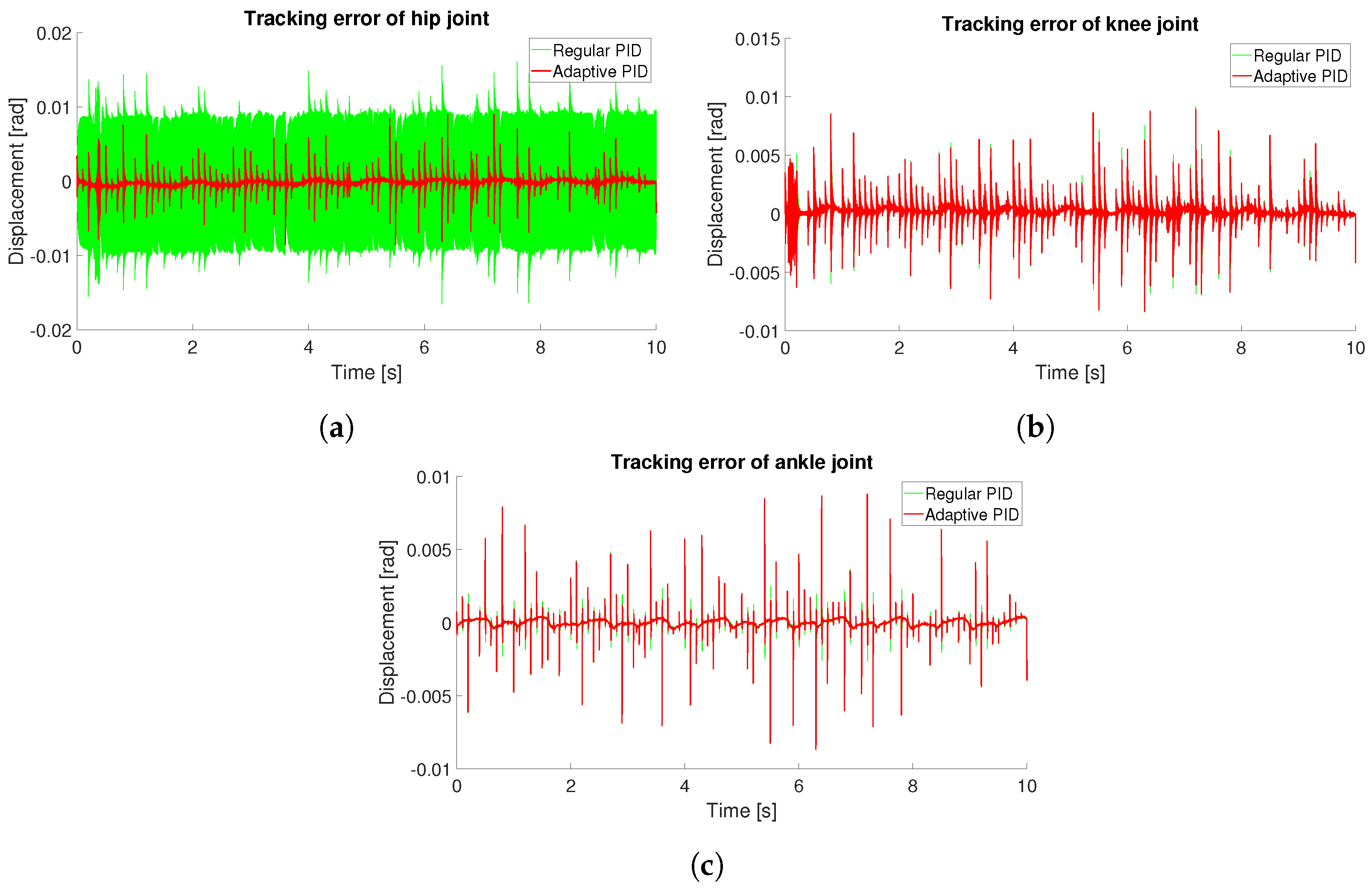
Figure 3 depicts the evolution of the tracking deviations generated with the adaptive and the regular PID controllers. The comparison validates that the selected PID controller produces oscillations with larger amplitudes around the zero value when the time increases. These oscillations confirm that despite the fact that the PID controller may work robustly concerning external perturbations and uncertain modeling sections, there is no efficient tracking of the reference (measured in terms of the tracking errors). At the same time, implementing the adaptive gains improves the tracking quality. Even when the differences between the tracking errors produced by the PID and the adaptive controller are insignificant, their values are relevant in the BDR performing the gait cycle process.
Figure 4 shows the temporal evolution of the Euclidean norm for the tracking deviation produced with the implementation of both controllers, the PID, and the proposed adaptive form. These norms are presented simultaneously here to evaluate the adaptive control quality. The comparison highlights that the suggested controller drives the tracking error toward the origin, implementing both adaptive and PID forms. The more significant norm produced by the PID controller also proves that the adaptive form induces better tracking of the reference trajectory, which yields a better gait cycle developed by the suggested biped robotic device. This figure also shows that the adaptive control form produces a minor mean square error, significantly improving traditional control forms such as the PID.
Figure 5 and Figure 6 compare the torque evolution measured at all three joints in a particular leg of the biped robot. This comparison exhibits similar temporal evolutions for both controllers (for both PID and adaptive structures) for the three articulations. The individual torque obtained for each articulation is larger if the PID controller is compared with the adaptive form. Notice that such comparison confirms that the adaptive form enhances the tracking in both senses, the better tracking quality and the corresponding smaller energy (
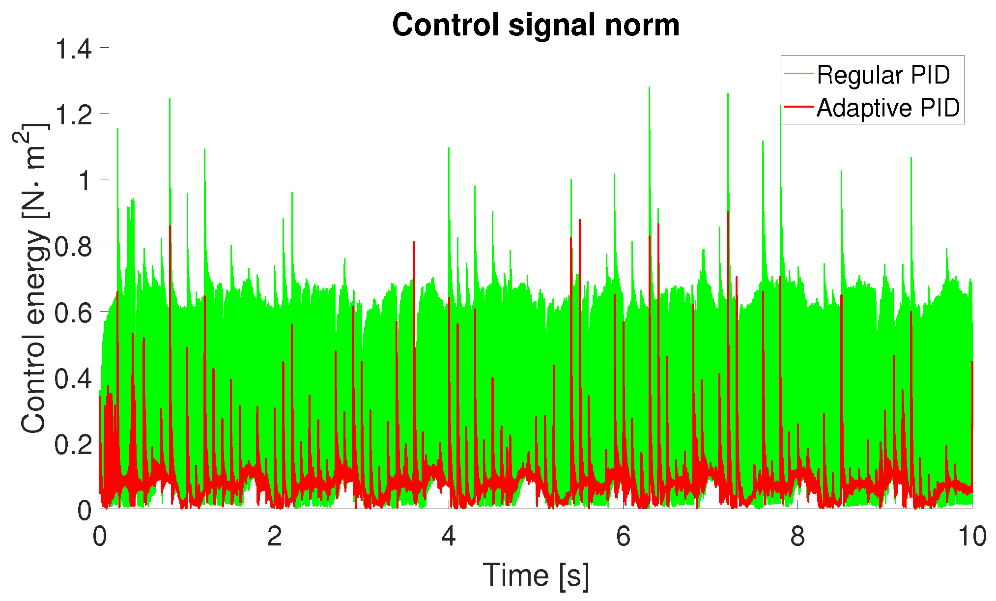
Figure 6).
Figure 6 also highlights the high energy consumed by the PID controller, while the adaptive controller is significantly smaller in comparison. The temporal evolution of the control norm motivates the inclusion of the adaptive controller for mobile robots, such as the biped structure considered in this study, with the linear actuators as driving elements.
Figure 7 and 
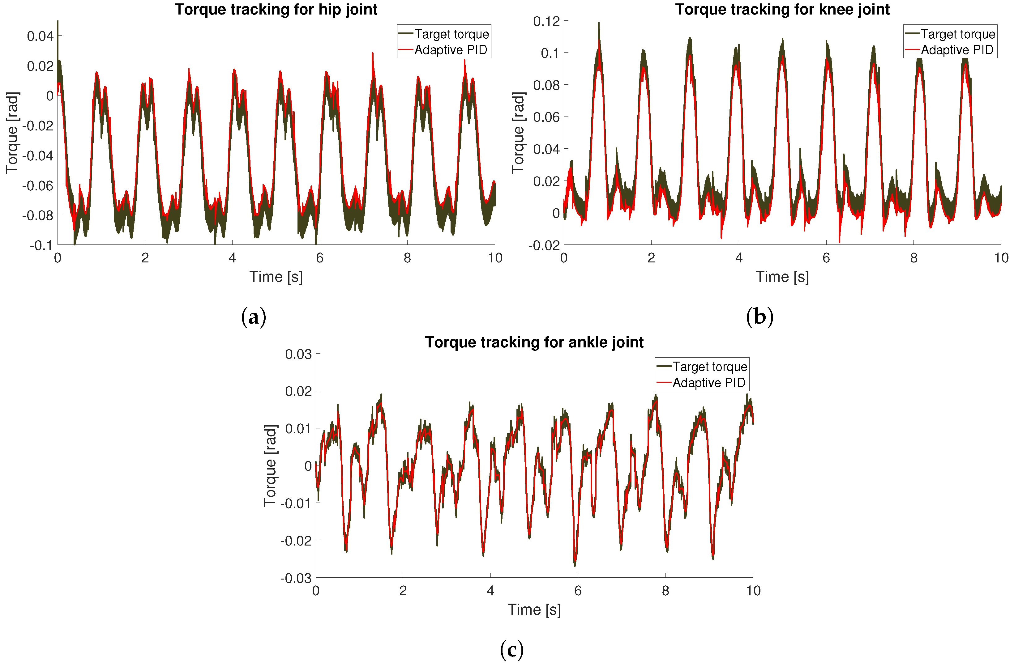
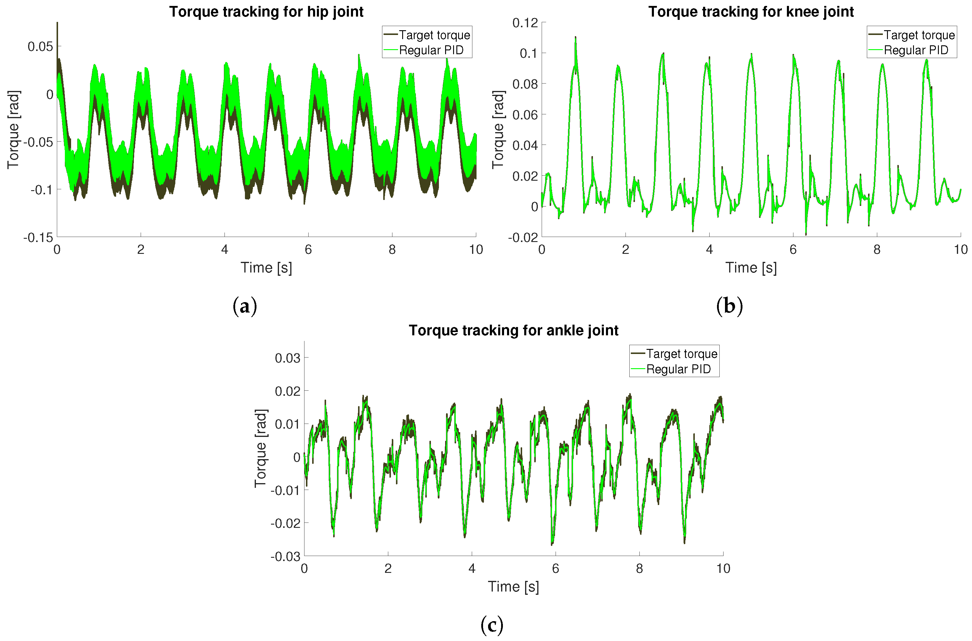
Figure 8 show the comparison of the torque enforced by both controllers, adaptive and PID forms. Notice that these reference torques are different due to the back-stepping formulation using either the PID or the adaptive control forms, which limits the ability to obtain a unified comparison of all three trajectories. The numerical outcomes correspond to the tracking of the reference PID and adaptive torques for hip, knee, and ankle articulations of the biped robot. In all these comparisons, the adaptive controller performs better in the tracking of the reference trajectories.
The reference tracking for the requested torques attains a similar time (0.12 s), which is smaller than the needed time for the position tracking. The equivalent quality tracking for torques in the PID case is not as good as in the case of the adaptive control form. Considering that the adaptive control structure forces a better tracking of the reference torque, the better tracking of the reference angular motion is even more justified. PID cannot provide an efficient tracking of the reference torques, highlighting the benefits of the suggested controller. This fact is confirmed for all three articulations in the biped robot structure corresponding to the calculated torques. The tracking errors for both torques produced by adaptive and PID converge to a particular invariant set that is part of this study’s main result for such variables. The individual comparisons of torques confirm that the adaptive controller tracks each reference torque with smaller oscillations around the reference torques. Notice also that tracking both torques at each articulation seems to correspond to the tracking of the reference position for each joint. This fact confirms the interplay between the linear actuator performance and the articulation motion in the biped robot joint.
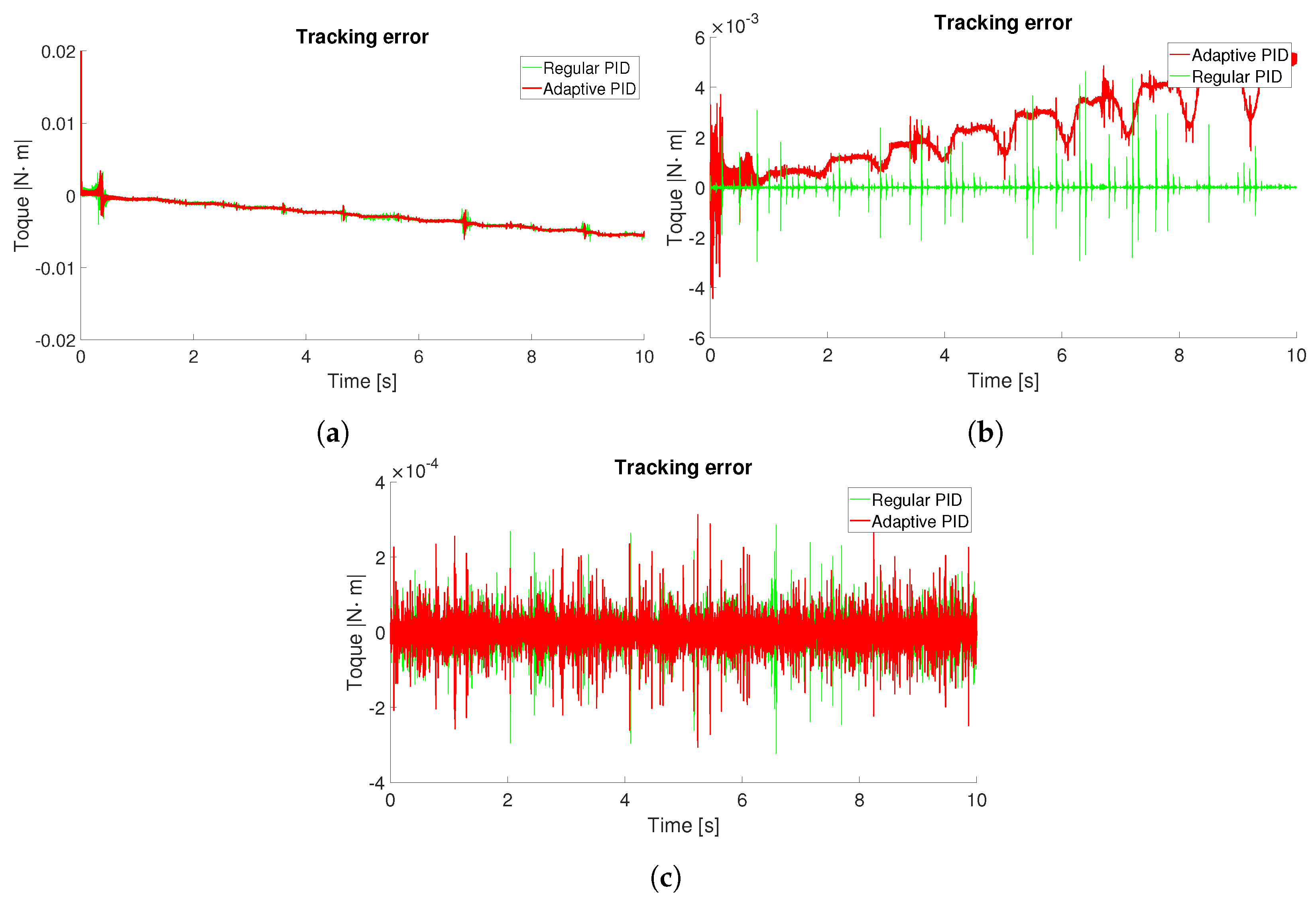
Figure 9 depicts the comparison of the torque’s deviation from their corresponding reference torques. This comparison shows a similar control tracking performance for both controllers (PID and adaptive forms) with similar quality. Nevertheless, the comparison seems to offer a similar quality to the torque tracking, but the improved position tracking exhibited by the adaptive form justifies its application for enforcing a more efficient gait cycle for biped robots.
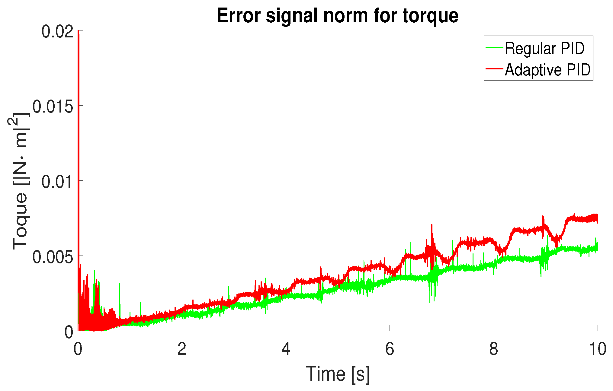
Figure 10 illustrates the temporal evolution of the Euclidean norm for the torque tracking error enforced with the pair of studied controllers (PID and adaptive structures). These norms are shown simultaneously in the same figure. Such comparison may highlight that the proposed controller drives the torque tracking error toward the origin by implementing both adaptive and PID forms. Nonetheless, both norms shown in this figure also prove that the adaptive form induces a good tracking of torque as the adaptive form does, but the adaptive formulation yields a better gait cycle developed by the suggested biped robotic device.
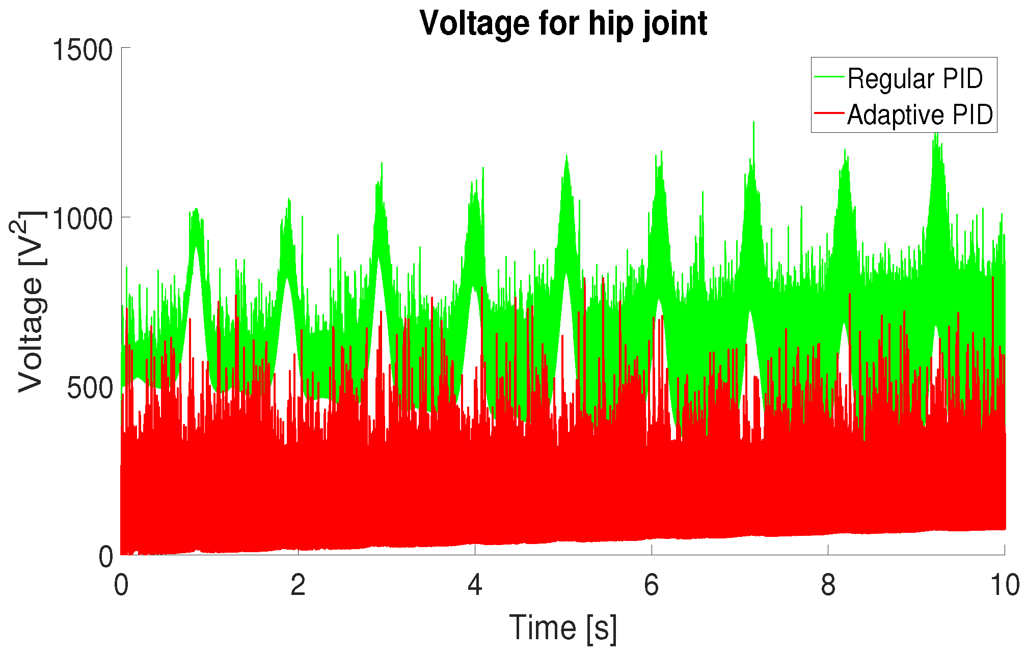
Figure 11 renders the square of voltage needed to drive the tracking of torque as well as the position. The temporal evolution of the voltage proves that the adaptive form requires half of the energy associated with the electrical source compared to the PID structure. This main characteristic is one of the most motivating aspects of the adaptive controller included in this study, considering the mobile nature of the biped robotic device.
With the aim of numerically evaluating the performance of both controllers, the L 2 norm of the control and error signals at each articulation (Table 1) were calculated.
The evaluation of the performance index J e was obtained as J e = 0 t f | δ 2 ( t ) | d t , where δ is the vector of errors at the hip, the knee and the ankle. In the same way, J c was obtained as J c = 0 t f | τ 2 ( t ) | d t , where τ is the vector of the control signals for the articulations. These comparisons also confirm the benefits of using the proposed controller with state-dependent gains.

6. Conclusions

The following are the final main remarks derived from this study:
  • This study proposes a new adaptive controller for a class of simplified biped robots with state restrictions that are handled with the application of state-dependent gains in a class of state feedback controllers.
  • The proposed controller was inspired by a traditional state feedback formulation that contains gains that are adjusted using the online evaluation of the tracking error and its derivative. Intending to simplify the implementation of the proposed controller, the application of a robust and exact differentiator based on the STA contributed to the state feedback, resulting in a class of output-based controllers with gains that also depend on the estimated derivative of the tracking error.
  • The stability analysis resulted in the time-dependent gain adjusting law, which may guarantee the tracking of the reference trajectories.
  • The application of the proposed controller justified the exertion of a regular gait cycle for a simulated biped robot that was developed in a virtualized version of the BRD that satisfies the dimensions of an averaged human being.
Proof. 
Consider the Lyapunov candidate function given by
V ξ , E , k ¯ 1 , k ¯ 2 = i = 1 n V i ξ i , E i , k ¯ 1 , i , k ¯ 2 , i V i ξ i , E i , k ¯ 1 , i , k ¯ 2 , i : = V 1 , i ξ i + V 2 , i E i + V 3 , i k ¯ 1 , i , k ¯ 2 , i
with V 1 , i ξ i = ξ i P 1 , i ξ i , V 2 , i E i = E i P 2 , i E i and V 3 , i k ¯ 1 , i , k ¯ 2 , i = π 1 , i k ¯ 1 , i 2 + π 2 , i k ¯ 2 , i 2 where k ¯ 1 , i = K P , i t K P , i * and k ¯ 2 , i = K D , i t K D , i * . The term referred to as ξ i is described by ξ i = | δ 1 , i | 1 / 2 sign δ 1 , i δ 2 , i . The time derivative of each function V i ξ i , e i , k ¯ 1 , i , k ¯ 2 , i is:
d d t V i t = 2 ξ i ( t ) P 1 , i d d t ξ i ( t ) + 2 E i P 2 , i d d t E i + 2 π 1 , i k ¯ 1 , i d d t k ¯ 1 , i + 2 π 2 , i k ¯ 2 , i d d t k ¯ 2 , i
Notice that V 1 , i ξ i is continuous; however, it is not differentiable if δ 1 , i = 0 . The ideas proposed by [20] are reconsidered here for handling the class of no regular Lyapunov functions. Let us continue the analysis of the second stage V 2 , i E i . From the calculus of the full-time derivative for the second function, one obtains d d t V 2 , i t = 2 E i t P 2 , i d d t E i t using Dini’s derivative. The direct substitution of d d t ξ i and d d t E i in the expression corresponding to the full-time derivative of V i t yields:
d d t V i t ξ i ( t ) P 1 , i A i , 1 + A i , 1 P 1 , i ξ i + E i t P 2 , i A 2 , i + α i I + A 2 , i + α i I P 2 , i E i t + E i t P 2 , i R 2 , i P 2 , i + Q 2 , i E i t α i V i t + γ i + 2 k ¯ 1 , i ( t ) π 1 , i d d t k ¯ 1 , i ( t ) + e i ( t ) M a P 2 , i E i ( t ) + 2 k ¯ 2 , i ( t ) π 2 , i d d t k ¯ 2 , i ( t ) + e i + n ( t ) M b P 2 , i E i ( t )
The differential inclusion (77) appears after the application of Young’s inequality X Y + Y X X Λ 1 X + Y Λ Y X, Y R s × q with 0 < Λ = Λ R s × s [21].
Considering the satisfaction of the condition for the existence of positive definite solutions for the given Lyapunov equations as well as the Riccati algebraic equations given in the theorem statement and in consideration of the adjusting laws for the gains k ¯ 1 , i ( t ) and k ¯ 2 , i ( t ) in (61), inclusion (77) transforms into: d d t V 2 , i t α i V 2 , i t + γ i .
Considering the solution of the inclusion for d d t V 2 , i t , and the application of the comparison Lemma, it led straightforwardly to V 2 , i t V 2 , i 0 e 2 α i t + γ i α i 1 e 2 α i t . Considering the case when the inclusion transforms to the equivalent ordinary differential equation, by redefining V i t as V i e q t , it can be proven that
V t i = 1 n V 1 , i 0 2 t i = 1 n κ 1 , i + i = 1 n V 2 , i 0 e α i t + γ i α i 1 e α i t
Clearly, when t T with T = i = 1 n V 1 , i 0 2 i = 1 n κ 1 , i , the following inequality can be justified
V t i = 1 n V 2 , i T e α i t T + i = 1 n γ i α i 1 e α i t T
If the upper limit is calculated, t results in lim ¯ t V t i = 1 n γ i α i . This result finishes the proof. □

Author Contributions

Conceptualization, K.R.-M.; Formal analysis, I.C. and W.-Y.L. All authors have read and agreed to the published version of the manuscript.

Funding

Ministry of Science and Higher Education of Russia within the Center “Supersonic” (agreement 075-15-2022-331 26 April 2022).

Institutional Review Board Statement

Not applicable.

Data Availability Statement

Not applicable.

Acknowledgments

The paper was prepared under the partial financial support of the Tecnologico de Monterrey, Institute of Advanced Materials for Sustainable Manufacturing.

Conflicts of Interest

The authors declare no conflict of interest.

References

  1. Ficht, G.; Behnke, S. Bipedal humanoid hardware design: A technology review. Curr. Robot. Rep. 2021, 2, 201–210. [Google Scholar] [CrossRef]
  2. Mikolajczyk, T.; Borboni, A.; Kong, X.W.; Malinowski, T.; Olaru, A. 3D printed biped walking robot. Appl. Mech. Mater. 2015, 772, 477–481. [Google Scholar] [CrossRef]
  3. Negrello, F.; Garabini, M.; Catalano, M.G.; Malzahn, J.; Caldwell, D.G.; Bicchi, A.; Tsagarakis, N.G. A modular compliant actuator for emerging high performance and fall-resilient humanoids. In Proceedings of the 2015 IEEE-RAS 15th International Conference on Humanoid Robots (Humanoids), Seoul, Korea, 3–5 November 2015; pp. 414–420. [Google Scholar]
  4. Kaneko, K.; Morisawa, M.; Kajita, S.; Nakaoka, S.; Sakaguchi, T.; Cisneros, R.; Kanehiro, F. Humanoid robot HRP-2Kai—Improvement of HRP-2 towards disaster response tasks. In Proceedings of the 2015 IEEE-RAS 15th International Conference on Humanoid Robots (Humanoids), Seoul, Korea, 3–5 November 2015; pp. 132–139. [Google Scholar]
  5. Mikolajczyk, T.; Mikołajewska, E.; Al-Shuka, H.F.; Malinowski, T.; Kłodowski, A.; Pimenov, D.Y.; Paczkowski, T.; Hu, F.; Giasin, K.; Mikołajewski, D.; et al. Recent Advances in Bipedal Walking Robots: Review of Gait, Drive, Sensors and Control Systems. Sensors 2022, 22, 4440. [Google Scholar] [CrossRef] [PubMed]
  6. Hashimoto, K. Mechanics of humanoid robot. Adv. Robot. 2020, 34, 1390–1397. [Google Scholar] [CrossRef]
  7. Lohmeier, S.; Buschmann, T.; Schwienbacher, M.; Ulbrich, H.; Pfeiffer, F. Leg Design for a Humanoid Walking Robot. In Proceedings of the 2006 6th IEEE-RAS International Conference on Humanoid Robots, Genova, Italy, 4–6 December 2006; pp. 536–541. [Google Scholar]
  8. Lim, H.O.; Takanishi, A. Biped walking robots created at Waseda University: WL and WABIAN family. Philos. Trans. R. Soc. Math. Phys. Eng. Sci. 2007, 365, 49–64. [Google Scholar] [CrossRef]
  9. Sugahara, Y.; Hashimoto, K.; Endo, N.; Sawato, T.; Kawase, M.; Ohta, A.; Tanaka, C.; Hayashi, A.; Lim, H.; Takanishi, A. Development of a Biped Locomotor with the Double Stage Linear Actuator. In Proceedings of the 2007 IEEE International Conference on Robotics and Automation, Rome, Italy, 10–14 April 2007; pp. 1850–1855. [Google Scholar]
  10. Gienger, M.; Loffler, K.; Pfeiffer, F. Towards the design of a biped jogging robot. In Proceedings of the 2001 ICRA. IEEE International Conference on Robotics and Automation (Cat. No.01CH37164), Seoul, Korea, 21–26 May 2001; Volume 4, pp. 4140–4145. [Google Scholar] [CrossRef]
  11. Haywood, M.; Sahin, F. A novel 3D printed leg design for a biped robot. In Proceedings of the 2017 12th System of Systems Engineering Conference (SoSE), Waikoloa, HI, USA, 18–21 June 2017; pp. 1–6. [Google Scholar]
  12. Qingxin, Z.; Hongmei, Z.; Fengxiang, W. The mathematical model of a novel linear actuator and its control strategy. In Proceedings of the 2007 Chinese Control Conference, Zhangjiajie, China, 26–31 July 2007; pp. 165–168. [Google Scholar]
  13. Lee, T.; Tan, K.; Huang, S.; Dou, H. Intelligent control of precision linear actuators. Eng. Appl. Artif. Intell. 2000, 13, 671–684. [Google Scholar] [CrossRef]
  14. Wang, J.; Huang, H.; Wang, Z.; Qin, F.; Zhao, H. Development and analysis of a dynamic model for parasitic motion principle piezoelectric actuator. Mech. Syst. Signal Process. 2021, 147, 107079. [Google Scholar] [CrossRef]
  15. Zahaf, A.; Bououden, S.; Chadli, M.; Chemachema, M. Robust fault tolerant optimal predictive control of hybrid actuators with time-varying delay for industrial robot arm. Asian J. Control 2022, 24, 1–15. [Google Scholar] [CrossRef]
  16. Gollapudi, A.M.; Velagapudi, V.; Korla, S. Modeling and simulation of a high-redundancy direct-driven linear electromechanical actuator for fault-tolerance under various fault conditions. Eng. Sci. Technol. Int. J. 2020, 23, 1171–1181. [Google Scholar] [CrossRef]
  17. Ames, A.D. Human-inspired control of bipedal walking robots. IEEE Trans. Autom. Control 2014, 59, 1115–1130. [Google Scholar] [CrossRef]
  18. Martínez-Fonseca, N.; Castañeda, L.Á.; Uranga, A.; Luviano-Juárez, A.; Chairez, I. Robust disturbance rejection control of a biped robotic system using high-order extended state observer. ISA Trans. 2016, 62, 276–286. [Google Scholar] [CrossRef] [PubMed]
  19. Levant, A. Higher-order sliding modes, differentiation and output-feedback control. Int. J. Control 2003, 76, 924–941. [Google Scholar] [CrossRef]
  20. Moreno, J.A.; Osorio, M. Strict Lyapunov functions for the super-twisting algorithm. IEEE Trans. Autom. Control 2012, 57, 1035–1040. [Google Scholar] [CrossRef]
  21. Poznyak, A.; Polyakov, A.; Azhmyakov, V. Attractive Ellipsoids in Robust Control; Springer: Berlin/Heidelberg, Germany, 2014. [Google Scholar]
Figure 1. Models considered for the BRD assuming the two configurations for the linear actuators forming a structure in the device. (a) Comparison of trajectory tracking performance between the proposed and PID controllers at the hip joint in the biped robot; (b) comparison of trajectory tracking performance between the proposed and PID controllers at the hip joint in the biped robot.
Applsci 12 08831 g001
Figure 2. Position tracking for each joint, comparing the proposed adaptive controller (red) scheme with a regular PID controller (green) for the hip (a), knee (b) and ankle (c).
Applsci 12 08831 g002
Figure 3. Tracking error signal comparison between the proposed adaptive controller (red) scheme and the regular PID controller (green) for the hip (a), knee (b) and ankle (c).
Applsci 12 08831 g003
Figure 4. Tracking error signals norm.
Applsci 12 08831 g004
Figure 5. Tracking control signal comparing the proposed adaptive controller (red) scheme with the regular PID controller (green) for the hip (a), knee (b) and ankle (c).
Applsci 12 08831 g005
Figure 6. Control signals norm.
Applsci 12 08831 g006
Figure 7. Comparison of the control evolution for the tracking problem based on the application of the adaptive controller (red) for the hip (a), knee (b) and ankle (c).
Applsci 12 08831 g007
Figure 8. Comparison of the control evolution for the tracking problem based on the application of the PID controller (green) for the hip (a), knee (b) and ankle (c).
Applsci 12 08831 g008
Figure 9. Torque evolution obtained with the application of a regular PID controller (green) and the proposed adaptive controller (red) for the hip (a), knee (b) and ankle (c).
Applsci 12 08831 g009
Figure 10. Norm of the tracking errors with the application of the regular PID and the adaptive controllers.
Applsci 12 08831 g010
Figure 11. Norm of the voltage evolutions with the application of the regular PID and the adaptive controller proposed in this study.
Applsci 12 08831 g011
Table 1. Norm L 2 of the error and control signals of both joints.
CharacteristicsController
AdaptivePID
J e , h 2.5892 × 10 4 9.0636 × 10 3
J c , h 7.4752 × 10 5 9.6471 × 10 6
J e , k 1.8016 × 10 4 1.1642 × 10 3
J c , k 8.1580 × 10 5 1.0912 × 10 6
J e , a 2.8016 × 10 4 1.2569 × 10 3
J c , a 9.0570 × 10 5 1.1258 × 10 6
Publisher’s Note: MDPI stays neutral with regard to jurisdictional claims in published maps and institutional affiliations.

