Research on Spatial and Temporal Evolution Trends and Driving Factors of Green Residences in China Based on Weighted Standard Deviational Ellipse and Panel Tobit Model

Abstract

The development of green residences is crucial to reducing energy consumption and carbon emissions of the construction industry. However, the study on the spatial distribution characteristics of green residences and its influencing factors has not attracted enough attention in the academic circles. Base on the panel database on the number of each star green residences and their driving factors at the municipal level from 2008 to 2016, this paper employed the Weighted Standard Deviational Ellipse model to reveal the spatial and temporal evolution features of green residences in China, creatively introduced an improved Gini coefficient (G′-score) to measure the green residences development in each city, and utilized the panel Tobit model and average marginal effect to identify the driving mechanisms and key factors of green residences from economy, society, the real estate market, policy and climate. The main conclusions show that: (1) China has formed a relatively stable and clear temporal and spatial evolution path since 2011, such as the center of gravity and coverage having moved to the west, and the direction of development trend having weakened; (2) China’s green residence is mainly distributed in the central and eastern regions, and the main direction layout is northeast–southwest; (3) the development of green residences is the result of the interaction of various factors, and the driving force of each factor varies greatly under the single action and the interaction; (4) the driving effects of the same factor on green residences with different star ratings are inconsistent in sign, magnitude, and significance, the same as for each factor under the same star rating.

1. Introduction

The construction industry plays an important role in improving people’s quality of life by creating architectural spaces and promoting national economic development. Meanwhile, the large volume of buildings contributes significantly to the country’s energy consumption, and Intergovernmental Panel on Climate Change (IPCC) reports that buildings expended 32% of the total global final energy use in 2010 [1]. The construction sector in China accounted for 46.5% of the energy consumed and 51.3% of the carbon emissions in 2018 [2]. Within this context, many countries have introduced the concept of green building and put it into practice to reduce the energy consumption and carbon emissions of the building industry [3].

As a high-quality building, green building can save energy, reduce carbon emission, protect the environment, and provide people with healthy, applicable, and efficient living and working spaces throughout the life cycle of a building [4,5,6,7]. When compared to traditional buildings, green buildings can reduce energy consumption by 30–60% [1], and decrease CO₂ emissions by 10% throughout their entire life cycle [8].

Green building is an important aspect of the urban sustainability movement in China and has been put into practice in multiple cities in the past decade [9]. However, the geographic distribution of the existing green buildings is uneven, and their certification grades have mainly low and medium star ratings [10]. For example, differences in economic and market factors among cities in China have resulted in spatial heterogeneity and star rating differences in the distribution of green buildings [11], and green building in China is diffusing from economically developed or high administrative level regions to low-level regions [12]. The development of green buildings is a complex issue in which local policies, economy, society, real estate, and climate conditions play critical roles and are interrelated. Additionally, green residence is an important branch of green building, and its certified area accounted for 61.19% of all green buildings at the end of September 2016. However, there are few studies on the temporal and spatial evolution of green residences and its driving factors in academia. To fill this gap, this paper provides an empirical analysis, and aimed to further research on the spatial patterns of the development of green residences with different star ratings in China, in order to fully reveal the spatial and temporal evolution law of green residence as far as possible, analyze its forming reasons in depth, and provide a solid empirical basis for the research of government green housing policy and the formulation of real estate enterprise development strategy in the future.

The remainder of this paper is organized as follows. Section 2 reviews the literature. Section 3 introduces the ranges, objects and methods used in this empirical study in detail. Section 4 studies the spatial and temporal evolution features of green residences in China by using the standard deviation ellipse model, and Section 5 mainly establishes a panel Tobit model to analyze the driving mechanism and key factors of green residences. Finally, Section 6 presents the conclusion.

2. Literature Review

In the current research results, there are few articles that take green residences as a separate concept to quantitatively study its spatial and temporal evolution characteristics and driving factors, especially from the perspective of different star levels. Since a green residence is a kind of green building with living function [13], the research results of scholars on the geographical distribution and driving factors of green buildings have reference significance for the study of green residences in this paper. Recently, there are differences in the geographical distribution of green buildings, and this difference is associated with local economic and social development levels, real estate market scale, policy environment, and climate conditions, which have become a growing consensus among scholars. Therefore, this paper mainly introduces the relevant research progress on the driving factors of green buildings.

In a number of cases, cities with active economies are more likely to adopt high-quality green buildings [14,15]. Kaza et al. [16] explored the spatial and temporal patterns of green buildings in the US and found strong evidence of the clustering of green buildings in areas with stronger economic performance. Furthermore, economically developed regions are able to attract highly educated and high-income residents with a strong environmental awareness [9], who are more prone to pay a premium for the high-quality and greener lifestyles brought by green buildings [17].

In terms of the social environment, there is a close link between local environmental awareness, demographic factors, residents’ income, housing and education level, and the development level of green buildings [18,19]. Lee et al. [20] carried out a multilevel analysis on the impact of political leadership on green buildings in 591 US cities and found that the local government’s support for environmental protection is strongly associated with the adoption of green buildings. Portney et al. [21] reported that there is a close relationship between family income, population, and the pursuit of sustainability in moderate-sized US cities. In addition, some academics [9,15,16,22] also confirmed that the demographic characteristics such as the income, housing, and educational conditions of individuals may also drive the promotion of green buildings.

The development level of the local real estate market, in terms of engineering technology, real estate price, and scale, is an important factor in driving green building development [9,16]. Areas with extraordinary technical levels in terms of construction and lower green building premiums can reduce the barriers to the spread of green buildings [23,24]. When compared to traditional housing, the sales premium of green residences is one of the factors most concerned by buyers, and a city with a high level of construction technology can effectively reduce the premium of green residences in its region [25]. It should be noted that there is a remarkable correlation between the number of Leadership in Energy and Environmental Design (LEED)-certified projects and the size of the real estate market in the United States [14,22], but the performance of the scale of the real estate market on the green residence development may not be significant in China [26].

A city’s capacity to implement policies, in terms of both public incentives and mandates, is an important factor in driving green building initiatives [18]. Delmas et al. [27] empirically concluded that mandatory external policies would urge companies to implement green management strategies. Karkanias et al. [28] studied the green building market in Greece and found that insufficient policy incentives had hindered the promotion of green building. Franco et al. [29] recommended that compulsory and incentive policies should be together in the development of the green building sector in Metro Manila.

In addition, the climate condition as one of the primary considerations in architectural design and construction also plays a role in the adoption of green buildings [30].

Finally, there are some differences in the distribution and driving factors of the different stars of green buildings, and studies on green residences are particularly prominent [31].

3. Research Ranges, Objects and Methods

In this paper, the number of green residences with different stars in various cities in China from 2008 to 2016 was collected and sorted, and the spatial and temporal evolution trend of green residences in China was explored by using the weighted standard deviation ellipse model. The development levels of green residences were estimated by an improved Gini coefficient of green building development (G′-score), and the panel Tobit model and average marginal effect were used to quantitatively analyze the influence of 21 driving factors on the G′-score in 42 cities with a greater number of green residences.

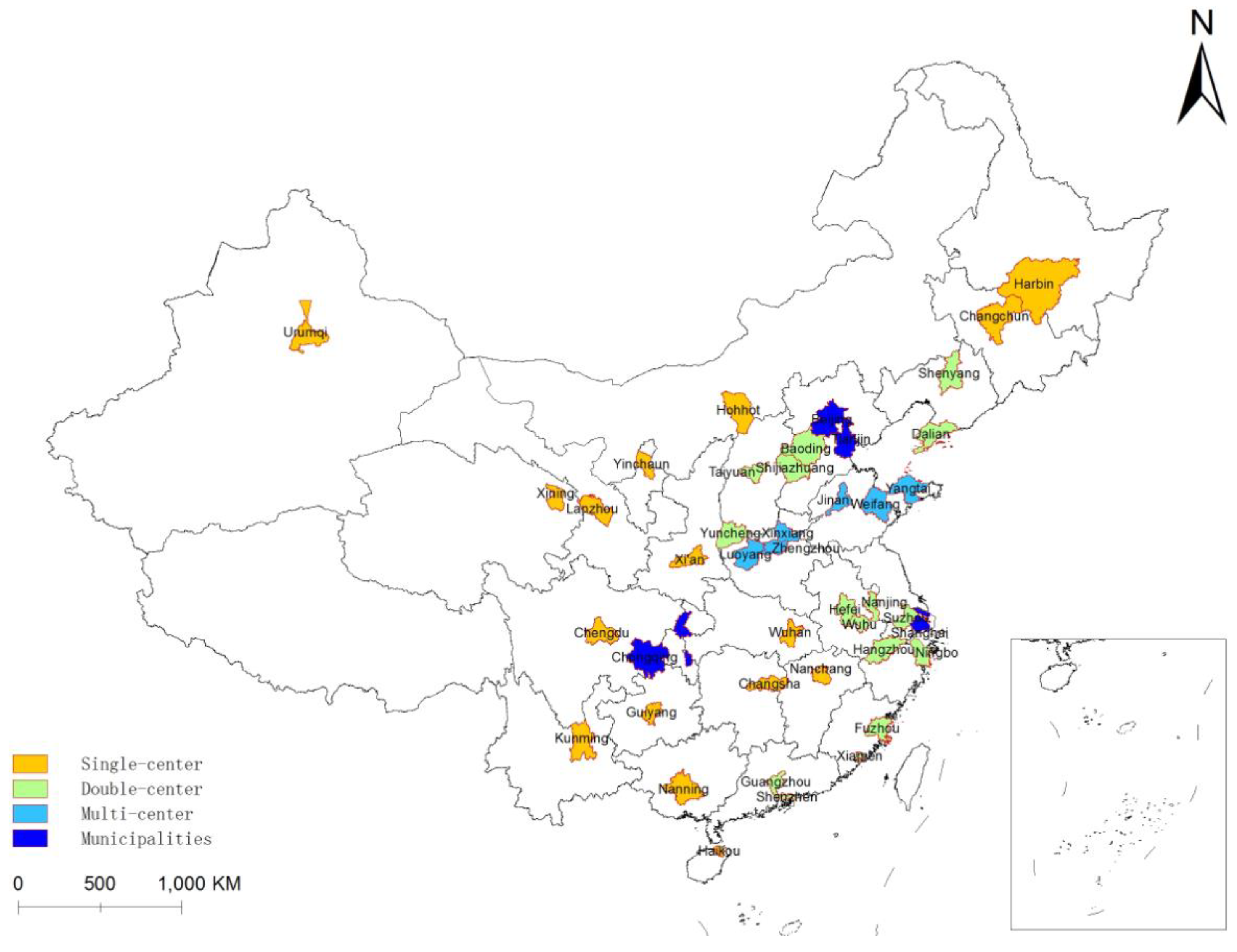
3.1. Research Ranges

The Green Building Evaluation Standard (GBES) was issued by the Ministry of Housing and Urban–Rural Development of China in 2006. Before that, green buildings were limited to academic studies and rarely put into practice [9]. With the improvement in the implementation rules, the number of GBES certification projects in China began to grow rapidly in 2008 [12,32]. From 2008 to 2016 (at the end of September), a total of 2124 residences which were distributed in 207 cities in China (excluding Hong Kong, Macao, and Taiwan) met the GBES and obtained a green building label, and each certified green residence is listed on the website ‘Chinese Green Building Evaluation Label’ (CGBEL) (http://www.cngb.org.cn/, Accessed on 20 July 2021). This paper explored the spatial and temporal evolution characteristics of the 2124 green residences based on their distribution in various cities.

In previous studies [33], the authors of this paper used the development concentration index to compare the number of green residences in cities in various provinces of China (except Tibet), and found that green residences were mostly concentrated in provincial capitals or economically and socially developed cities, and defined the leading cities as those cities which have a number of green residences totalling more than 50% of the total in the province, or far more than any other cities in the province. In total, 42 leading cities with a greater number of green residences were defined, as shown in Figure 1.

Table 1. Number of green residences over the years (2008–2016).

Star Level	2008	2009	2010	2011	2012	2013	2014	2015	2016
42 Leading Cities
Total	3	7	46	158	281	513	817	1210	1335
One-star	2	3	13	50	93	179	310	501	565
Two-star		2	23	61	123	245	361	528	572
Three-star	1	2	10	47	65	89	146	181	198
China
Total	4	8	53	191	379	752	1252	1845	2035
One-star	3	4	14	61	127	260	471	757	850
Two-star		2	27	76	169	376	591	847	919
Three-star	1	2	12	54	83	116	190	241	266
Ratio
Total	75%	88%	87%	83%	74%	68%	65%	66%	66%
One-star	67%	75%	93%	82%	73%	69%	66%	66%	66%
Two-star		100%	85%	80%	73%	65%	61%	62%	62%
Three-star	100%	100%	83%	87%	78%	77%	77%	75%	74%

Data source: http://www.cngb.org.cn/.

shows the number and proportion of different star green residences in China and 42 leading cities over the years. The proportion of the green residence counts owned by the 42 cities of has been decreasing year by year, indicating that the growth of green residences in China is diffuse and nonuniform. At the same time, for the leading cities with better green residence development in each province, the number of green residences owned by them has always been higher than 60% of the total number, especially for the proportion of three-star green residences, which has reached more than 70%. Therefore, this paper selected the 42 leading cities to study the driving factors of green residence development.

3.2. Research Objects

This paper selected the improved Gini coefficient to measure the development level of green residences, and chose 21 influence factors from the perspectives of society, economy, the real estate market, government and natural climate to study the driving mechanisms and key driving factors of green housing in China.

3.2.1. Green Residence Development Indicator

Identifying the most appropriate criterion for green residences development is not straightforward. Some quantitative studies on the driving factors of green residences selected the number or area of green residences as a standard to measure the level of development [10,34], but this cannot reflect the impact of the scale of local real estate development on green residences. Based on a study by Qiu et al. [12], this paper put forward an improved Gini coefficient of green building development (labeled G′-score) to represent the annual measure of green residence development in each city, and the G′-score is defined as follows:

$${G^{\prime }}_{it}\equiv Q_{it}/X_{it}$$

(1)

Here, $Q_{it}=q_{it}/Q_t$ represents the ratio of the amount of green residences owned by city i to the total amount in the 42 leading cities in year t; $X_{it}=s_{it}/S_t$ is the proportion of the newly commenced area of commercial residential buildings in city i to the total newly commenced area of commercial residential buildings in the 42 leading cities from 2008 to year t. Due to the fact that approximately 96% of the 1210 green residences samples selected in this article obtained the design labels, this article selected the newly commenced area of commercial residential housing to represent the scale of the local housing market.

Using the G′-score, if $G^{\prime }=$ 0, this indicates that the city does not have green residences in this year. If $G^{\prime }=$ 1, this shows that the city has the same proportion of green residences and new housing space among the 42 leading cities in that year, and the development of green residences is appropriate and balanced in that city. If $G^{\prime }>$ 1, this illustrates that the development of green residences in this city is above the average level of the 42 cities, and the higher the value, the better the green residence development. If $G^{\prime }<$ 1, this illustrates that the development of green residences in this city is below the average level of the 42 cities, and the lower the value, the worse the green residences development. To show how the G′-score is different from a simple proportion of the green residence number to the total, this paper took Beijing and Weifang’s green residences of a two-star level in 2015 as an example. Due to the fact that both the numbers of green residences in these two cities were 27 and the proportion of total green residences was 5.11%, this study assumed that their development was consistent. However, Beijing and Weifang had built 130 and 84 million square meters of commercial housing from 2008 to 2015, respectively. Clearly, there was a large difference in the scale of the real estate market between the two cities, and the proportion of green residences in Weifang’s new residential buildings was larger. In this paper, they obtained different G′-scores, which quantitatively represent the gap in their development levels of green residences.

3.2.2. Driving Factors for Green Residences Development

Overall, the existing literature suggested that the adoption of green residence is likely to be associated with a number of factors. Based on the literature summary, this document constructed 21 driving factors for green residence development from five aspects: economic factors, social environment, the real estate market, government measures, and the climatic condition (see

Table A1. Driving factors of green residences in China.

Dimension	Code	Driving Factors
Economic Factor	GDP	Gross domestic product
	RGPB	Revenue in the general public budgets
Social Environment	EECEP	Expenditure on energy conservation and environmental protection
	AQI	Air quality index
	PRP	Permanent resident population
	UR	Urbanization rate
	UCDI	Urban per capita disposable income
	UCHA	Urban Per capita housing area
	PPEU	Proportion of population with an education above university level
The Real Estate Market	COV	Cross-output value of the construction industry
	ICR	Investment in commercial residences
	CRCNA	Commercial residential construction area
	CRCMA	Commercial residential completion area
	CRSA	Commercial residential sale area
	CRP	Commercial residential price
Government Measure	CP	Compulsory policy
	EIP	Economic incentive policy
	NEIP	Non-economic incentive policy
	DE	Demonstration effect
	GE	Guidance effect
Climatic Condition	CRA	Climate regionalization for architecture

for more details in Appendix A).

Unless otherwise specified, the economic, social and real-estate-related data in this paper were mainly collected from the statistical yearbooks, communiques and other official sources of various cities from 2009 to 2017, and a few missing data were supplemented by interpolation. First, GDP and RGPB were used to measure the city’s economic development level and financial condition. Second, this study measured the local levels of social development from environmental awareness, demographic factor, living standards, and the education level of people. For instance, EECEP measures the local government’s environmental awareness, PRP and UR represent demographic factors, UCDI and UCHA denote people’s living standards, and PPEU, which is supplemented by interpolation based on data from the sixth and seventh census bulletins of each city, represents the educational level of the inhabitants. Third, local real estate market conditions include the technical level of construction, the size of the market, and the sales price of commercial housing [11]. This paper selected COV to measure the technical level of the local construction industry, and used ICR, CRCNA, CRCMA and CRSA to represent the scale of the local real estate market and collected CRP from the China Real Estate Index system (https://www.cih-index.com/research/indexstudy, Accessed on 18 May 2021).

Government measures, including coercive measures, incentive policy, guidance, and demonstrations, appear to be a significant factor for the adoption of green residences by development enterprises. This study searched CGBEL and local government websites and screened local regulations, government regulations, normative documents, and technical standards that contained green building-related policies. This paper classified the content of these policies from the aspects of coercive measures, incentive policies, and guidance effects to construct qualitative variables of government measures. Economic incentive policies refer to the government giving certain incentives to enterprises to obtain additional economic income, which mainly refer to financial subsidies, the reduction or exemption of urban ancillary fees, tax incentives, plot ratio, land planning, sales, etc. Non-economic incentive policies are the government’s support for enterprises adopting green residences in project approval, awarding, enterprise qualification, and credit. The mandatory policy is mainly that the government requires that new commercial residential buildings that meet certain conditions must be enforced with no less than a one-star rating. The guiding role is that the government has issued standard documents, such as local evaluation standards, implementation rules, and technical guidelines, according to local conditions. This paper counted the affordable housing projects of newly built public rental housing and affordable housing funded by local financial investments, published by CGBEL, and we defined them as demonstration effects. If a city has these measures, the variable was one, or else it was zero.

According to the Chinese Code for Design of Civil Buildings (GB50352-2019), the 42 leading cities experience severe cold, cold, hot summers and cold winters, hot summers and warm winters, and mild areas, and this article assigned their variable values from one to five. The descriptive statistics of the values of the 21 driving factors are shown in

Table 2. Descriptive statistics on the driving factors and variables of green residences in China.

Dimension	Factor	Unit	Obs.	Mean	Min.	Max.
Economic Factor	GDP	CNY 100 million	336	5314.3	439.94	25,643.47
	RGPB	CNY 100 million	336	616.18	29.46	5519.5
Social Environment	EECEP	CNY 100 million	336	32.98	0.5	708.83
	AQI	%	336	81%	12%	100%
	PRP	10,000 persons	336	827.89	165.43	3016.55
	UR	%	336	66%	26%	100%
	UCDI	CNY	336	25,827.19	11,290.5	52,962
	UCHA	sq. m	336	30.27	12.81	47.6
	PPEU	%	336	18%	5%	37%
The Real Estate Market	COV	CNY 100 million	336	1544.26	73.11	8436.7
	ICR	CNY 100 million	336	556.09	22.7	2451.37
	CRCNA	10,000 sq. m	336	3986.63	461.1	20,294.49
	CRCMA	10,000 sq. m	336	683.12	28.13	3386.35
	CRSA	10,000 sq. m	336	903.42	100.78	4477.71
	CRBP	CNY/sq. m	336	9254.6	1466.06	35,822.92
Government Measure	CP		336		0	1
	EIP		336		0	1
	NEIP		336		0	1
	DE		336		0	1
	GE		336		0	1
Climatic Condition	CRA		42		1	5

Obs. = number of observed variables; Min. = minimum value; Max. = maximum value; sq. m = square meter.

.

3.3. Research Methods

This study used the weighted standard deviation ellipse method to evaluate the spatial and temporal trends of green residences in China. In the driving factors analysis, this paper first adopted the Spearman’s correlation coefficient to verify the close connection between the selected driving factors and the G′-score, and then employed the panel Tobit model and average marginal effect value to identify the driving mechanism and key factors of green residences development in China.

3.3.1. Weighted Standard Deviation Ellipse

The standard deviational ellipse method (SDE) is a statistical method that can accurately reveal the spatial distribution characteristics of research elements, and is widely used to explore and analyze the spatial variation trends of geographic elements such as the gravity center, distribution, orientation and shape [35]. Generally, the SDE model contains ellipse center coordinates, rotation angle, major and minor axe standard deviations for four basic parameters, and displays the parameter calculation results in ellipses, which more intuitively describes the spatial and temporal evolution trends of geographic elements from multiple angles [36]. In this work, the overall contour and evolution direction of the spatial distribution of green residences are reflected by the moving trajectory of the center of gravity, the distribution direction and the diffusion range of the ellipse [37].

This paper employed the weighted ellipse center coordinates and took the number of green residences owned by each city as the weight. The moving trajectory of the center of gravity was observed to understand the direction of green residences in China. The formula used to calculate the weighted ellipse center coordinates is as follows:

$$\left(\overline{x},\overline{y}\right)=\left[\left({\displaystyle \sum _{i=1}^n{w}_i{x}_i}/{\displaystyle \sum _{i=1}^n{w}_i}\right),\left({\displaystyle \sum _{i=1}^n{w}_i{y}_i}/{\displaystyle \sum _{i=1}^n{w}_i}\right)\right]$$

(2)

where, $\left(x_i,y_i\right)$ represents the spatial coordinates of city i, $w_i$ denotes the weight of green residences’ number of city i.

The rotation angle represents the angle at which the major axis rotates clockwise from due north and reflects the main trend direction of green residences’ distribution. The calculation formula is as follows:

$$\tan \theta =\frac{\left({\displaystyle \sum _{i=1}^n{w}_i^2{\tilde{x}}_i^2-{\displaystyle \sum _{i=1}^n{w}_i^2{\tilde{y}}_i^2}}\right)+\sqrt{{\left({\displaystyle \sum _{i=1}^n{w}_i^2{\tilde{x}}_i^2-{\displaystyle \sum _{i=1}^n{w}_i^2{\tilde{y}}_i^2}}\right)}^2+4{\displaystyle \sum _{i=1}^n{w}_i^2{\tilde{x}}_i^2{\tilde{y}}_i^2}}}{2{\displaystyle \sum _{i=1}^n{w}_i^2{\tilde{x}}_i{\tilde{y}}_i}}$$

(3)

where, ${\tilde{x}}_i$ and ${\tilde{y}}_i$ denote the coordinate deviations from the spatial coordinates of city i to the weighted ellipse center, respectively. The other symbols are the same as Equation (2).

Then, the standard deviations along the x axis and y axis are defined as the major and minor axes of the spatial distribution, respectively, as shown in Equations (4) and (5). The major axis reflects the main trend direction of green residence spatial distribution, and the changes in the dimensions of the major and minor axes indicate a contraction or expansion of the green residence spatial distribution direction. The formulas are as follows:

$${\sigma }_x=\sqrt{\frac{{\displaystyle \sum _{i=1}^n{\left(w_i{\tilde{x}}_i\cos \theta -w_i{\tilde{y}}_i\sin \theta \right)}^2}}{{\displaystyle \sum _{i=1}^n{w}_i^2}}}$$

(4)

$${\sigma }_y=\sqrt{\frac{{\displaystyle \sum _{i=1}^n{\left(w_i{\tilde{x}}_i\sin \theta -w_i{\tilde{y}}_i\cos \theta \right)}^2}}{{\displaystyle \sum _{i=1}^n{w}_i^2}}}$$

(5)

where the symbols are the same as Equation (3).

According to the basic parameters of the ellipse, two additional parameters, namely, the ellipse area and axial ratio (the ratio of minor and major axes), were calculated in this paper to reflect the range and shape of the spatial distribution of green residences. The smaller the axial ratio, the more obvious the directionality of the spatial distribution of green residences. If the axial ratio is equal to 1, it means that there is no directional feature.

3.3.2. Spearman’s Correlation Analysis

Spearman’s correlation, as a nonparametric correlation estimator, is widely used in the applied sciences [38]. To ensure that the driving factors selected in this paper can promote the green residences development, this study used the Spearman’s correlation coefficient to evaluate the degree of correlation between the driving factors and the G′-scores of the green residences with different star ratings [39], as most of the driving factors do not conform to the normal distribution [40]. The Spearman’s coefficient is typically designated as $\rho$; if $\rho >0$, this indicates a positive correlation between two variables, otherwise it is a negative correlation. Note that the size of the correlation coefficient must be tested to verify whether it is manifest or not, which cannot be used directly to determine whether it reaches a significance level [41]. The coefficient is defined as follows:

$$\rho =\frac{{{\displaystyle \sum }}_i\left(x_i-\overline{x}\right)\left(y_i-\overline{y}\right)}{\sqrt{{\left(x_i-\overline{x}\right)}^2{\left(y_i-\overline{y}\right)}^2}}$$

(6)

where, $x_i$ is the G′-score of green residence in city i; $y_i$ is the value of this driving factor in city i; $\overline{x}$ and $\overline{y}$ are the means of $x_i$ and $y_i$, respectively.

3.3.3. Panel Tobit Regression Analysis

To identify the driving factors for the adoption of green residences, this paper proposed the hypothesis that these factors are linearly related to the green residence development in cities and their driving forces are related to the star levels of green residences. This study constructed a short panel empirical model of the effects of the aforementioned economic factors, social environment, the real estate market, government measures, and climatic condition on the development of green residences with different star ratings in 42 cities.

As an innovation, green residence is currently in the early stage of development [9], and 55% of the 1008 quantity samples of green residences selected in this paper had a value of 0. In this case, the OLS model cannot obtain a consistent estimation, whether using the entire sample or excluding the subsample after zero [42]. To address this problem, this paper treated the G′-score of green residences as censored data and adopted the panel Tobit model to construct the regression equation. If city i did not have a green residence in year t, this study specified it as the left censored value, and the baseline structure for a left censored Tobit model with panel data can be described as follows:

$$\begin{array}{c}{y}_{it}^{*}={\alpha }_i+{x^{\prime }}_{it}\beta +d_{it}\gamma +w_j+{\epsilon }_{it}\\ y_{it}=\{\begin{array}{ll}{y}_{it}^{*}& if y_{it}^{*}>0\\ 0& if y_{it}^{*}\le 0\end{array}\end{array}$$

(7)

where $y_{it}$ represents the G′-score of green residences in city i in year t; ${\alpha }_i$ is the intercept term, reflecting the heterogeneity of the individual differences in cities; $x_{it}$ is a independent variable including economic, social, and real estate market. To alleviate the influence of heteroscedasticity, autocorrelation, and multicollinearity of explanatory variables, this paper adopted logarithmic processing for absolute value variables. $d_{it}$ is a dummy variable representing government measures; $\beta$ and $\gamma$ are vectors of estimated coefficients; $w_j$ is the climate region’s fixed effect; ${\epsilon }_{it}$ is the robust standard error term, ${\epsilon }_{it}~N\left(0,{\sigma }_{\epsilon }^2\right)$.

3.3.4. Average Marginal Effect

The estimation parameters of the Tobit model cannot reflect the actual change in the dependent variable when the independent variables have a unit increase. To evaluate the effect of how independent variables affect the green residential development, this paper calculated the average marginal effects of a unit change in the ith independent variable in year t on the probability that an observation is above zero, as carried out in [43]. The formula is as follows:

$$\frac{\partial E\left(y|y>0\right)}{\partial x_{it}}=1-\frac{Z\phi \left(Z\right)}{\Phi \left(Z\right)}-\frac{\phi {\left(Z\right)}^2}{\Phi {\left(Z\right)}^2}$$

(8)

where

$$Z=\frac{X\beta }{{\sigma }_{\epsilon }}=\frac{X\beta }{\sqrt{{\sigma }_{\nu }^2+{\sigma }_{\mu }^2}}$$

(9)

and $\Phi \left(Z\right)$ is the cumulative normal distribution function; $\phi \left(Z\right)$ is the standard normal density function; $X$ is the vector of independent variables, β is a vector of estimated coefficients, ${\sigma }_{\mu }$ is the standard deviation of the random effect; ${\sigma }_{\upsilon }$ is the standard deviation of the disturbance term. The average marginal effect is the arithmetic average of the marginal effect for each sample observation.

4. The Spatial and Temporal Evolution Trends of Green Residences in China

Using ArcGIS 10.8 software, this paper calculated the SDE model of green residences at the municipal level in China from 2008 to 2016 according to Equations (2)–(5), and obtained the parameters table of the standard deviational ellipse (

Table 3. The standard deviation ellipse parameters of green residences in China.

Grade	Year	Weighted Ellipse Center Coordinate	Rotation Angle (°)	Major Axis Standard Deviation (km)	Minor Axis Standard Deviation (km)	Ellipse Area (10,000 sq.km)	Axial Ratio
One-star	2008	132.06° E, 35.63° N	93.05	783.15	211.26	12.99	0.27
	2009	132.85° E, 35.82° N	89.96	745.7	200.32	11.73	0.27
	2010	130.43° E, 36.83° N	50.77	1670.89	1032.27	135.47	0.62
	2011	130.06° E, 36.49° N	30.8	1777.37	1067.9	149.07	0.6
	2012	129.80° E, 36.46° N	23.9	1826.19	1010.28	144.9	0.55
	2013	129.30° E, 35.66° N	21.38	1848.52	1023.18	148.55	0.55
	2014	128.97° E, 36.43° N	20.83	1875.09	1095.09	161.27	0.58
	2015	128.56° E, 36.78° N	24.3	1822.82	1172.6	167.87	0.64
	2016	128.32° E, 36.93° N	24.78	1766.21	1191.37	165.26	0.68
Two-star	2009	130.11° E, 48.01° N
	2010	129.69° E, 39.94° N	122.86	1970.71	1286.33	199.1	0.65
	2011	130.00° E, 38.79° N	15.58	1834.83	1437.41	207.14	0.78
	2012	130.55° E, 39.53° N	11.34	1701.76	1127.75	150.73	0.66
	2013	129.36° E, 40.19° N	178.7	1496.48	1267.53	148.98	0.85
	2014	129.17° E, 40.01° N	9.67	1460.54	1193.42	136.9	0.82
	2015	129.09° E, 40.22° N	29.34	1598.1	1391.81	174.69	0.87
	2016	129.16° E, 40.16° N	29.28	1575.33	1366.12	169.02	0.87
Three-star	2009	130.68° E, 31.17° N
	2010	129.43° E, 38.08° N	125	2517.72	1406.03	278.03	0.56
	2011	129.97° E, 38.03° N	172.58	1677.45	1418.83	186.93	0.85
	2012	130.72° E, 39.28° N	13.62	1832.96	1254.53	180.6	0.68
	2013	129.68° E, 39.25° N	14.59	1814	1470.78	209.54	0.81
	2014	129.43° E, 19.16° N	3.92	1748.49	1689.81	232.06	0.96
	2015	128.92° E, 39.03° N	119.38	1866.51	1760.94	258.15	0.94
	2016	129.07° E, 38.97° N	125.2	1806.08	1753.6	248.75	0.97

) and the visualization results of the standard deviational ellipse at different star levels (Figure 2, Figure 3 and Figure 4), and revealed the spatial evolution trends of the spatial distribution direction, range and shape of green residences in China.

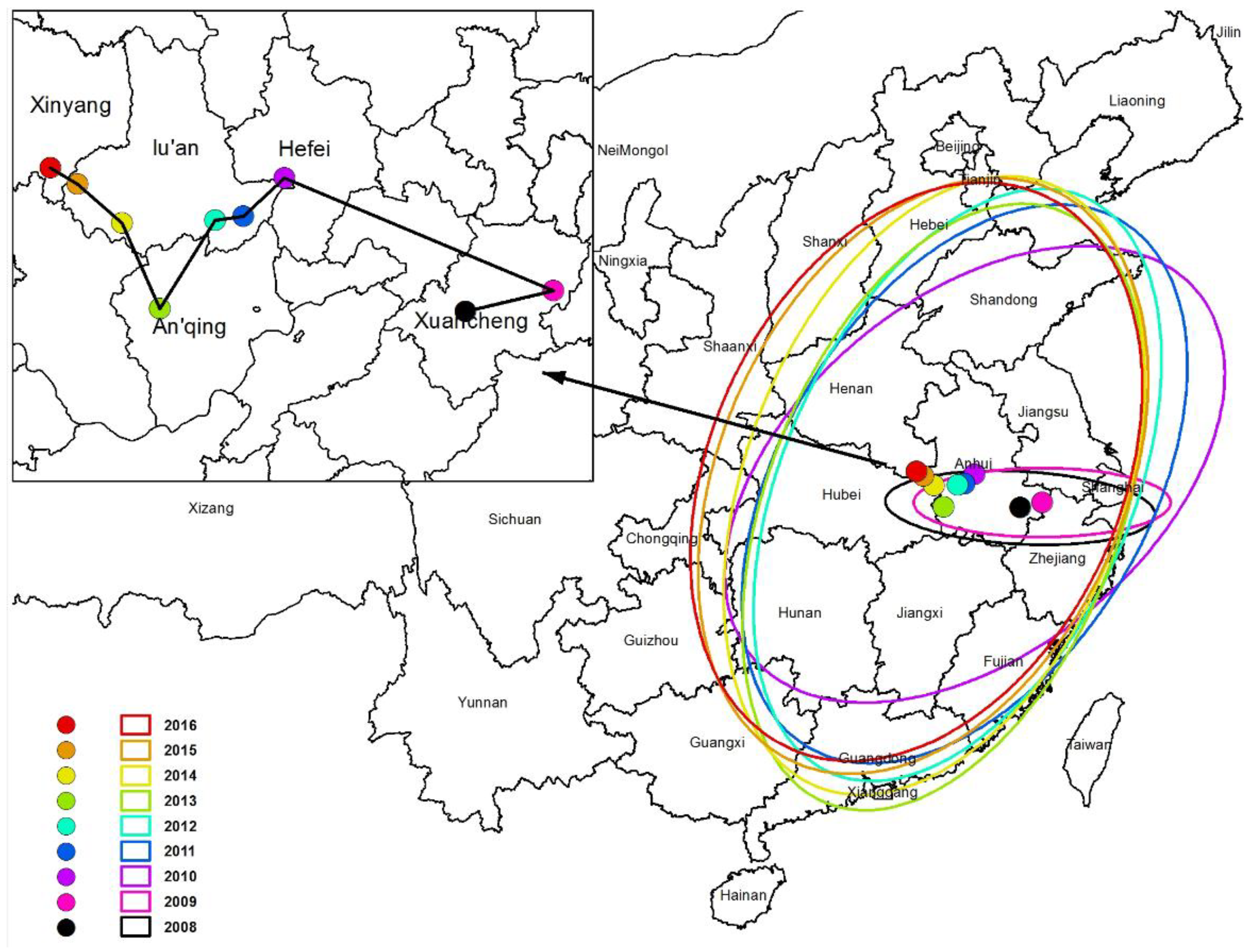
4.1. The Spatial and Temporal Evolution of One-Star Green Residences

According to the visualization results shown in Figure 2, the spatial and temporal evolution of one-star green residences can be divided into two stages.

During 2008 to 2009, the center of gravity was always in Xuancheng in Anhui province, and only shifted 81.80 km to the northeast. The weighted standard deviation ellipses only cover an area of less than 0.13 million km² in the Yangtze River Delta, showing an obvious east–west distribution pattern. The major and minor axes standard deviations were shortened by 37.45 km from 783.15 to 745.70 km and 10.94 km from 211.26 to 200.32 km, respectively, and the axial ratio remained unchanged at 0.27, indicating that the direction and shape of the spatial distribution change trend of one-star green residences were not significant. This is because before 2010, except for Wuhan, Ningbo, Wuxi and Shanghai, there were no one-star green residences in other cities.

During 2010 to 2016, the center of gravity moved gradually from east to west with slight fluctuations in the north–south direction with a displacement of 358.5 km. It can be found that during this period, the development speed of one-star green residences in the northern and southern regions of China was similar, but the development rate in the western region was faster than in the eastern region, which made the centers of gravity move westward every year. There was a obvious trend of southward movement in 2013, which was due to the rapidly development of one-star green residences in Guangdong province. The area of ellipse fluctuates between 135.47 and 167.87 km², covering mainly the eastern coastal regions of Shandong, Jiangsu, Shanghai, Zhejiang, Fujian and Guangdong, and the central regions of Hebei, Henan, Hubei, Hunan, Anhui and Jiangxi. It indicated that cities in these regions had a relatively large number of one-star green residences. It’s worth noting that the ellipse began to spread significantly westward, covering parts of Shanxi, Shaanxi, Chongqing, Guizhou and Guangxi from 2013. This is mainly related to the vigorous development of one-star green residences in central and western regions in China. The rotation angle decreased by 29.94° from 50.77° in 2014 to 20.83° in 2014, and then increased to 24.78° in 2016. It is obvious that the ellipse has a northeast–southwest distribution pattern. The major axis standard deviation increased first and then decreased. It first increased from 1670.89 km in 2010 to 1875.09 km in 2014, and then decreased to 1766.21 km in 2016, with a fluctuation of 204.2 km. The minor axis standard deviation had a more obvious fluctuation. The minimum value appeared in 2012 with 1023.18 km, and the maximum value appeared in 2016 with 1191.37 km, with a difference of 181.09 km, and the axial ratio also fluctuated around 0.6. It can be seen that the one-star green residences were mainly distributed in the central and eastern regions in China during the study period, and this presents the main trend of development in the northeast–southwest direction. However, due to the rapid development of one-star green residences in the western region, the east–west expansion speed of the ellipse range was obviously greater than that in the north–south direction, and the center of gravity moved westward obviously.

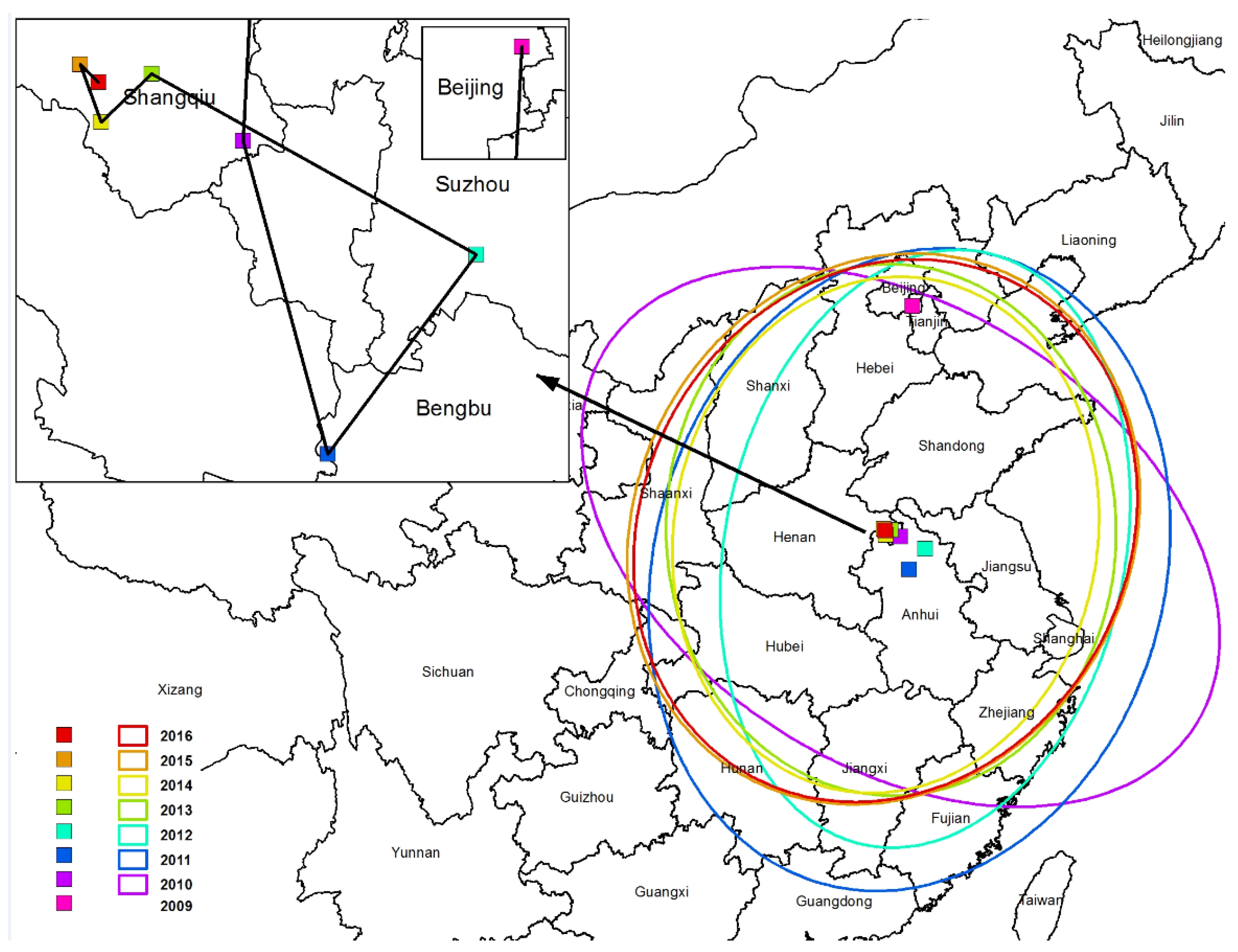
4.2. The Spatial and Temporal Evolution of Two-Star Green Residences

As observed from Figure 3, the center of gravity of two-star green residences first appeared at the junction of Beijing and Tianjin in 2009, but the weighted standard deviation ellipse began in 2010. This is because that Beijing and Tianjin became the first cities to have two-star green residences in 2009, but two points could not accurately determine the position of the ellipse.

From 2010 to 2016, the center of gravity was located in Bengbu and Suzhou in Anhui Province in 2011 and 2012, while the rest of the years were located in Shangqiu in Henan Province. The trajectory of the center of gravity can be clearly divided into a fluctuating period and a stable period. Before 2013, the center of gravity mainly shifted 1027.61 km to the south, and then moved 97.96 km to the northeast. After moving rapidly to the northwest for 140.03 km in 2013, the center of gravity began to stabilize in Shangqiu, and only moved 61.03 km in the three years.

The areas of the weighted standard deviation ellipse decreased first and then increased, which decreased from 1.99 million km² in 2010 to 1.37 million km² in 2014, and then increased to 1.69 million km² in 2016. Among them, the largest decrease and increase occurred in 2012 and 2015, when they varied by 0.56 and 0.38 million km², respectively. In 2010, the ellipse covered most of the central and eastern regions such as Shanghai, Jiangsu, Shandong, Hebei, Henan, Anhui, and Hubei, as well as some of the western regions such as Shanxi, Shaanxi and Ningxia, indicating that two-star green residences appeared in many provinces in that year. From 2011 to 2014, the ellipses gradually shrunk towards the central and eastern regions, especially in the north–south direction, which was much faster than that in the east–west direction. From 2014 to 2016, the areas of the ellipse begun to expand, and the scopes begun to expand to the western region, indicating that the two-star green residences in the western region such as Chongqing, Shaanxi and Xinjiang began to grow rapidly, but the central and eastern regions still took the lead.

The ellipse showed a spatial pattern of a northwest–southeast direction in 2010, and the rotation angle was 122.86°. This is because many provinces, including Xinjiang and Ningxia in the northwest regions, began to develop two-star green residences in 2010, and there was little difference in the number. The ellipse distribution direction approached due north and due south and the rotation angle was 178.70° due to the rapid increase in the number of two-star green residences in northern regions such as Hebei and Shandong in 2013. In other years during the study period, the ellipses made clear a spatial pattern of a northeast–southwest direction, and the rotation angle increased from 15.58° in 2011 to 29.28° in 2016.

The major axis standard deviation lessened 395.38 km from 1970.71 km in 2010 to 1575.33 km in 2016, and the minor axis standard deviation added 79.79 km from 1286.33 km in 2010 to 1366.12 km in 2016. It is obvious that the shrinkage amplitude of the major axis standard deviation is larger than the expansion amplitude of the minor axis standard deviation. Similarly, the axial ratio increased from 0.65 in 2010 to 0.87 in 2016, which also indicates that the directionality of the change trend of two-star green residence is weakening, and the weighted standard deviation ellipse gradually tended to be circular.

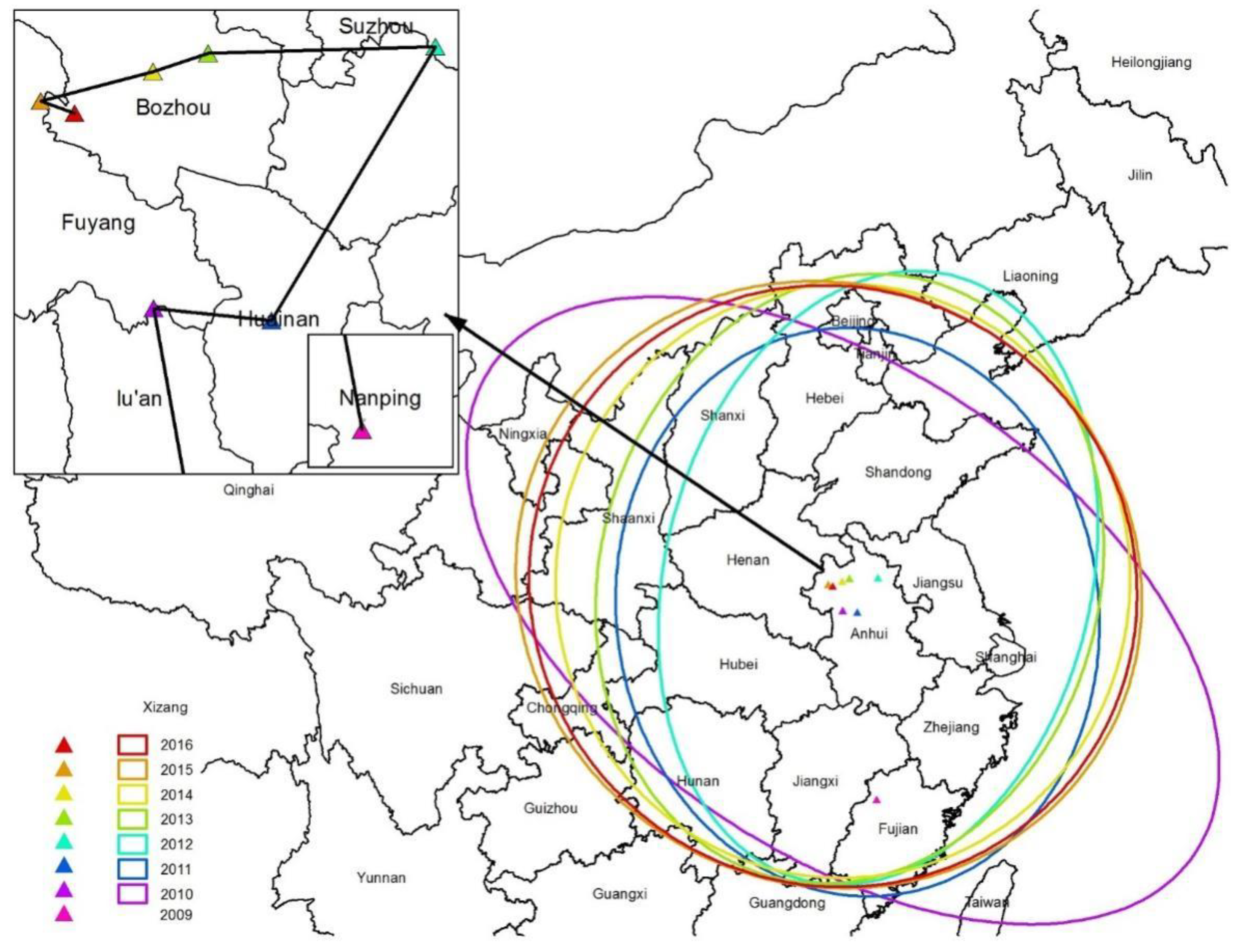
4.3. The Spatial and Temporal Evolution of Three-Star Green Residences

Prior to 2010, only two residences which were located in Shenzhen and Suzhou had received a three-star green building label. Hence, the center of gravity of three-star green residences in 2009 was located in Nanping in Jiangxi province, which is the midpoint of the two cities, and the ellipses of the three-star green residences also begun in 2010, as shown in Figure 4.

Since 2010, the centers of gravity were distributed in Anhui provinces, and the trajectory of the center of gravity moved northeast and then west in the whole. From 2010 to 2012, the centers of gravity first moved east by 54.19 km and then northeast by 157.96 km. During this period, the number of three-star green residences in Jiangsu Province was significantly higher than that in other provinces. From 2012 to 2016, the centers of gravity moved 200.67 km to the west with the rapid development of three-star green residences in the southwest and northeast provinces such as Yunnan, Guangxi, Beijing and Tianjin.

The areas of the standard deviation ellipse decreased first and then increased, which decreased from 2.78 million km² in 2010 to 1.81 million km² in 2012, and then increased to 2.49 million km² in 2016. From 2010 to 2012, the areas of the ellipse had been decreased by 0.97 million km², and the distribution range shrunk to the central and eastern regions with more favorable levels of three-star green residence development, such as in Shandong, Jiangsu, Shanghai, Zhejiang, Anhui and Henan. From 2012 to 2016, the areas of the ellipse had been increased 0.68 million km², and the scopes begun to expand to the western region, indicating that three-star green residence has developed rapidly in the western regions such as Guangxi and Xinjiang since 2013.

The distribution direction of the weighted standard deviation ellipse was northwest–southeast in 2010, 2011, 2015 and 2016, and the rotation angles were 125.00°, 172.58°, 119.38° and 125.2°, respectively. This was due to the fact that three-star green residences were mainly distributed in the southeastern coastal regions of Guangdong, Zhejiang and Jiangsu. With the vigorous development of three-star green residences in the northern regions such as Beijing and Tianjin in 2012 to 2014, the ellipses showed a spatial pattern of a northeast–southwest direction.

The major axis standard deviation shrank from 2517.72 km in 2010 to 1677.45 km in 2011, a sharp decrease of 840.27 km. After 2012, the value of the major axis standard deviation only fluctuated by 118.02 km, and the ellipse tended to be stable in the direction of the main trend. During the study period, the minor axis standard deviation increased from 1406.03 km in 2010 to 1753.6 km in 2016, an increase of 347.57 km, indicating that the ellipse had a significant expansion effect in the subtrend direction. Based on the variation trend of the standard deviation of the major and minor axes, this paper found that the axial ratio was close to one, and reached 0.97 in 2016, and the ellipse shape tended to the circle structure, indicating that the distribution direction tendency of three-star green residences was weakening.

4.4. Summary

During the research period, the development of green residences in China mainly experienced two stages: a pilot period (2008–2010) and development period (2011–2016). These pilot cities are mostly located in the central and eastern regions with relatively developed social economies, and the pilot cities of each star-rated green residence show a certain agglomeration phenomenon, such as one-star green residence first appearing in the Yangtze River Delta region, two-star in Beijing and Tianjin, and three-star in the southeast coastal area. Affected by the geographical location of the pilot cities, the weighted standard deviation ellipse of China’s green residences in the pilot period is quite different from the development period in terms of centrobaric position, direction, and scope. In the development period, China’s green residences were mainly distributed in the central and eastern regions, and the main trend of development is from northeast to southwest. In 2013, the radiation effect from the core area to the surrounding area began to appear, showing that the area of the weighted standard deviation ellipse began to increase year by year, and the center of gravity and coverage area shifted to the west obviously. With the rapid development of green residence in western region, the gap between the major and minor axes’ standard deviations is decreasing year by year, and the axial ratio is approaching one. The directionality of the development of green residence in China is gradually weakened, and the higher the evaluation level, the more obvious the performance.

5. The Driving Mechanism and Key Driving Factors of Green Residences in China

In 2019, the real estate enterprises had applied for 82% of the green building evaluation labels in China [44]. When compared with government-led policy housings, green commercial residences are more likely to be affected by external factors such as the level of urban economic and social development. Therefore, this chapter mainly studied the driving factors of green commercial residences. Due to the lack of statistics on China’s green residence marking projects after September 2016 by the CGBEL, the sample’s timeframe for this study was 2008 to 2015 due to the availability and consistency of project information.

5.1. Correlation Analysis

This paper used SPSS 26.0 software to calculate the Spearman’s correlation coefficient between the G′-scores and the 21 driving factors according to Equation (6), and the results are given in

Table 4. The results of the correlation analysis for the driving factors.

Variable	One-Star	Two-Star	Three-Star
GDP	0.651 ***	0.558 ***	0.549 ***
RGPB	0.649 ***	0.54 ***	0.6 ***
EECEP	0.511 ***	0.535 ***	0.511 ***
AQI	−0.295 ***	−0.36 ***	−0.15 ***
PRP	0.439 ***	0.442 ***	0.361 ***
UR	0.361 ***	0.362 ***	0.479 ***
UCDI	0.651 ***	0.63 ***	0.66 ***
UCHA	0.303 ***	0.339 ***	0.278 ***
PPEU	0.36 ***	0.289 ***	0.389 ***
COV	0.623 ***	0.452 ***	0.52 ***
ICR	0.603 ***	0.452 ***	0.492 ***
CRCNA	0.543 ***	0.409 ***	0.42 ***
CRCMA	0.405 ***	0.328 ***	0.308 ***
CRSA	0.482 ***	0.284 ***	0.359 ***
CRP	0.434 ***	0.38 ***	0.545 ***
CP	0.318 ***	0.244 ***	0.317 ***
EIP	0.24 ***	0.296 ***	0.141 ***
NEIP	0.176 ***	0.198 ***	0.003
DE	0.329 ***	0.34 ***	0.486 ***
GE	0.167 ***	0.293 ***	0.189 ***
CRA	0.173 ***	0.035	0.271 ***

*** represents the 1% significance level.

. The results showed a positive correlation between development of the green residences and economic growth, social development (except AQI), the real estate market, government measures, and climatic condition, and the correlation coefficients were significant at the 1% level, except that CRA and NEIP were not significant at the levels of two- and three-star green residences, respectively. This indicated that the 21 driving factors selected in this article were closely related to the green residence development and were appropriate for the following regression analysis.

5.2. Regression Analysis

Through State 16.0 software, this paper employed the panel Tobit model to quantitatively study the driving effect of the above factors on the G′-score, and further adopted the average marginal effect value to quantitatively analyze the influence of each unit change of a factor on G′-score under the condition that other factors are relatively unchanged, according to Equations (7)–(9).

Table 5. The results of the regression analysis for the driving factors.

Variable	One-Star		Two-Star		Three-Star
	(1)	(2)	(3)	(4)	(5)	(6)
GDP	8.41 ** (3.003)	2.694 *** (0.986)	−0.062 (0.959)	−0.024 (0.366)	3.921 (6.191)	0.985 (1.56)
RGPB	0.784 (1.753)	0.251 (0.562)	0.348 (0.63)	0.133 (0.241)	3.01 (3.9)	0.756 (0.981)
EECEP	0.418 (0.739)	0.134 (0.237)	0.188 (0.276)	0.072 (0.105)	−3.093 * (1.496)	−0.776 ** (0.384)
AQI	−0.278 (2.441)	−0.089 (0.782)	−0.486 (1.017)	−0.186 (0.389)	−5.713 (4.824)	−1.434 (1.215)
PRP	−8.224 ** (2.963)	−2.634 *** (0.969)	0.752 (0.949)	0.287 (0.363)	1.191 (6.04)	0.299 (1.517)
UR	0.068 (6.154)	0.022 (1.971)	3.93 (2.276)	1.501 * (0.873)	39.45 ** (14.091)	9.906 *** (3.687)
UCDI	−2.495 (3.603)	−0.799 (1.158)	4.198 ** (1.324)	1.604 *** (0.506)	8.662 (6.987)	2.175 (1.754)
UCHA	0.562 (2.316)	0.18 (0.742)	2.698 ** (0.992)	1.031 *** (0.38)	14.53 ** (5.212)	3.649 *** (1.326)
PPEU	−15.96 (13.757)	−5.111 (4.42)	−0.536 (4.328)	−0.205 (1.653)	−11.63 (29.842)	−2.921 (7.503)
COV	−0.55 (1.356)	−0.176 (0.435)	0.278 (0.408)	0.106 (0.156)	1.672 (2.719)	0.42 (0.682)
ICR	−0.941 (1.669)	−0.301 (0.536)	−0.776 (0.626)	−0.297 (0.24)	−9.137 * (3.866)	−2.294 ** (0.984)
CRCNA	0.742 (2.137)	0.238 (0.684)	−0.993 (0.784)	−0.379 (0.3)	6.311 (4.725)	1.585 (1.187)
CRCMA	−0.933 (1.019)	−0.299 (0.326)	0.306 (0.403)	0.117 (0.154)	1.65 (1.861)	0.414 (0.468)
CRSA	−0.168 (1.24)	−0.054 (0.397)	0.211 (0.537)	0.081 (0.205)	−1.062 (2.419)	−0.267 (0.608)
CRP	1.651 (2.103)	0.529 (0.677)	−0.371 (0.702)	−0.142 (0.268)	−1.549 (4.36)	−0.389 (1.096)
CP.1	1.423 (1.103)	0.488 (0.405)	−0.65 (0.505)	−0.231 (0.167)	−2.156 (1.881)	−0.511 (0.423)
EIP.1	−2.112 * (0.987)	−0.634 ** (0.281)	−0.201 (0.402)	−0.075 (0.149)	0.715 (1.878)	0.182 (0.485)
NEIP.1	3.44 ** (1.125)	1.269 *** (0.476)	0.794 (0.45)	0.327 (0.199)	0.794 (2.214)	0.203 (0.578)
DE.1	0.169 (1.151)	0.054 (0.374)	−0.365 (0.491)	−0.135 (0.175)	−2.486 (1.984)	−0.593 (0.45)
GE.1	4.063 *** (1.217)	1.531 *** (0.538)	0 (0.427)	0 (0.163)	−3.976 (2.196)	−0.916 * (0.471)
CRA.2	−1.253 (1.801)	−0.359 (0.537)	0.043 (0.543)	0.018 (0.232)	−4.296 (4.028)	−1.058 (1.078)
CRA.3	2.626 (1.976)	0.94 (0.676)	−1.122 (0.615)	−0.413 * (0.243)	−2.795 (4.231)	−0.723 (1.148)
CRA.4	−1.008 (2.722)	−0.293 (0.788)	−0.367 (0.895)	−0.149 (0.362)	2.51 (5.648)	0.775 (1.753)
CRA.5	0.303 (3.257)	0.095 (1.03)	−1.116 (1.033)	−0.411 (0.356)	1.86 (6.839)	0.562 (2.125)
_cons	−2.176 (37.819)		49.605 *** (13.964)		−208.4 ** (75.512)
σu	2.633 *** (0.552)		0.535 * (0.229)		5.858 *** (1.234)
σe	3.863 *** (0.246)		1.834 *** (0.108)		5.991 *** (0.431)
N	336		336		336
Prob (LR test)	0		0		0

Columns (1), (3), and (5) are the regression coefficients. Columns (2), (4), and (6) are the average marginal effect values. Standard errors are in parentheses. ***, **, and * represent the 1%, 5%, and 10% significance levels, respectively.

reports the results obtained from the empirical estimations.

The LR test is used to judge whether the model has individual effects. Since the p values of all the LR test results were zero, this indicated that the null hypothesis, “${\mathrm{H}}_0:{\mathsf{\sigma }}_{\mathrm{u}}=0$”, was strongly rejected. Hence, the model had significant individual effects. Because this paper could not get consistent fixed effect estimators whether using fixed effects or mixed Tobit regression [45], the random effects panel Tobit regression model was selected. The specific analysis of each influencing factor is as follows.

First, the columns one and two present the coefficients and average marginal effect values of G′-score regression results for one-star green residences, respectively. Of the 20 influencing factors (excluding climatic conditions), only 11 had a value greater than zero and played positive roles in promoting the development of green residences. The three factors with the greatest positive impact were GDP, GE, and NEIP. With other factors remaining unchanged, for each unit change in them, the corresponding G′-scores changed by 2.69, 1.53, and 1.27%, respectively. This showed that the development level of one-star green residences in cities with a relatively developed economy, introduced standards, and noneconomic incentive policy was higher than in other cities. On the contrary, for each unit of change in PPEU and PRP, the G′-scores changed by −5.11 and −2.63%, respectively. It can be considered that the educational level of residents and the number of permanent residents had significant negative impact on one-star rating. Every unit of change in the other indicators had an impact on the G′-score of less than 1%.

Second, the 20 regression parameters for the G′-score of two-star green residences had 10 positive and negative values. It is notable that only three factors (i.e., UCDI, UR, and UCHA) changed by one unit; their impact on the G′-score was greater than 1%, and their average marginal effects were 1.60, 1.50, and 1.03%, respectively. Hence, urbanization, income, and the housing conditions of residents significantly promoted two-star green residences’ development. Every unit of change in the other indicators had an impact on the G′-score of less than 0.4%, indicating that their effects on the two-star rating were weak and negligible.

Third, the numbers of positive and negative regression coefficients for three-star G′-scores were 12 and 8, respectively. The average marginal effect values of UR, UCHA, UCDI, CRCNA, GDP, and GPBR indicated that each unit of change in them increased the proportion of green residences in newly started housing by 9.91, 3.65, 2.18, 1.59, 0.99, and 0.76%, respectively. It should be noted that the influences of UR, UCHA, and UCDI on the three-star rating were much stronger than those on the two-star rating. Meanwhile, the new housing scale and economic factors also had a significant positive driving effect on the three-star rating. This paper also noticed that PPEU, ICR, and AQI had significant negative effects on the three-star green residences development, and if they increased by 1%, then the G′-stores would change by −2.92, −2.29, and −1.43%, respectively. It can be seen that the education level of residents and real estate investment could not effectively promote three-star green residential development, and cities with high air quality had insufficient motivation to develop three-star green residences.

Fourth, the climate condition was significantly correlated with green residences’ development, especially those of a three-star rating. When compared to CRA.1, the G′-store of one-star residences in the division CRA.3 increased by 0.94%, two-star in the division CRA.2 increased by 0.02%, and three-star in the divisions CRA.4 and CRA.5 changed by 0.78, and 0.56%, respectively. All others were negative. It can be seen that one-star green residences are mainly distributed in areas with hot summers and cold winters, two-star ratings are chiefly located in severe cold or cold regions, and three-star rating tend to be distributed in hot summers and warm winters, or mild areas.

By observing the regression indexes and average marginal effect values of the same factor on G′-stores with the same star ratings, this study found that there are differences in their sizes, and this difference is irregular. This proves that the development of green residences is the result of the combined action of multiple driving factors. Further comparing the influence of the same factor on G′-stores with different stars, this paper found that both the regression indexes and average marginal effect values are inconsistent in terms of sign, magnitude, and significance. This shows that the key driving factors vary between green residences with different star levels. Concretely, the economic factors played positive roles in promoting the green residences development. GDP had the strongest driving force for one-star green residences, while cities with strong economic strength also have a higher three-star green residence development index. The influence of environmental factors on green residences decreased with the improvement of evaluation grade, but the demographic factors and living standards increased with the improvement of evaluation level. Residents’ education level was negatively correlated with the development of green residences, and the change of the coefficients was not regular with the improvement of evaluation level. The city’s construction technology level and commercial housing price had different trends with the increase of green label grade. The higher the technical level of construction, the better the development of high-star green residences, but the sales price of commercial housing was just the opposite. The changing trend of the real estate market size index was not significant with the improvement of the green residence evaluation grade. Except for economic incentives, government measures showed a trend of weakening influence with the improvement of green residence evaluation level. Finally, the clusters of green residences with different star-levels had obvious climate characteristics.

6. Conclusions

With the improvement of people’s energy crisis and environmental protection awareness, green residences will become the main trend of construction industry development. However, the study on the spatial distribution characteristics of green residences and its influencing factors has not attracted enough attention in the academic circles. This paper pioneered the study of the spatial and temporal evolution of different ratings of green residences and their driving factors in China. The research results of this paper will be helpful the government to put forward targeted development plans to improve the level of local green residences, and will also be helpful real estate enterprises to make strategic decisions on green housing development.

This paper established a spatial panel database on the number of green residences with different stars owned in each city from 2008 to 2016, and a panel database on the driving factors of 42 cities with a large number of green residences during 2008 to 2015. By employing ArcGIS 10.8 software, this study calculated the SDE model parameters of each rating of green residences, and revealed the spatial and temporal evolution laws of green residences with different star levels in China at the municipal level. Through SPSS 26.0 software, the study figured out the Spearman’s correlation coefficients between the number of green residences in each star and the 21 driving factors selected in this paper, and confirmed the applicability of these factors in the research. This paper creatively introduced an improved Gini coefficient of green building development (G′-score) to represent the annual measure of green residences development in each city. With the help of Stata 16.0 software, this study took advantage of the panel Tobit model and the average marginal effect value to quantitatively analyze the driving mechanism and key influencing factors of each star-rated green residences in China from economy, society, real estate market, policy, and climate. The main conclusions are as follows.

From the perspective of evolutionary trend, green residences first appeared in economically and socially developed cities in China such as Shanghai, Beijing, Shenzhen, etc. Since 2011, China has entered a period of rapid development of green residences, and formed a relatively stable and clear temporal and spatial evolution path. The specific characteristics are as follows: the center of gravity and coverage of the standard deviation ellipse are gradually moving westward, the gap between the major and minor axes’ standard deviation is gradually narrowed, the directionality of the development trend of green residences is gradually weakened, and the evolution pattern of uniform diffusion from the core regions to the surrounding regions is gradually presented. Of course, there are differences in the specific evolution amplitude and speed of different star-levels of green residences.

From the perspective of geographical distribution, China’s green residences are mainly distributed in the economically and socially developed central and eastern regions, and the main direction layout is northeast–southwest. With the rapid development of green residences in western region, the coverage area of standard deviation ellipse gradually increased, the range expanded to the west, and the distribution shape is gradually approaching a circle. Meanwhile, the performance of especially obvious with the improvement of the evaluation level.

From the perspective of driving mechanisms, the development of green residences is the result of the interaction of various factors. Under the condition that other factors are unchanged and changed, the driving force of any factor will produce changes of increase or decrease, and this change has no rule to follow either path among different evaluation levels or among various influencing factors. Therefore, when the government formulates the local green residences development plan or the real estate enterprises make a strategic decision, it must consider the influence of various local social and economic factors.

From the perspective of key factors, the driving effect of the same factor on green residences with different star ratings is inconsistent in terms of sign, magnitude, and significance. At the same time, the driving effect of each factor under the same star rating is also different in these three aspects. For example, GDP is the most important and significant driving force for the development of one-star green residences, but the driving effect of three-star ratings has declined significantly, and even has a negative effect on two-star ratings. Similarly, the development of one-star green residences is mainly affected by the local economic level, government guidance and non-economic incentive policies, while the development of medium- and high-star ratings is mainly affected by the urbanization rate, residents’ income level and housing conditions. Therefore, the government needs to formulate differentiated green residence development plans according to the local social and economic situations. Meanwhile, developers also need to formulate targeted development strategies according to the differences in the driving factors of green residences with different stars.

The problem of “emphasizing design and neglecting operation” of green residences in China is still prominent. Due to the lack of data, this paper did not separate analyze the temporal and spatial evolution trend of green residences that have obtained operation or design markings. Meanwhile, as a kind of market behavior, the development enthusiasm of real estate enterprises and the demand of buyers are also particularly important to the development of green housing, so the conclusion of this paper may be biased. It is recommended that future studies analyze the driving factors of green residences from the perspective of internal driving mechanisms of enterprises and buyers’ willingness to pay.

References

1. IPCC. Chapter 9: Buildings. Climate Change 2014: Mitigation of Climate Change. In Contribution of Working Group III to the Fifth Assessment Report of the Intergovernmental Panel on Climate Change; Edenhofer, O., Pichs-Madruga, R., Sokona, Y., Farahani, E., Kadner, S., Seyboth, K., Adler, A., Baum, I., Brunner, S., Eickemeier, P., et al., Eds.; Cambridge University Press: Cambridge, UK; New York, NY, USA, 2014; pp. 677–678. Available online: https://www.ipcc.ch/report/ar5/wg3/ (accessed on 13 January 2022).
2. China Building Energy Consumption Research Report (2020) Released. Available online: https://cabee.org/site/content/24021.html (accessed on 3 February 2021).
3. Lian, S.H.; Liang, H. Comparative Study on Green Building Development between China and Foreign Countries. Constr. Sci. Technol. 2021, 75–80. [Google Scholar] [CrossRef]
4. Darko, A.; Zhang, C.; Chan, A.P.C. Critical analysis of green building research trend in construction journals. Habitat. Int. 2016, 57, 53–63. [Google Scholar] [CrossRef]
5. Assessment Standard for Green Building (National Standard of the People’s Republic of China, GB/T 50378-2019). Available online: http://www.mohurd.gov.cn/gongkai/fdzdgknr/tzgg/201905/20190530_240717.html (accessed on 29 August 2022).
6. Kats, G. The Costs and Financial Benefits of Green Buildings: A Report to California’s Sustainable Building Task Force 2003. Available online: http://citeseerx.ist.psu.edu/viewdoc/download;jsessionid=EE14BBCE4C2EF6E6315B38857249245D?doi=10.1.1.174.2149&rep=rep1&type=pdf (accessed on 19 October 2021).
7. Zhang, L.; Wu, J.; Liu, H. Turning green into gold: A review on the economics of green buildings. J. Clean. Prod. 2018, 172, 2234–2245. [Google Scholar] [CrossRef]
8. Wu, X.; Peng, B.; Lin, B. A dynamic life cycle carbon emission assessment on green and non-green buildings in China. Energy Build. 2017, 149, 272–281. [Google Scholar] [CrossRef]
9. Song, Y.; Li, C.; Zhou, L.; Chen, Y.; Zhang, H. Factors affecting green building development at the municipal level: A cross-sectional study in China. Energy Build. 2021, 231, 110560. [Google Scholar] [CrossRef]
10. Liu, X.; Li, P. Spatial and Temporal Evolution and Driving Mechanism of Green Building Area in China. Ecol. Econ. 2021, 37, 88–94, 142. [Google Scholar]
11. Yip, S.C.T. The Geography of Green Buildings in Chinese Cities. Mod. Urban Res. 2012, 27, 42–48. [Google Scholar]
12. Qiu, B.; Li, D.; Wu, Z. Study on the Character of Chinese Green Building Spatial Evolution. Urban Stud. 2017, 24, 1–10. [Google Scholar]
13. Zhang, L.; Wu, J.; Liu, H. Policies to enhance the drivers of green housing development in China. Energy Policy 2018, 121, 225–235. [Google Scholar] [CrossRef]
14. Choi, E.; Miller, N. Explaining LEED Concentration: Effects of Public Policy and Political Party. JOSRE 2011, 3, 91–108. [Google Scholar] [CrossRef]
15. Dippold, T.; Mutl, J.; Zietz, J. Opting for a Green Certificate: The Impact of Local Attitudes and Economic Conditions. J. Real Estate Res. 2014, 36, 435–474. [Google Scholar] [CrossRef]
16. Kaza, N.; Lester, T.W.; Rodriguez, D.A. The Spatio-temporal Clustering of Green Buildings in the United States. Urban Stud. 2013, 50, 3262–3282. [Google Scholar] [CrossRef]
17. Simons, R.A.; Choi, E.; Simons, D.M. The effect of state and city green policies on the market penetration of green commercial buildings. JOSRE 2009, 1, 139–166. [Google Scholar] [CrossRef]
18. Cidell, J.; Cope, M.A. Factors explaining the adoption and impact of LEED-based green building policies at the municipal level. J. Environ. Plan. Manag. 2014, 57, 1763–1781. [Google Scholar] [CrossRef]
19. Gao, Y.; Yang, G.; Xie, Q. Spatial-Temporal Evolution and Driving Factors of Green Building Development in China. Sustainability 2020, 12, 2773. [Google Scholar] [CrossRef]
20. Lee, T.; Koski, C. Building green: Local political leadership addressing climate change. Rev. Policy Res. 2012, 29, 605–624. [Google Scholar] [CrossRef]
21. Portney, K.E.; Cuttler, Z. The local nonprofit sector and the pursuit of sustainability in American cities: A preliminary exploration. Local Environ. 2010, 15, 323–339. [Google Scholar] [CrossRef]
22. Fuerst, F.; Kontokosta, C.; McAllister, P. Determinants of green building adoption. Environ. Plan. B Urban Anal. City Sci. 2014, 41, 551–570. [Google Scholar] [CrossRef]
23. Mason, S.G.; Marker, T.; Mirsky, R. Primary Factors Influencing Green Building in Cities in the Pacific Northwest. Public Works Manag. P 2011, 16, 157–185. [Google Scholar] [CrossRef]
24. Portnov, B.A.; Trop, T.; Svechkina, A.; Ofek, S.; Ghermandi, A. Factors affecting homebuyers’ willingness to pay green building price premium: Evidence from a nationwide survey in Israel. Build. Environ. 2018, 137, 280–291. [Google Scholar] [CrossRef]
25. Berry, S.; Davidson, K.; Saman, W. The impact of niche green developments in transforming the building sector: The case study of Lochiel Parkf Lochiel Park. Energ. Policy 2013, 62, 646–655. [Google Scholar] [CrossRef]
26. Zou, Y.; Zhao, W.; Zhong, R. The spatial distribution of green buildings in China: Regional imbalance, economic fundamentals, and policy incentives. Appl. Geogr. 2017, 88, 38–47. [Google Scholar] [CrossRef]
27. Delmas, M.; Toffel, M.W. Stakeholders and environmental management practices: An institutional framework. Bus. Strategy Environ. 2004, 13, 209–222. [Google Scholar] [CrossRef]
28. Karkanias, C.; Boemi, S.N.; Papadopoulos, A.M.; Tsoutsos, T.D.; Karagiannidis, A. Energy efficiency in the Hellenic building sector: An assessment of the restrictions and perspectives of the market. Energy Policy 2010, 38, 2776–2784. [Google Scholar] [CrossRef]
29. Franco, M.; Pawar, P.; Wu, X. Green building policies in cities: A comparative assessment and analysis. Energy Build. 2021, 231, 110561. [Google Scholar] [CrossRef]
30. Cidell, J.; Beata, A. Spatial variation among green building certification categories: Does place matter? Landsc. Urban Plan. 2009, 91, 142–151. [Google Scholar] [CrossRef]
31. Yang, X.; Zhang, J.; Zhao, J. Factors Affecting Green Residential Building Development: Social Network Analysis. Sustainability 2018, 10, 1389. [Google Scholar] [CrossRef]
32. Li, D. Regional Differences among the Development Models of Green Buildings in China—Based on statistical data from 2006 to 2014. Hous. Sci. 2019, 29, 35–43. [Google Scholar] [CrossRef]
33. Guo, K.; Yuan, Y. Geographic Distribution and Influencing Factor Analysis of Green Residential Buildings in China. Sustainability 2021, 13, 12060. [Google Scholar] [CrossRef]
34. Hao, T.; Wang, J.; Zhang, Z. Study on Spatial Evolution of Chinese Green Building. In Proceedings of the 14th International Green Building and Building Energy Conservation Conference and New Technology and Products Fair, Zhuhai, China, 2 April 2018. [Google Scholar]
35. Fu, W.; Zhou, Y. Based on ARCGIS-SDE Spatial Evolution Trend of Industrial Clusters Space. Appl. Mech. Mater. 2015, 733, 982–985. [Google Scholar] [CrossRef]
36. Du, Q.; Zhou, J.; Pan, T.; Sun, Q.; Wu, M. Relationship of carbon emissions and economic growth in China’s construction industry. J. Clean. Prod. 2015, 220, 99–109. [Google Scholar] [CrossRef]
37. Li, Q.; Zhao, Y.; Li, S.; Zhang, L. Spatial-temporal characteristics of the coupling coordination of social security and economic development in China during 2002–2018. Reg. Sustain. 2021, 2, 116–129. [Google Scholar] [CrossRef]
38. Croux, C.; Dehon, C. Influence functions of the Spearman and Kendall correlation measures. Stat. Methods Appl. 2010, 19, 497–515. [Google Scholar] [CrossRef] [Green Version]
39. Zar, J. Spearman Rank Correlation. In Encyclopedia of Biostatistics; Armitage, P., Colton, T., Eds.; John Wiley & Sons Ltd.: Hoboken, NJ, USA, 2005. [Google Scholar] [CrossRef]
40. Artusi, R.; Verderio, P.; Marubini, E. Bravais-Pearson and Spearman correlation coefficients: Meaning, test of hypothesis and confidence interval. Int. J. Biol. Markers 2002, 17, 148–151. [Google Scholar] [CrossRef]
41. Ke, Y.; Guo, J.; He, Z.; Yin, J. Research on economic evaluation of green buildings based on the correlation analysis of factors. J. Wuhan Polytech. Univ. 2016, 35, 75–81. [Google Scholar] [CrossRef]
42. Zhang, L. Study on the Driving Mechanism of Green Housing Development in Chinese Cities. Ph.D. Thesis, Tsinghua University, Beijing, China, 2018. [Google Scholar] [CrossRef]
43. Mcdonald, J.; Moffitt, F. The Uses of Tobit Analysis. Rev. Econ. Stat. 1980, 2, 318–321. [Google Scholar] [CrossRef]
44. Annual Report on Green Real Estate Development in China (2020). Available online: http://www.ugreen.cn/newsDetail/10106 (accessed on 3 February 2021).
45. Chen, Q. Advanced Econometrics and Stata Applications, 2nd ed.; Higher Education Press: Beijing, China, 2014; pp. 325–327. [Google Scholar]
Figure 1. Spatial distribution of 42 leading cities.
Applsci 12 08788 g001
Figure 2. Weighted standard deviation ellipse of one-star green residences and their center of gravity change in China (2008–2016).
Applsci 12 08788 g002
Figure 3. Weighted standard deviation ellipse of two-star green residences and their center of gravity change in China (2009–2016).
Applsci 12 08788 g003
Figure 4. Weighted standard deviation ellipse of three-star green residences and their center of gravity change in China (2009–2016).
Applsci 12 08788 g004