Featured Application
(1) Static stiffness modelling methods are classified and summarized. Each method is studied with regards to algorithms, implementation, and limitations; (2) A single degree of freedom and multiple degrees of freedom are proposed to describe the modelling methods in the joint space. (3) Regarding the relationship between external force and deformation, linear and nonlinear modelling methods are discussed.
Abstract
Due to their high flexibility, large workspace, and high repeatability, industrial robots are widely used in roughing and semifinishing fields. However, their low machining accuracy and low stability limit further development of industrial robots in the machining field, with low stiffness being the most significant factor. The stiffness of industrial robots is affected by the joint deformation, transmission mechanism, friction, environment, and coupling of these factors. Moreover, the stiffness of a robot has a nonlinear distribution throughout the workspace, and external forces during processing cause irregular deviations of the robot, thereby affecting the machining accuracy and surface quality of the workpiece. Many scholars have researched identifying the stiffness of industrial robots and have proposed methods for improving the performance of industrial robots, mainly by optimizing the body structure of the robot and compensating for deformation errors with stiffness models. This paper reviews recent research on the stiffness modelling of industrial robots, which can be broadly classified as finite element analysis (FEA), matrix structure analysis (MSA), and virtual joint modelling (VJM) methods. Each method is studied from three aspects: algorithms, implementation, and limitations. In addition, common measurement techniques have been introduced for measuring deformation. Further research directions are also discussed.
Keywords:
robotic machining; position compensation; stiffness modelling; FEA; MSA; VJM; deformation measuring 1. Introduction
Since precision has improved and manufacturing costs have decreased, robots have been widely adopted in different industrial fields. Compared to computer numerical control (CNC) machine tools, industrial robots have a low cost, high flexibility, and large workspace, and they have gradually become popular in the manufacturing industry. An industrial robot can replace traditional CNC machine tools to complete part of a machining task [1,2]. At present, industrial robots can perform primary machining processes, including milling, drilling, grinding, cutting, deburring, polishing, and friction stir welding [3,4]. Industrial robots are used in industries such as aerospace, automobile manufacturing, casting, medical treatment, plastics, and wood processing [5,6,7,8]. Especially for machining large-scale components, e.g., drilling holes on the inboard flaps [9] and milling operations for windmills [7], industrial robots are more efficient than machine tools. Machining is an important process from raw materials to finished products [10] that is mainly realized using machine tools with high precision and stability. Although industrial robots have advantages, their low stiffness characteristics can cause unexpected deformations and vibration/chatter during the machining process [11,12]. Two types of industrial robots, parallel robots and serial robots, are being investigated for machining. A parallel robot is a type of closed-loop structure (Figure 1a), which is composed of a mobile platform connected to a fixed base by a set of identical or different parallel kinematic chains (legs) [13]. A serial robot is a type of open-loop structure, as shown in Figure 1b. It is constituted by a mechanical system consisting of robust links (arms) coupled with either rotational or translating joints. Different tools can be fixed on the flange for machining tasks. Due to the closed-loop structure, the parallel robot has the characteristics of high stiffness and position accuracy compared to the serial robot. However, this structure limits the robot’s operational workspace and flexibility. As a result, more research has been conducted to improve the stiffness of the serial robot. In the machining process, a cutting force of 500 N introduces a position error of 1 mm to a serial robot, while the error introduced to a CNC machine tool is less than 0.01 mm [4,14,15]. The experimental results indicate that the static stiffness of industrial serial robots is in the range of [16,17,18]. In addition, the stiffness changes as the robot’s posture configuration changes, resulting in a nonlinear distribution throughout the workspace, which leads to inaccurate machining [19]. Therefore, most industrial robots operate in fields with low precision requirements and no external contact forces. The number of industrial robots in high-value-added, high-precision industries is far lower than the number of CNC machine tools.
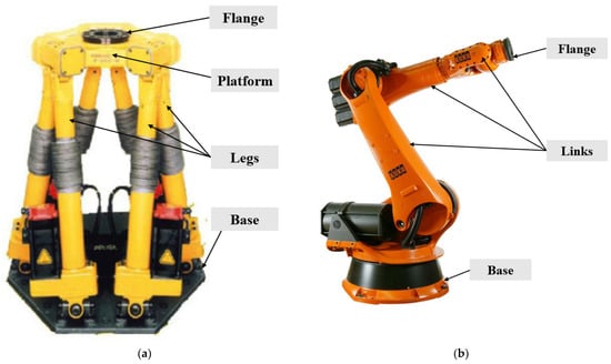
Figure 1.
Two types of industrial robots for the machining process: (a) a hexapod parallel robot and (b) a KUKA six-axis serial robot.
The stiffness of industrial robots depends on a variety of factors. The primary sources are elastic deformation caused by the geometric and material properties of various parts, including the joints, connecting links, bases, actuators, and other transmission components of robots. Furthermore, the active stiffness provided by the position control system of robots requires consideration [20,21,22,23]. Joint deformation results in most errors. Under the weight or wrench of a robotic arm, an additional angle increment is generated by the joint deformation. Then, the angle increment multiplied by the long-length mechanical arm would result in serious errors in the end effector (EE) and reduce the precision and machining quality. Therefore, traditional research usually ignores other deformations and focuses solely on joint deformation.
Nevertheless, for many engineering applications, other deformation factors cannot be ignored, such as heavy load conditions, hard material removal, and high-temperature operations [24,25,26,27,28].
- To improve the stiffness of a robot, manufacturers typically increase the cross-sectional area of the arm, which increases the weight of the robot. In addition, large-part production requires the use of large robots. Due to the gravity of the connecting link and the high load on the EE, each joint of the robot has a large deflection, and the running trajectory of the EE has a large deviation [27,29,30].
- Significant variation in robot stiffness affects the stability of the machining process. In this case, machining chattering problems are particularly prominent [6,31,32,33].
- High temperatures usually cause thermal deformation and expansion in robot parts. Model parameter errors can occur during the stiffness identification process [28].
This paper summarizes the development and application status of industrial robots, as well as the challenges that industrial robots face during machining processing. It provides a comprehensive review of robot stiffness research. The remainder of this paper is structured as follows. Section 2 introduces methods for improving the stiffness of industrial robots. Section 3, Section 4 and Section 5 introduce in detail the FEA, MSA, and VJM research results and deformation measurement, respectively. In Section 6, the common measuring techniques are introduced for measuring the deformation. Section 7 summarizes the research results and proposes future outlooks.
2. Methods for Improving Robot Processing Accuracy
To improve the accuracy of robotic machining, two main approaches are being studied to overcome the above problems. The first approach is optimizing the structure of industrial robots to improve their inherent stiffness properties. Fang et al. developed a new type of industrial robot and improved its stiffness using a hybrid structural design with open-loop and closed-loop motion chains [34]. Specialized end-effectors, such as antennas and pressure feet, were designed to improve the machining stability and stiffness of the robot during drilling and boring operations [35,36].
Manufacturers of industrial robots have also optimized the mechanism design so industrial robots meet the stiffness requirements of production processing. For example, ABB produced IRB 6660 for press tending and machining, which has an additional parallel arm to increase the stiffness of the robot and a special dual-bearing design to overcome the fluctuating process forces during machining [37]. KUKA offered KR 500 FORTEC MT (machining tooling), which was designed for high-payload milling applications [38]. In addition, some researchers have proposed improving the structural stiffness of robots by optimizing the materials used for robot joints and manipulator arms [39,40,41].
The second approach is to compensate for deformation during processing with a static stiffness model. The principle of compensation control is shown in Figure 2. First, an external force is acquired and transformed with sensors installed on industrial robots. When combined with the transformed data and joint angles directly acquired from the robot system, the stiffness model outputs the deformation after calculation to calibrate the robot [23]. In general, robot stiffness parameters are not provided by the manufacturers of industrial robots. For this reason, a stiffness model must be developed using dedicated experimental research [42].
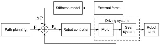
Figure 2.
Schematic diagram of deformation compensation.
The stages of compensation execution can be divided into online compensation and offline compensation, with the main difference being whether the error model input needs to be obtained online.
Model-based online error compensation relies on the acquisition of the actual position of a robot, which includes the 3D/6D Cartesian coordinates of the robot tool central point (TCP) or each joint angle. The TCP position is normally measured using optical metrology equipment such as a laser tracker, coordinate measurement machine (CMM), and 3D camera systems [43,44,45]. The joint angle is measured using a secondary encoder mounted at the output of each joint [9]. Then, real-time compensation is carried out based on the errors between the actual and theoretical coordinates [25,27,46,47,48,49,50]. Since the measurement accuracy of the metrology equipment is much higher than the positioning accuracy of robots, this method has the advantage of high precision. At the same time, some scholars combine the algorithm model with the stiffness evaluation to improve the accuracy of the stiffness evaluation [51,52], including the controller strategy, recursive algorithm, etc. For example, Flacco et al. combined a residual-based estimator of the torque at flexible transmission and a recursive least squares stiffness estimator based on a parametric model to conduct an online stiffness evaluation. Without a joint torque sensor and speed measurement, this method exhibits good robustness [53]. However, it also presents the following problems [54,55,56]:
- Online error compensation is difficult to implement, has high hardware requirements, high sensor costs, and a long operating time.
- Sensors have some inherent limitations in the application process due to sensor data noise, communication delays between the sensor and the robot controller, and the interference suppression bandwidth of the robot EE.
- The measurement system is susceptible to external factors, which greatly reduce the measurement accuracy. For example, a chip generated by cutting hinders the real-time measurement of the optical measurement system.
Compared with online error compensation, model-based offline compensation requires less auxiliary hardware. Therefore, it reduces the costs and maintains the flexibility of the robot [57,58]. At present, the main methods for robot stiffness modelling are FEA, MSA, and VJM [21,59,60,61,62,63,64,65,66].
Due to its high precision and high computational cost, FEA is used in the structural design stage. MSA simplifies the robot’s structure but reduces the modelling accuracy [67]. Moreover, FEA and MSA focus on structural design and stiffness performance analysis. VJM adds virtual axes to traditional rigid-body modelling to describe the deformation of key structures, manipulators, drive motors, and transmission structures, resulting in a reasonable balance between model accuracy and computational complexity that has been widely applied in industrial fields [68,69,70]. The static Cartesian stiffness of a robot in a workspace and at different postures can be determined by studying stiffness models. Different types of performance indicators have been introduced to evaluate the stiffness of robots [71,72,73,74,75,76], including the Jacobian eigenvalue, norm index, operability index, isotropic compliance property, and stiffness ellipse. Some scholars have compared and evaluated some stiffness performance indicators, which is convenient for selecting the corresponding indicators [77]. For milling, grinding, drilling, and spraying, redundant axes expand the workspace and provide greater flexibility for trajectory optimization [78,79]. In the following sections, the FEA, MSA, and VJM stiffness modelling methods and relevant research results are introduced.
3. FEA
FEA is considered to be an accurate method for modelling robot stiffness [62,63]. Due to multidimensional deformations, additional degrees of freedom (DOFs) are introduced into the robot system. Therefore, the FEA method is used to divide a continuous body with infinite DOFs into a specific number of flexible elements with mass and stiffness characteristics, reducing the problem to a structural problem suitable for numerical solutions. Moreover, based on the invariable mechanical properties, a certain distribution relation can be established for the displacement of the elements, the dynamics equations of the elements can be derived, and the dynamics equation of the robot system can finally be obtained through the element group [80]. A schematic diagram of a robot processed by the FEA method is shown in Figure 3.
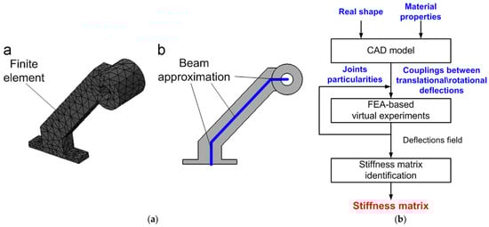
Figure 3.
Stiffness identification with FEA [59]: (a) CAD model of a link with a complex shape and (b) algorithm for the stiffness matrix identification procedure.
In FEA modelling, the accuracy of the analysis depends on the design of the CAD model, the boundary conditions of the parts, and the parameter settings of the simulation. A specific discussion of these three factors is as follows [31]:
- A well-designed robot CAD model can improve the accuracy and calculation efficiency of the stiffness model. First, a 3D geometric model of each manipulator is established. Then, the transmission components, such as the bearings, motors, and gears, are removed. Mass units are used to replace the matching in each robot joint. This process simplifies the robot joint fit and reduces the calculation. Additionally, parts and features that have little influence on the stiffness of the robot, such as the pinhole and fillet of the non-bearing parts and rounded corners, are simplified.
- The material properties, including the material of the mechanical arm and the type of heat-treatment process, are specific to the CAD model parts of the robot.
- The parameter settings of the simulation model affect the complexity, calculation speed, and accuracy of the system modelling. Generally, reasonable mesh cell type, mesh density, and mesh quality settings not only save calculation costs but also maintain calculation accuracy.
Starting with a simple beam model and ignoring complex shapes, Corradini et al. established a stiffness model of the H4 parallel robot using the FEA method. In good agreement with the experimental measurement, FEA was used as an effective and accurate tool for obtaining the mechanical parameters of the robot [81]. Bouzgarrou et al. used CAD models of each mechanical leg, added link parts and defined each rotary joint, and then established an FEA model of the parallel platform mechanism T3R1. Based on this model, the static stiffness of the robot was calculated and represented in the whole workspace [82]. Pashkevich et al. introduced a local 6-DOF virtual spring to replace the flexibility of a connecting link and used FEA modelling to determine the high-precision stiffness parameters of the spring. In their experiment, they added auxiliary objects to the CAD model of each link as a reference to evaluate the compliance of the link. In addition, unlike FEA modelling of the entire manipulator, this method only evaluated a single link at a time, which greatly reduced the FEA calculation cost [83]. Furthermore, Klimchik et al. proposed a method for obtaining the stiffness parameters of the manipulator. Each robot connecting link was modelled using the FEA method. During the modelling process, the CAD model considered six parameters: the shape, cross-section, material distribution, physical properties of the connecting link, specificity of the connecting link joints, and coupling of translational/rotational deflection. In addition, the method reduced the error of FEA modelling. The reason for this is that additional random error was assumed in the “stiffness transformation”, and the abnormal values of the experimental data were eliminated. Based on experiments using the Orthoglide series-parallel manipulator, the accuracy of this model reached 0.1% when using a 2 mm parabolic mesh, and the test force and test moment were 1 and 1 , respectively [59].
In addition to directly applying the FEA method in robot stiffness modelling, it can be used to prove the validity of other models. In [21,62,64,84,85,86,87], the FEA method was used to verify the accuracy of the MSA method, while in [29], it was used to verify a VJM model. More complex models can also be verified using FEA [88,89].
The FEA method has unique limitations. As the number of finite elements increases, the continuous calculation of mesh nodes has higher requirements for computer hardware, the calculation time increases, and calculating the inversion of high-dimension matrices becomes increasingly critical [59,62].
4. MSA
The MSA method is a common technical method in the machinery industry. When analysed from the perspective of structural mechanics, a link of a robot can be regarded as a single beam structural unit (Figure 4). It assumes that the materials and structures of the links have perfectly linear behaviour, and dynamical effects are negligible. The deformation at the free end under an external load (force/torque) can be defined as (1).
where K is the stiffness matrix. is a 6-dimensional deformation vector including three translational displacements and three rotational angles . Correspondingly, the external load W is also a six-dimensional vector containing the force and torque . For typical beams with regular cross-sections, the stiffness matrix K can be calculated analytically with information on the beam properties (beam cross-section area and Young’s modulus and shear modulus of the beam material). When beam units are combined by joints to build a robot structure, the stiffness matrix K can be obtained based on the static equilibrium of the structure. Furthermore, joint link inertia and transverse and axial deformations must be considered [62]. Subsequently, considering the rotation matrix and boundary condition constraints between each beam unit, the local stiffness matrices can be assembled into a global stiffness matrix for the robot [90,91,92]. Based on the existing research results and the characteristics of the MSA method, it has been widely used in the stiffness modelling of parallel robots.
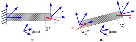
Figure 4.
Deflections and wrenches of beam structural units [63]: (a) cantilever beam and (b) unsupported beam.
Clinton et al. used the MSA method to model the stiffness of the Stewart parallel robot for the first time. Two assumptions were made in the experiments. First, the connecting links of the robot were only subjected to tensile deformation without bending. The second was that the stiffness of the robot frame was much stronger than that of the connecting link. The experimental results demonstrated the effectiveness of the MSA method for stiffness modelling [93]. For further study, Goncalves et al. first obtained the stiffness matrix of a 6-RSS parallel robot by considering the stiffness characteristics of elements such as the connecting links, actuators, and joints. Additionally, the stiffness of the joints and brakes were ignored by this simplified model [21]. To investigate the influence of joint stiffness, Deblaise et al. established two PKM stiffness models based on MSA. The first model assumed that the robot’s joints were rigid and only considered the deformation of the connecting links, while the second model considered the deformation of both the robot’s connecting links and joints. Load experiments showed that the second model was closer to the true elastic deformation of the robot [63]. Azulay et al. also considered the flexibility of the robot’s connecting links and joints. The MSA method was applied to derive a high-precision static stiffness model of a 9-DOF redundant and reconfigurable 3 × PPPRS parallel mechanism [91]. Based on the assumption of 12 DOFs for each link (Figure 5), Shi et al. proposed an MSA model of a complex EAST Articulated Maintenance Arm (EAMA). The model matrix was simplified based on boundary constraints. Compared with the FEA method, the prediction error of this method was less than 5%, which is within the acceptable prediction error range, and the computational efficiency was improved [87].
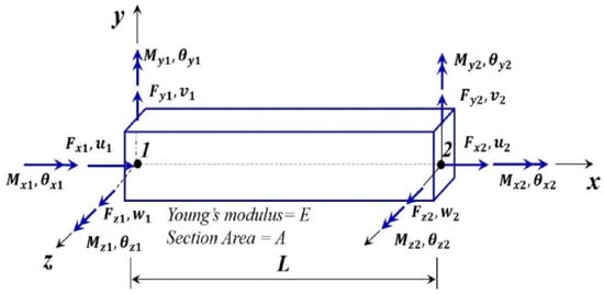
Figure 5.
12-DOF beam element in MSA method [87].
For different types of connections, the stiffness matrix can be different. In Figure 6, rigid and elastic connections are used in the two-link serial system. A Cartesian stiffness matrix for rigid connection can be deduced. This matrix is non-singular and invertible. When the connection is elastic, the Cartesian stiffness matrix is rank-deficient and singular. To efficiently apply the MSA method to serial and parallel robots, Klimchik et al. [63] developed an approach to model robot stiffness with a set of two groups of matrix equations describing the elasticity of separate links and connections between links. The general components and structures in a robot were modelled with this approach. A three-degrees-of-freedom planar parallel manipulator was selected for demonstration. The proposed MSA-based approach was approved to be in good agreement with FEA modelling. A level of 10 ms of computational efficiency can be achieved for stiffness modelling per manipulator configuration.
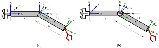
Figure 6.
Two types of connections in a two-link serial system [63]: (a) a rigid connection and (b) an elastic connection.
Detert et al. viewed the original MSA elements as having a limitation that could be entirely represented by beam theory. Therefore, an extended program was developed to automatically calculate the global stiffness matrix and deformation in a given structure composed of different elements under external loads. In this method, the nonlinear stiffness of the complex joints, links, and rolling contact bearings were all considered. The nonlinear stiffness characteristics were explained through several iterations of the linear model. After conducting experiments on the reconfigurable modular multiarm robot system PARAGRIP, their model demonstrated effective deformation prediction in the X, Y, and Z directions. The Z-direction had the best prediction effect, which can be used to compensate for robot errors due to gravity [65]. Lu et al. introduced a dynamic external load and inertial external wrench into the overall stiffness model of a parallel robot [94].
Moreover, some scholars have applied the MSA method to model the stiffness of serial robots. Kefer et al. proposed nonlinear flexible stiffness modelling of 6-DOF serial robots based on the MSA method, which achieved comparable accuracy to the FEA method. The model considered the flexible connecting link and the nonlinear characteristics of the joints as the posture changed. Finally, an energy index (2) was introduced to evaluate the precision of the model, with and representing the induced force vector or wrench and the corresponding displacement vector, respectively. Compared with the FEA method, the deformation energy index was less than 0.03% in the whole workspace. In addition, the calculation time was greatly reduced. However, actual measurement experiments were not performed, and the model was only applicable for robot error predictions in stationary states [62].
Compared with the FEA method, the MSA method has clear advantages when used with large flexible components. Many component elements are simplified to some degree, which effectively reduces the calculation cost and achieves a reasonable balance between calculation time and accuracy [83,84]. Unlike the VJM method, the MSA method does not use differential equations. Therefore, when describing the complex structure of a robot with a large number of closed loops and crosslinks, the MSA method reduces the complexity of the calculation [95]. However, more details need to be considered in MSA models, such as the nontrivial actions of the passive and elastic joints [63].
5. VJM
The traditional VJM method first defines each joint of a robot as a virtual spring and assumes that the connecting link has no deformation (Figure 7). It establishes a rotational stiffness matrix for the robot joint space. The Cartesian stiffness is calculated based on the transformation of the kinematic Jacobian matrix . The mapping relation of the stiffness matrix in Cartesian space to joint space (3) was first proposed by Salisbury [68] and has been applied in the industry [42,72,90].
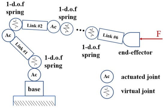
Figure 7.
Schematic diagram of the serial robot with the VJM method.
To improve the accuracy of stiffness prediction based on the traditional VJM method, researchers have considered the working conditions of various industrial robots and further developed the VJM method. The stiffness of an industrial robot is affected by various factors, including joint flexibility, link flexibility, and transmission structure flexibility. To some extent, each factor can be defined as a DOF in robot joint stiffness research. This paper divides the research into single-DOF and multiple-DOF stiffness models and describes them in detail.
5.1. Single DOF
The most commonly used and simplest stiffness modelling method is single-DOF VJM modelling. As mentioned above, joint deformation is the most significant of the various deformations. Many studies on the joint stiffness of a robot with a single DOF focus on joint deformation. The torque of the corresponding joint is required in the model. However, different measurement methods have revealed different accuracies for torque measurements under joint deformation.
The majority of researchers use force analysis to approximate joint torque. According to the static equilibrium equation, wrenches on an EE can be decomposed to calculate the torque of each joint [29]. Some scholars calculate the torque of a joint by obtaining the motor current corresponding to each joint. The reason for this is that each joint of an industrial robot is driven by an independent drive motor due to the reducer and transmission structure [96,97,98]. However, deriving the torque from the motor current usually gives inaccurate results.
The single-DOF joint stiffness model can be divided into linear stiffness and nonlinear stiffness based on the characteristics of the hypothetical virtual springs.
5.1.1. Linear Stiffness
Linear stiffness simplifies the elastic deformation of each joint to a constant joint rotational stiffness coefficient. Therefore, in Equation (2) is a diagonal matrix and each joint stiffness coefficient in the matrix is a constant.
Pan et al. adopted this method to establish a stiffness model for the ABB IRB6400 robot. The measurement position was defined in the working space. After loading the motor spindle at the end of the robot, the 3D displacement and 6D wrench data were measured. In addition to these data, the stiffness of each axis joint was calculated using the least squares method, and an end-milling experiment on the cylinder head was carried out. The real-time deformation compensation based on the stiffness model was effectively reduced from the original surface dimensional accuracy of 0.9 mm to 0.3 mm [99,100]. Eberhard Abele et al. [101] used two methods to obtain the Cartesian stiffness distribution of a five-joint industrial robot. The first method directly measured the stiffness of each joint. When measuring one joint, the other joints were fixed to prevent a coupling effect between all the joints. With Equation (3), the Cartesian stiffness was calculated using a rotational stiffness model. The second method was to directly measure the stiffness of the robot end. Four 800 mm × 800 mm planes were selected in the Z-direction of the robot coordinate system (Figure 8), and 16 positions on each plane were selected to measure the X, Y, and Z stiffnesses of the robot EE. The stiffness of the entire plane was fitted through cubic interpolation. The experiment indicated that the second method estimated the stiffness better. The main reason was that the first method approximated the joint as a linear torsion spring. This stiffness estimation introduced errors due to other deformations. The second method, which directly measured the stiffness of the end, considered the deformation of the whole joint and the robot links [102]. Subsequently, this method was applied to model the stiffness of five-axis robots and PA-10 seven-axis robots, achieving good results in error compensation. However, this method requires a large quantity of experimental data, and the nonlinear difference estimation of the unmeasured position introduces certain errors [103,104].
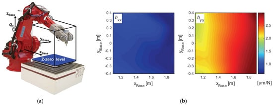
Figure 8.
Experimental setup and result [102]: (a) Focused work space and Z-level. (b) Experimental direct−compliance hxx in the X-direction and hyy in the Y-direction.
A further study on the traditional VJM method was conducted by Shih-Feng Chen and Imin Kao. They found that the traditional method included a nonconservative transformation, and (3) was used on a robot without an external load. Therefore, based on the traditional method, a supplementary stiffness matrix:
Equation (4) was introduced to describe the structural change caused by the external load on the robot EE, where is the ith joint angle and is an column vector, with and i is the number of the joint. Therefore, is an matrix. Besides, as shown in (5):
A conservative congruence transformation (CCT) was proposed between the rotational stiffness and Cartesian stiffness of the robot. Based on a digital simulation of the double-link planar manipulator, the work of the robot in the Cartesian space and the joint space was calculated. The results indicated that the CCT method was closer to the actual situation than the traditional method [70,105,106]. Gürsel Alici and Bijan Shirinzadeh used experimental methods to calculate the axis joint stiffness and Cartesian stiffness of a six-axis continuous articulated robot, further verifying the effectiveness of the CCT method [107].
Based on the CCT method, Dumas et al. identified the rotational stiffness of the KUKA KR240-2 robot. The effect of the supplementary stiffness matrix on was analysed. It was found that the larger the torque applied to the robot EE, the greater the effect of on . Therefore, when EE is subjected to a large force and torque, the stiffness of the robot will have a large deviation from the actual situation. At a specific location, however, could be ignored relative to . For this reason, the conditional number based on the Frobenius norm (6):
was defined to identify and determine the measuring position where the effect of on could be ignored [72,108]. Therefore, Equation (7) let become a standard Jacobian matrix:
is a identity matrix and is a zero matrix. Moreover, is the characteristic length, obtained by means of the methodology proposed in [16], and it normalizes the units in the Jacobian matrix. Then, the inverse condition number of is illustrated in Figure 9 [72]. The lower is, the closer the robot is to singularities. As the robot pose is close to the singularity, the determinant of approaches zero, which leads to abnormally high Cartesian stiffness . Therefore, the VJM method is not suitable for the estimation of the Cartesian stiffness near the singular position [109].
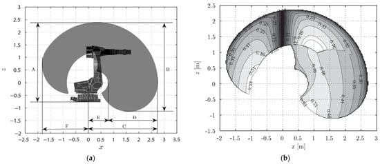
Figure 9.
Distribution of the inverse condition number in the Cartesian workspace of a KUKA robot [109]: (a) Cartesian workspace of the KUKA KR240−2 robot and (b) contours of the inverse condition number of .
By applying the CCT method and using Equation (4), Yang et al. identified the rotational stiffness of a robot in the entire workspace. The results of the study indicated that the effect of on was greater than 10% in a small part of the workspace, whereas its effect in the rest of the workspace was less than 5%. This result was consistent with Dumas’s conclusion [98]. Huseyin Celikag et al. also used the CCT method to establish a stiffness model of the ABB IRB 6640 robot and applied the model to milling processing. Given the characteristics of milling, only five DOFs were necessary to satisfy the positioning requirement. Hence, the DOF of rotation about the tool axis became functionally redundant. Due to the redundant DOF, the robot’s posture can be changed without changing its position. In the milling experiment, the 2D plane of the working space was evenly divided into positions 1 cm apart. While keeping the direction of the tool axis unchanged, the tool axis was planned in 0.01 rad increments in the interval (0, 2π). Based on the stiffness model, the stiffness of each robot posture was identified. According to a comparative analysis, the change rate of the robot Cartesian stiffness at each position in the working plane was between 58% and 161% [19]. For a six-DOF industrial robot, in general, the first three joints determine the robot’s position in joint space, while the last three joints determine the robot’s posture. Ambiehl et al. defined the first three joints as arm joints and the last three joints as wrist joints. In their research, two bottlenecks were observed. First, the stiffness value of each arm joint was 10 times greater than the stiffness value of each wrist joint. This ratio was too high to cause joint stiffness identification errors. In addition, with and without loading, the translational/rotational deflection was not homogeneous. To resolve this issue, a decoupled partial pose method (DPP) was proposed based on a metrological measurement. After “flange transformation” proposed by Ambiehl, the load variability shifted to the centre of the wrist. Using experiments on a dual-encoding industrial robot, the DDP method achieved 84% deflection error compensation under local posture decoupling [110]. Due to the effectiveness and convenience of the CCT method, it is widely used in single-DOF VJMs [17,20,75,111,112,113,114,115,116].
5.1.2. Nonlinear Stiffness
In contrast with linear stiffness models, the joint rotational stiffness coefficients in nonlinear stiffness models are not constant. In a nonlinear stiffness model, each joint stiffness coefficient in the matrix changes with the joint angle. The joint stiffness exhibits nonlinearity, which is more realistic.
Schneider et al. identified the stiffness of the six DOFs of industrial robot joints and displayed the nonlinear characteristics of the joint. First, force and torque sensors were installed on the end flange of the robot. Wrenches on the robot EE were measured from the maximum load in the negative direction to the maximum load in the positive direction. An optical measurement system was used to detect the 6-DOF deformation of each joint in the loaded and unloaded states. The distribution diagram of the rotational stiffness of joint four based on the measurements of four different positions and postures is shown in Figure 10a. The stiffness identification results demonstrated that (i) the amplitude of the displacement deformation in the X, Y, and Z directions was within the measured noise range, and there was no clear trend change; and (ii) the joint deformation was mainly rotation angle deformation. The torques in the X- and Y-directions had linear relationships with the torsional deformation in the X- and Y-directions, while the torque in the Z-direction had an approximate cubic relationship with the torsional deformation in the Z-direction. The rotational stiffness of the six joints is shown in Figure 10b. Therefore, the nonlinear least squares method was used to fit the rotational stiffness data and establish a stiffness model. Through static wrench loading, the position of the robot EE in the Cartesian coordinate system was measured. The error between the predicted value and the measured value based on the stiffness model was less than 36%. Moreover, there was no model compensation delay. To better verify the performance of the model, a machining experiment was carried out to mill a circle with a diameter of 70 mm on a steel workpiece. Comparing the milling performance with and without stiffness compensation, the absolute average position deviation was reduced from 0.39 mm to 0.2 mm [117,118].
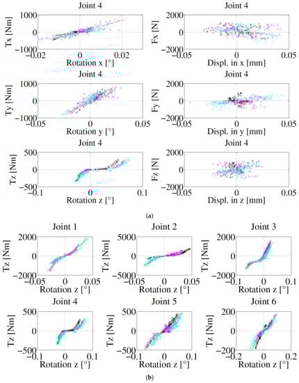
Figure 10.
Diagram of the joint deformation distribution [117]: (a) 6D stiffness model of joint four and (b) rotational stiffness around the Z-axis of each joint. Four configurations are indicated by different colors in figure and lines are the result of linear least square fitting of experimental measurement data.
5.2. Multiple DOFs
Due to the flexibility of the joints, other factors can be introduced to develop multiple-DOF VJM stiffness models.
5.2.1. Three DOFs
A three-DOF VJM not only considers the joint deformation but also introduces two additional deformations to the stiffness model. Abele et al. proposed a modified stiffness modelling method. In addition to the joint deformation, both the bearing tilt stiffness and the deformation of the connecting link were considered, as shown in Figure 11. With this method, each joint was increased from a single DOF to three DOFs. With the D-H method, the abovementioned model of the robot was increased to 15 DOFs, and the Cartesian stiffness value was calculated using Equation (2). Compared with the basic stiffness model, the predicted value of the modified stiffness model was closer to the actual measured value. The maximum error was less than 30% [101].
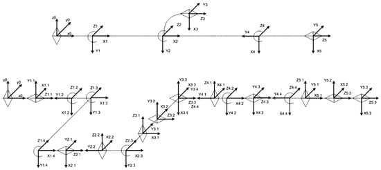
Figure 11.
Three DOFs stiffness model in [101].
5.2.2. Six DOFs
Klimchik et al. considered the deformation of all components for stiffness identification. Each driving joint and connecting link were described by a 6 × 6 stiffness matrix. Hence, 258 parameters were used for a traditional 6-axis robot. To solve this hypothetical model, a simplified model was proposed to reduce the number of identification parameters while maintaining the accuracy of the stiffness model identification [66]. In further research, Klimchik et al. introduced the gravity G of a robot arm and an external load F into stiffness modelling (Figure 12). The relationship between the wrench and the displacement of the robot EE was linearized. Based on the static balance equation, the Cartesian stiffness was calculated. When this model was applied for deformation compensation control during the robot milling process, the static deviation was effectively improved [119].
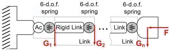
Figure 12.
VJM of an industrial robot with auxiliary loading [120].
In the general case, the stiffness matrix can be expressed by (8), with Hessian expressed using (9). A small change in the Jacobian matrix of the robot is expressed by its second derivative . Similarly, a slight change in the gravity load G is represented by its first derivative . Among them, and are expressed in (9) and (11) [119].
Based on this stiffness model, Klimchik et al. further analysed the structure of a gravity compensator in heavy industrial robots. A gravity compensator was attached to joint 1 and joint 2 and formed a closed loop, which was defined as a linear spring structure and generated torque at joint 2. Combined with the stiffness of joint 2, the stiffness of the compensator was transferred to joint 2 to determine the equivalent stiffness of this joint. Thereafter, the geometric parameters of the compensator and the rotational stiffness were identified through experiments [30,42]. Before and after loading, the deformation data of each joint were directly read by a secondary angle encoder [121], and a rotational stiffness model was established based on these data. Finally, three methods for position compensation feedback control were established, which used information from a single-angle encoder, a double-angle encoder, and a modified stiffness model. The analysis found that compared with traditional robot feedback control (angle feedback from the main angle encoder), the modified stiffness model effectively improved the position accuracy of the robot. The deformation error was reduced by more than 80%. However, the model was complex and computationally intensive. Therefore, the numerical iteration process of the static equilibrium structure took a long time to converge. For heavy industrial robots with gravity compensators, Peng Xu et al. proposed an efficient stiffness model. This model processed each joint/link as a virtual spring with six DOFs. In the model, all kinds of deformation were considered, including joint/link flexibility, link weights, and gravity compensators. First, the expressions for the reaction forces of each joint were derived from joint 6 to joint 1 for static equilibrium. Then, a stiffness model was established in conjunction with the CAD model and FEA method. An experiment on the deformation of the KUKA KR 500 industrial robot (KUKA, Augsburg, Germany) was used to verify the correctness of the model. The theoretical value of the model was close to the measured value when an external load was added to links 4 and 5. Furthermore, when the first and second derivatives decreased, the computation time of the model was greatly reduced. In addition, EE deformation, which is caused by different factors, including the external wrench, gravity compensator, and link weights, can be separated under certain conditions [29].
6. Deflection Measurement
Normally, external loads (such as mass in Figure 13) would be exerted on the robot EE to bring about the deformation. The measurement technique has a significant influence on the parameter identification and selection of the stiffness modelling method. Several techniques can be used to measure deformation, including laser trackers, optical CMMs, laser interferometers, and digital image correlation (DIC) techniques [122]. The common equipment for deformation measurement in robot stiffness modelling contains a laser tracker and optical CMM [123], which are described in detail as follows.
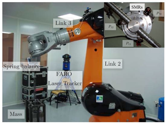
Figure 13.
Experimental setup for deformation measurement with laser tracker [109].
6.1. Laser Tracker
The laser tracker is most commonly used for tracking the robot’s EE position. It projects a laser beam onto an optical target that is in contact with an object to be measured and determines the three-dimensional position of the target. The optical targets, known as spherically mounted retroreflectors (SMRs), reflect the laser beam to its emitted origin point. As shown in Figure 13, an EE was built to hold three SMRs, which were tracked by a FARO laser tracker. Each SMR’s three translational position coordinates referring to the laser tracker coordinate system were recorded. If a six-dimensional (three translational positions plus three rotational angles) pose needed to be measured, at least three SMRs were required to form the six-dimensional pose [109]. The layout of the SMRs on the EE should be considered when the robot moves to the planned poses, which could hinder the laser beam reflecting from SMRs. To ensure that the SMRs were in the range of the laser tracker, offline simulation was needed to plan the location of the laser tracker and the robot poses. In addition, more than three SMRs could be mounted on the EE to ensure that at least three SMRs could be tracked at arbitrary poses. As shown in Figure 14, four SMRs were symmetrically located on a square plate for position tracking. The laser tracker manufacturer also supplied a six-dimensional position tracking device, such as a Leica T-Mac (Leica, Wetzlar, Germany) [124]. Depending on the distance between the SMRs and laser tracker, the absolute measuring accuracy reached 10 µm.
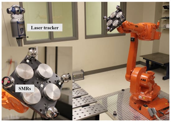
Figure 14.
Layout of four SMRs for 6D pose measuring [125].
6.2. Optical CMM
Compared to the laser tracker, optical CMM uses cameras to locate the 3D position of the target referring to the camera coordinate system. There are two types of optical CMMs regarding the target mechanism.
- A black and white ring is used as the target for position recognition, which is shown as markers in Figure 15. These markers are normally adopted by 3D camera systems. In addition to the stereo cameras, illuminations are provided to offer appropriate light for marker recognition. According to the measurement volume, the measurement accuracy is up to 6 µm [45].
- An infrared light-emitting diode (LED) is used as the target. As shown in Figure 16, three infrared line scan cameras are used to estimate the 3D position of the LEDs. The product specification of the Nikon Metrology K610 (Nikon, Tokyo, Japan) states a volumetric precision of 60 µm, depending on the measurement situation (distance and inclination towards the camera, ambient light conditions) [44].

Figure 15.
3D camera measurement system [45].

Figure 16.
All system components of the Nikon Metrology K610 [44].
Both types of targets can be very convenient to stick to the measuring object. In particular, black and white rings are very suitable for measuring a large number of components. When the 3D/6D deformation of each arm needs to be measured, at least three targets are attached to the arms (Figure 17).
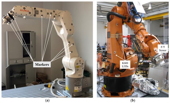
Figure 17.
3D/6D deformation measurement: (a) black and white rings are stuck on the arms and (b) LEDs are stuck on the arms [117].
Both measuring techniques have their advantages and disadvantages. The laser tracker has a larger measuring range and is not affected by ambient light. Due to the size and price of the SMR, a laser tracker is normally used to measure the displacement of the robot EE. Optical CMM is adopted to measure not only the displacement of the robot EE but also the deformation between the arms (joint deformation). When the stiffness modelling is built with the VJM method, the joint stiffness needs to be identified. Direct joint deformation measurement provides more precise information for joint stiffness identification. When only robot EE deformation is provided, the joint deformation is estimated by decoupling the robot EE deformation to each joint based on the inverse kinematics of the robot. However, the ambient light and the measuring volume should be considered if the optical CMM is appropriate for the size of the robot. In addition, the targets should be confirmed to be recognized when the robot moves to different positions.
7. Conclusions and Outlook
In various machining processes, the low stiffness of industrial robots inevitably leads to processing deformation. This problem is not prominent in ordinary handling, welding, laser cutting, etc. However, continuously high processing forces occur during machining, such as milling, drilling, and incremental sheet forming. The low stiffness of a robot causes the robot joints, mechanical arms, transmission structure, and other structures to deform, which greatly reduces the positioning accuracy of the robot; thus, it is difficult to use robots in high-precision machining [103,108,115]. To overcome this problem, deformation compensation based on a stiffness model is used to improve the machining accuracy of industrial robots. Different stiffness modelling methods were discussed and summarized in this paper.
Robot deformation compensation based on a stiffness model encounters the following issues:
- Simplifying the stiffness identification process while maintaining accuracy.
- In the process of robot processing, there are possible delays from measured wrenches due to the calculated error deformation and the feedback position compensation of the system.
- Position deviations are caused by external wrench impacts when a robot enters and exits the machining process. The dynamic characteristics of the stiffness compensation should be considered.
There are multiple challenging problems in modelling the stiffness of industrial robots. To improve stiffness models, further research can be conducted in the following areas:
- Standardization of stiffness modelling. At present, there is no standard procedure for establishing a stiffness model. It is difficult to select and apply one type of modelling method conveniently and quickly. With in-depth research on stiffness modelling methods, a modelling process with standard modelling principles, evaluation indicators, and measuring techniques could be developed.
- Automating measuring and modelling. In terms of actual measurements and stiffness modelling, the workload of manual participation can be reduced, and a set of automated systems for measuring and modelling various scenarios can be developed.
- Application of machine learning (ML) methods for stiffness modelling [43,126,127]. A high-precision stiffness model can be obtained after processing the experimental data with various artificial neural networks (ANNs). A self-learning process for stiffness modelling can also be developed and automated based on ML.
Funding
This work was supported by the State Key Laboratory of Digital Manufacturing Equipment and Technology, Grant No. DMETKF2021018.
Conflicts of Interest
The authors declare no conflict of interest.
References
- Kainrath, M.; Aburaia, M.; Stuja, K.; Lackner, M.; Markl, E. Accuracy Improvement and Process Flow Adaption for Robot Machining; Springer International Publishing: Cham, Switzerland, 2020; ISBN 9783030627836. [Google Scholar]
- Zhu, D.; Feng, X.; Xu, X.; Yang, Z.; Li, W.; Yan, S.; Ding, H. Robotic grinding of complex components: A step towards efficient and intelligent machining–challenges, solutions, and applications. Robot. Comput. Manuf. 2020, 65, 101908. [Google Scholar] [CrossRef]
- IFR. IFR Presents World Robotics Report. 2020. Available online: https://ifr.org/ifr-press-releases/news/record-2.7-million-robots-work-in-factories-around-the-globe (accessed on 17 September 2021).
- Tao, B.; Zhao, X.; Ding, H. Mobile-robotic machining for large complex components: A review study. Sci. China Technol. Sci. 2019, 62, 1388–1400. [Google Scholar] [CrossRef]
- Iglesias, I.; Sebastián, M.; Ares, J. Overview of the State of Robotic Machining: Current Situation and Future Potential. Procedia Eng. 2015, 132, 911–917. [Google Scholar] [CrossRef]
- Ji, W.; Wang, L. Industrial robotic machining: A review. Int. J. Adv. Manuf. Technol. 2019, 103, 1239–1255. [Google Scholar] [CrossRef]
- Karim, A.; Verl, A. Challenges and Obstacles in Robot-Machining. In Proceedings of the IEEE ISR 2013, Seoul, Korea, 24–26 October 2013; pp. 1–4. [Google Scholar]
- Möller, C.; Schmidt, H.C.; Koch, P.; Böhlmann, C.; Kothe, S.; Wollnack, J.; Hintze, W. Machining of large scaled CFRP-Parts with mobile CNC-based robotic system in aerospace industry. Procedia Manuf. 2017, 14, 17–29. [Google Scholar] [CrossRef]
- DeVlieg, R. High-Accuracy Robotic Drilling/Milling of 737 Inboard Flaps. SAE Int. J. Aerosp. 2011, 4, 1373–1379. [Google Scholar] [CrossRef]
- Cheng, K. (Ed.) Machining Dynamics: Theory, Applications and Practices; Springer: London, UK, 2009; ISBN 978-1-84628-368-0. [Google Scholar]
- Pandremenos, J.; Doukas, C.; Stavropoulos, P.; Chryssolouris, G. Machining With Robots: A Critical Review. In Proceedings of the 7th International Conference on Digital Enterprise Technology, Athens, Greece, 28–30 September 2011; pp. 1–9. [Google Scholar]
- Chen, Y.; Dong, F. Robot machining: Recent development and future research issues. Int. J. Adv. Manuf. Technol. 2012, 66, 1489–1497. [Google Scholar] [CrossRef]
- Khalil, W.; Dombre, E. Introduction to geometric and kinematic modeling of parallel robots. In Modeling, Identification and Control of Robots; Elsevier: Amsterdam, The Netherlands, 2002; pp. 171–190. [Google Scholar] [CrossRef]
- Pan, Z.; Zhang, H.; Zhu, Z.; Wang, J. Chatter analysis of robotic machining process. J. Mater. Process. Technol. 2006, 173, 301–309. [Google Scholar] [CrossRef]
- Yuan, L.; Pan, Z.; Ding, D.; Sun, S.; Li, W. A Review on Chatter in Robotic Machining Process Regarding Both Regenerative and Mode Coupling Mechanism. IEEE/ASME Trans. Mechatron. 2018, 23, 2240–2251. [Google Scholar] [CrossRef]
- Alici, G.; Shirinzadeh, B. Enhanced stiffness modeling, identification and characterization for robot manipulators. IEEE Trans. Robot. 2005, 21, 554–564. [Google Scholar] [CrossRef]
- Xiong, G.; Ding, Y.; Zhu, L. Stiffness-based pose optimization of an industrial robot for five-axis milling. Robot. Comput. Manuf. 2018, 55, 19–28. [Google Scholar] [CrossRef]
- Sun, L.; Liang, F.; Fang, L. Chatter Vibration Analysis of A Novel Industrial Robot for Robotic Boring Process. In Proceedings of the IEEE International Conference on Intelligence and Safety for Robotics (ISR), Shenyang, China, 24–27 August 2018; pp. 56–60. [Google Scholar] [CrossRef]
- Celikag, H.; Sims, N.D.; Ozturk, E. Cartesian Stiffness Optimization for Serial Arm Robots. Procedia CIRP 2018, 77, 566–569. [Google Scholar] [CrossRef]
- Chen, S.; Zhang, T.; Shao, M. A 6-DOF articulated robot stiffness research. In Proceedings of the 12th World Congress on Intelligent Control and Automation (WCICA), Guilin, China, 12–15 June 2016; pp. 3230–3235. [Google Scholar] [CrossRef]
- Gonçalves, R.S.; Carvalho, J.C.M. Stiffness Analysis of Parallel Manipulator Using Matrix Structural Analysis. In Proceedings of the EUCOMES 08, Cassino, Italy, 17–20 September 2008; pp. 255–262. [Google Scholar] [CrossRef]
- Olabi, A.; Damak, M.; Bearee, R.; Gibaru, O.; Leleu, S. Improving the accuracy of industrial robots by offline compensation of joints errors. In Proceedings of the IEEE International Conference on Industrial Technology, Athens, Greece, 19–21 March 2012; pp. 492–497. [Google Scholar] [CrossRef]
- Roth, Z.; Mooring, B.; Ravani, B. An overview of robot calibration. IEEE J. Robot. Autom. 1987, 3, 377–385. [Google Scholar] [CrossRef]
- Jang, J.H.; Kim, S.H.; Kwak, Y.K. Calibration of geometric and non-geometric errors of an industrial robot. Robotica 2001, 19, 311–321. [Google Scholar] [CrossRef]
- Lehmann, C.; Halbauer, M.; Euhus, D.; Overbeck, D. Milling with Industrial Robots: Strategies to Reduce and Compensate Process Force Induced Accuracy Influences. In Proceedings of the 2012 IEEE 17th International Conference on Emerging Technologies & Factory Automation (ETFA 2012), Krakow, Poland, 17–21 September 2012; pp. 1–4. [Google Scholar]
- Pan, Z.; Zhang, H. Robotic machining from programming to process control: A complete solution by force control. Ind. Robot. Int. J. Robot. Res. Appl. 2008, 35, 400–409. [Google Scholar] [CrossRef]
- Klimchik, A.; Pashkevich, A. Serial vs. quasi-serial manipulators: Comparison analysis of elasto-static behaviors. Mech. Mach. Theory 2017, 107, 46–70. [Google Scholar] [CrossRef]
- Gong, C.; Yuan, J.; Ni, J. Nongeometric error identification and compensation for robotic system by inverse calibration. Int. J. Mach. Tools Manuf. 2000, 40, 2119–2137. [Google Scholar] [CrossRef]
- Xu, P.; Yao, X.; Liu, S.; Wang, H.; Liu, K.; Kumar, A.S.; Lu, W.F.; Bi, G. Stiffness modeling of an industrial robot with a gravity compensator considering link weights. Mech. Mach. Theory 2021, 161, 104331. [Google Scholar] [CrossRef]
- Klimchik, A.; Wu, Y.; Dumas, C.; Caro, S.; Furet, B.; Pashkevich, A. Identification of geometrical and elastostatic parameters of heavy industrial robots. In Proceedings of the IEEE International Conference on Robotics and Automation, Karlsruhe, Germany, 6–10 May 2013; pp. 3707–3714. [Google Scholar] [CrossRef]
- Shchurova, E.I. Industrial Manipulating Robot Finite Element Mesh Generation Based on Robot Voxel Model; Springer International Publishing: Cham, Switzerland, 2021; ISBN 9783030548179. [Google Scholar]
- Klimchik, A.; Ambiehl, A.; Garnier, S.; Furet, B.; Pashkevich, A. Comparison Study of Industrial Robots for High-Speed Machining. In Lecture Notes in Mechanical Engineering; Springer: Cham, Switzerland, 2016; pp. 135–149. [Google Scholar] [CrossRef]
- Verl, A.; Valente, A.; Melkote, S.; Brecher, C.; Ozturk, E.; Tunc, L.T. Robots in machining. CIRP Ann. 2019, 68, 799–822. [Google Scholar] [CrossRef]
- Sun, L.; Liang, F.; Fang, L. Comparative Study of Stiffness Modeling Methods for A Novel Industrial Robotic Arm with Hybrid Open-and Closed-Loop Kinematic Chains. In Proceedings of the 2018 IEEE International Conference on Mechatronics and Automation (ICMA), Changchun, China, 5–8 August 2018; pp. 1765–1770. [Google Scholar] [CrossRef]
- Olsson, T.; Haage, M.; Kihlman, H.; Johansson, R.; Nilsson, K.; Robertsson, A.; Björkman, M.; Isaksson, R.; Ossbahr, G.; Brogårdh, T. Cost-efficient drilling using industrial robots with high-bandwidth force feedback. Robot. Comput. Manuf. 2009, 26, 24–38. [Google Scholar] [CrossRef]
- Guo, Y.; Dong, H.; Wang, G.; Ke, Y. Vibration analysis and suppression in robotic boring process. Int. J. Mach. Tools Manuf. 2016, 101, 102–110. [Google Scholar] [CrossRef]
- ABB IRB6660 Industrial Robot. Available online: https://new.abb.com/products/robotics/industrial-robots/irb-6660 (accessed on 28 January 2022).
- KUKA KR 500 FORTEC. Available online: https://www.kuka.com/en-us/products/robotics-systems/industrial-robots/kr-500-fortec (accessed on 28 January 2022).
- Kim, Y.G.; Jeong, K.S.; Gil Lee, D.; Lee, J.W. Development of the composite third robot arm of the six-axis articulated robot manipulator. Compos. Struct. 1996, 35, 331–342. [Google Scholar] [CrossRef]
- Honarpardaz, M.; Trangard, A.; Derkx, J.; Feng, X.; Shoykhet, B. Benchmark of advanced structural materials for lightweight design of industrial robots. In Proceedings of the IEEE International Conference on Industrial Technology (ICIT), Seville, Spain, 17–19 March 2015; pp. 3178–3183. [Google Scholar] [CrossRef]
- Ligang, Y.; Li, J.; Liu, X.; Dong, H. The Multi-Section Design of a Novel Soft Pneumatic Robot Arm with Variable Stiffness; Springer International Publishing: Cham, Switzerland, 2019; Volume 11740, ISBN 9783030275259. [Google Scholar]
- Klimchik, A.; Ambiehl, A.; Garnier, S.; Furet, B.; Pashkevich, A. Efficiency evaluation of robots in machining applications using industrial performance measure. Robot. Comput. Manuf. 2017, 48, 12–29. [Google Scholar] [CrossRef]
- Nguyen, V.; Cvitanic, T.; Melkote, S. Data-Driven Modeling of the Modal Properties of a Six-Degrees-of-Freedom Industrial Robot and Its Application to Robotic Milling. J. Manuf. Sci. Eng. 2019, 141, 1–24. [Google Scholar] [CrossRef]
- Johnen, B.; Scheele, C.; Kuhlenkotter, B. Learning robot behavior with artificial neural networks and a coordinate measuring machine. In Proceedings of the 5th International Conference on Automation, Robotics and Applications, Wellington, New Zealand, 6–8 December 2011; pp. 208–213. [Google Scholar] [CrossRef]
- Wu, K.; Brueninghaus, J.; Johnen, B.; Kuhlenkoetter, B. Applicability of stereo high speed camera systems for robot dynamics analysis. In Proceedings of the International Conference on Control, Automation and Robotics, Singapore, 20–22 May 2015; pp. 44–48. [Google Scholar] [CrossRef]
- Radiology, E.; Society, A. Position Control of an Industrial Robot Using an Optical Measurement System for Machining Purposes. In Proceedings of the 11th International Conference on Manufacturing Research (ICMR2013), Cranfield, UK, 19–20 September 2013; pp. 177–186. [Google Scholar]
- Shi, X.; Zhang, F.; Qu, X.; Liu, B. An online real-time path compensation system for industrial robots based on laser tracker. Int. J. Adv. Robot. Syst. 2016, 13. [Google Scholar] [CrossRef]
- Kubela, T.; Pochyly, A.; Singule, V. High Accurate Robotic Machining Based on Absolute Part Measuring and On-Line Path Compensation. In Proceedings of the 2019 International Conference on Electrical Drives & Power Electronics (EDPE), The High Tatras, Slovakia, 24–26 September 2019; pp. 143–148. [Google Scholar]
- Frommknecht, A.; Kuehnle, J.; Effenberger, I.; Pidan, S. Multi-sensor measurement system for robotic drilling. Robot. Comput. Manuf. 2017, 47, 4–10. [Google Scholar] [CrossRef]
- Shu, T.; Gharaaty, S.; Xie, W.; Joubair, A.; Bonev, I.A. Dynamic Path Tracking of Industrial Robots With High Accuracy Using Photogrammetry Sensor. IEEE/ASME Trans. Mechatron. 2018, 23, 1159–1170. [Google Scholar] [CrossRef]
- Buondonno, G.; De Luca, A. Efficient Computation of Inverse Dynamics and Feedback Linearization for VSA-Based Robots. IEEE Robot. Autom. Lett. 2016, 1, 908–915. [Google Scholar] [CrossRef]
- Belfiore, N.P.; Verotti, M.; Di Giamberardino, P.; Rudas, I.J. Active Joint Stiffness Regulation to Achieve Isotropic Compliance in the Euclidean Space. J. Mech. Robot. 2012, 4, 041010. [Google Scholar] [CrossRef]
- Flacco, F.; De Luca, A.; Sardellitti, I.; Tsagarakis, N.G. On-line estimation of variable stiffness in flexible robot joints. Int. J. Robot. Res. 2012, 31, 1556–1577. [Google Scholar] [CrossRef]
- Cordes, M.; Hintze, W. Offline simulation of path deviation due to joint compliance and hysteresis for robot machining. Int. J. Adv. Manuf. Technol. 2016, 90, 1075–1083. [Google Scholar] [CrossRef]
- Klimchik, A.; Pashkevich, A.; Chablat, D.; Hovland, G. Compliance error compensation technique for parallel robots composed of non-perfect serial chains. Robot. Comput. Manuf. 2012, 29, 385–393. [Google Scholar] [CrossRef]
- Boby, R.A.; Klimchik, A. Combination of geometric and parametric approaches for kinematic identification of an industrial robot. Robot. Comput. Manuf. 2021, 71, 102142. [Google Scholar] [CrossRef]
- Zaeh, M.F.; Roesch, O. Improvement of the machining accuracy of milling robots. Prod. Eng. 2014, 8, 737–744. [Google Scholar] [CrossRef]
- Jaca, N.A.; Amilibia, J.L.; Garmendia, I.U.; Hidalgo, I.I. Industrial Robotics Trajectory Compensation Model and Joints Torsional Stiffness Impact Analysis. In Proceedings of the 6th International Conference on Control, Automation and Robotics (ICCAR), Singapore, 20–23 April 2020; pp. 101–106. [Google Scholar] [CrossRef]
- Klimchik, A.; Pashkevich, A.; Chablat, D. CAD-based approach for identification of elasto-static parameters of robotic manipulators. Finite Elements Anal. Des. 2013, 75, 19–30. [Google Scholar] [CrossRef]
- Kim, S.H.; Nam, E.; Ha, T.I.; Hwang, S.-H.; Lee, J.H.; Park, S.-H.; Min, B.-K. Robotic Machining: A Review of Recent Progress. Int. J. Precis. Eng. Manuf. 2019, 20, 1629–1642. [Google Scholar] [CrossRef]
- Gonçalves, R.; Carbone, G.; Carvalho, J.; Ceccarelli, M. A Comparison of Stiffness Analysis Methods for Robotic Systems. Int. J. Mech. Control 2016, 17, 35–58. [Google Scholar]
- Kefer, M.; Zhang, J.; Xie, H. A versatile, non-linear and elasto-static stiffness model of articulated industrial robots. In Proceedings of the IEEE International Conference on Automation Science and Engineering (CASE), New Taipei, Taiwan, 18–22 August 2014; pp. 208–214. [Google Scholar] [CrossRef]
- Klimchik, A.; Pashkevich, A.; Chablat, D. Fundamentals of manipulator stiffness modeling using matrix structural analysis. Mech. Mach. Theory 2019, 133, 365–394. [Google Scholar] [CrossRef]
- Mousavi, S.; Gagnol, V.; Bouzgarrou, B.C.; Ray, P. Model-Based Stability Prediction of a Machining Robot. In Mechanisms and Machine Science; Springer: Cham, Switzerland, 2016; pp. 379–387. [Google Scholar] [CrossRef]
- Detert, T.; Corves, B. Extended Procedure for Stiffness Modeling Based on the Matrix Structure Analysis. In Mechanisms and Machine Science; Springer: Cham, Switzerland, 2016; pp. 299–310. [Google Scholar] [CrossRef]
- Klimchik, A.; Furet, B.; Caro, S.; Pashkevich, A. Identification of the manipulator stiffness model parameters in industrial environment. Mech. Mach. Theory 2015, 90, 1–22. [Google Scholar] [CrossRef]
- Avilés, R.; Ajuria, M.G.; Hormaza, M.V.; Hernández, A. A procedure based on finite elements for the solution of nonlinear problems in the kinematic analysis of mechanisms. Finite Elements Anal. Des. 1996, 22, 305–327. [Google Scholar] [CrossRef]
- Salisbury, J. Active Stiffness Control of a Manipulator in Cartesian Coordinates. In Proceedings of the 19th IEEE Conference on Decision and Control including the Symposium on Adaptive Processes, Albuquerque, NM, USA, 10–12 December 1980; pp. 95–100. [Google Scholar]
- Cheng, S.-F.; Kao, I. Simulation of conservative properties of stiffness matrices in congruence transformation. In Proceedings of IEEE/RSJ International Conference on Intelligent Robots and Systems. Innovations in Theory, Practice and Applications (Cat. No.98CH36190), Victoria, BC, Canada, 13–17 October 1998; Volume 1, pp. 311–316. [Google Scholar] [CrossRef]
- Kao, I.; Ngo, C. Properties of Grasp Stiffness Matrix and Conservative Control Strategy. Int. J. Robot. Res. 1999, 18, 159–167. [Google Scholar] [CrossRef]
- Siciliano, B. Kinematic control of redundant robot manipulators: A tutorial. J. Intell. Robot. Syst. 1990, 3, 201–212. [Google Scholar] [CrossRef]
- Dumas, C.; Caro, S.; Garnier, S.; Furet, B. Joint stiffness identification of six-revolute industrial serial robots. Robot. Comput. Manuf. 2011, 27, 881–888. [Google Scholar] [CrossRef]
- Angeles, J. On the Nature of the Cartesian Stiffness Matrix. Ing. Mecánica Tecnol. Desarro 2010, 3, 163–170. [Google Scholar]
- Ajoudani, A.; Tsagarakis, N.G.; Bicchi, A. On the role of robot configuration in Cartesian stiffness control. In Proceedings of the IEEE International Conference on Robotics and Automation (ICRA), Seattle, WA, USA, 26–30 May 2015; pp. 1010–1016. [Google Scholar] [CrossRef]
- Chen, C.; Peng, F.; Yan, R.; Li, Y.; Wei, D.; Fan, Z.; Tang, X.; Zhu, Z. Stiffness performance index based posture and feed orientation optimization in robotic milling process. Robot. Comput. Manuf. 2018, 55, 29–40. [Google Scholar] [CrossRef]
- Verotti, M.; Masarati, P.; Morandini, M.; Belfiore, N. Isotropic compliance in the Special Euclidean Group SE(3). Mech. Mach. Theory 2016, 98, 263–281. [Google Scholar] [CrossRef]
- Carbone, G.; Ceccarelli, M. Comparison of indices for stiffness performance evaluation. Front. Mech. Eng. China 2010, 5, 270–278. [Google Scholar] [CrossRef]
- Sabourin, L.; Subrin, K.; Cousturier, R.; Gogu, G.; Mezouar, Y. Redundancy-based optimization approach to optimize robotic cell behaviour: Application to robotic machining. Ind. Robot. Int. J. Robot. Res. Appl. 2015, 42, 167–178. [Google Scholar] [CrossRef]
- Lin, J.; Ye, C.; Yang, J.; Zhao, H.; Ding, H.; Luo, M. Contour error-based optimization of the end-effector pose of a 6 degree-of-freedom serial robot in milling operation. Robot. Comput. Manuf. 2021, 73, 102257. [Google Scholar] [CrossRef]
- Bayo, E. A finite-element approach to control the end-point motion of a single-link flexible robot. J. Robot. Syst. 1987, 4, 63–75. [Google Scholar] [CrossRef]
- Corradini, C.; Fauroux, J.; Krut, S.; Company, O. Evaluation of a 4-Degree of Freedom Parallel Manipulator Stiffness. In Proceedings of the 11th World Congress in Mechanism and Machine Science, Tianjin, China, 18–21 August 2003. [Google Scholar]
- Bouzgarrou, B.C.; Fauroux, J.C.; Gogu, G.; Heerah, Y. Rigidity Analysis of T3R1 Parallel Robot with Uncoupled Kinematics. In Proceedings of the 35th International Symposium on Robotics, Paris, France, 23–26 March 2004. [Google Scholar]
- Pashkevich, A.; Chablat, D.; Wenger, P. Stiffness analysis of overconstrained parallel manipulators. Mech. Mach. Theory 2009, 44, 966–982. [Google Scholar] [CrossRef]
- Cao, W.-A.; Ding, H. A method for stiffness modeling of 3R2T overconstrained parallel robotic mechanisms based on screw theory and strain energy. Precis. Eng. 2018, 51, 10–29. [Google Scholar] [CrossRef]
- Rizk, R.; Fauroux, J.-C.; Munteanu, M.G.; Gogu, G. A Comparative Stiffness Analysis of a Reconfigurable Parallel Machine with Three or Four Degrees of Mobility. J. Mach. Eng. 2006, 6, 45–55. [Google Scholar]
- Yang, C.; Li, Q.; Chen, Q.; Xu, L. Elastostatic stiffness modeling of overconstrained parallel manipulators. Mech. Mach. Theory 2018, 122, 58–74. [Google Scholar] [CrossRef]
- Shi, S.; Wu, H.; Song, Y.; Handroos, H.; Li, M.; Cheng, Y.; Mao, B. Static stiffness modelling of EAST articulated maintenance arm using matrix structural analysis method. Fusion Eng. Des. 2017, 124, 507–511. [Google Scholar] [CrossRef]
- Liu, H.; Huang, T.; Chetwynd, D.G.; Kecskemethy, A. Stiffness Modeling of Parallel Mechanisms at Limb and Joint/Link Levels. IEEE Trans. Robot. 2017, 33, 734–741. [Google Scholar] [CrossRef]
- Zhao, C.; Guo, H.; Zhang, D.; Liu, R.; Li, B.; Deng, Z. Stiffness modeling of n(3RRlS) reconfigurable series-parallel manipulators by combining virtual joint method and matrix structural analysis. Mech. Mach. Theory 2020, 152, 103960. [Google Scholar] [CrossRef]
- Klimchik, A.; Pashkevich, A.; Caro, S.; Chablat, D. Stiffness Matrix of Manipulators With Passive Joints: Computational Aspects. IEEE Trans. Robot. 2012, 28, 955–958. [Google Scholar] [CrossRef]
- Azulay, H.; Mahmoodi, M.; Zhao, R.; Mills, J.K.; Benhabib, B. Comparative analysis of a new 3×PPRS parallel kinematic mechanism. Robot. Comput. Manuf. 2014, 30, 369–378. [Google Scholar] [CrossRef]
- Ghali, A.; Neville, A. Structural Analysis, a Unified Classical and Matrix Approach; Taylor and Francis: Abingdon-on-Thames, UK, 2017; Volume 2, ISBN 9781315266930. [Google Scholar]
- Clinton, C.; Zhang, G.; Wavering, A.J. Stiffness Modeling of a Stewart-Platform-Based Milling Machine; DRUM: College Park, MD, USA, 1997. [Google Scholar] [CrossRef]
- Lu, Y.; Dai, Z.; Ye, N. Stiffness analysis of parallel manipulators with linear limbs by considering inertial wrench of moving links and constrained wrench. Robot. Comput. Manuf. 2017, 46, 58–67. [Google Scholar] [CrossRef]
- Subrin, K.; Sabourin, L.; Cousturier, R.; Gogu, G.; Mezouar, Y. New Redundant Architectures in Machining: Serial and Parallel Robots. Procedia Eng. 2013, 63, 158–166. [Google Scholar] [CrossRef][Green Version]
- Wang, Y.; Zhang, R.; Ju, F.; Zhao, J.; Chen, B.; Wu, H. A light cable-driven manipulator developed for aerial robots: Structure design and control research. Int. J. Adv. Robot. Syst. 2020, 17. [Google Scholar] [CrossRef]
- Asada, H.; Youcef-Toumi, K.; Lim, S.K. Joint Torque Measurement of a Direct-Drive Arm. In Proceedings of the 23rd IEEE Conference on Decision and Control, Las Vegas, NV, USA, 14 December 1984; pp. 1332–1337. [Google Scholar]
- Yang, K.; Yang, W.; Cheng, G.; Lu, B. A new methodology for joint stiffness identification of heavy duty industrial robots with the counterbalancing system. Robot. Comput. Manuf. 2018, 53, 58–71. [Google Scholar] [CrossRef]
- Hui, Z.; Jianjun, W.; Zhang, G.; Zhongxue, G.; Zengxi, P.; Hongliang, C.; Zhenqi, Z. Machining with Flexible Manipulator: Toward Improving Robotic Machining Performance. In Proceedings of the 2005 IEEE/ASME International Conference on Advanced Intelligent Mechatronics, Monterey, CA, USA, 24–28 July 2005; pp. 1127–1132. [Google Scholar]
- Pan, Z.; Zhang, H. Improving Robotic Machining Accuracy by Real-Time Compensation. In Proceedings of the 2009 ICCAS-SICE, Fukuoka, Japan, 18–21 August 2009; pp. 4289–4294. [Google Scholar]
- Abele, E.; Rothenbücher, S.; Weigold, M. Cartesian compliance model for industrial robots using virtual joints. Prod. Eng. 2008, 2, 339–343. [Google Scholar] [CrossRef]
- Abele, E.; Weigold, M.; Rothenbücher, S. Modeling and Identification of an Industrial Robot for Machining Applications. CIRP Ann. 2007, 56, 387–390. [Google Scholar] [CrossRef]
- Slavkovic, N.R.; Milutinovic, D.; Glavonjic, M.M. A method for off-line compensation of cutting force-induced errors in robotic machining by tool path modification. Int. J. Adv. Manuf. Technol. 2013, 70, 2083–2096. [Google Scholar] [CrossRef]
- Tsumugiwa, T.; Fukui, Y.; Yokogawa, R. Compliance measurement for the Mitsubishi PA-10 robot. Adv. Robot. 2014, 28, 919–928. [Google Scholar] [CrossRef]
- Chen, S.-F.; Kao, I. Conservative Congruence Transformation for Joint and Cartesian Stiffness Matrices of Robotic Hands and Fingers. Int. J. Robot. Res. 2000, 19, 835–847. [Google Scholar] [CrossRef]
- Chen, S. The 6x6 Stiffness Formulation and Transformation of Serial Manipulators via the CCT Theory. In Proceedings of the IEEE International Conference on Robotics and Automation, Taipei, Taiwan, 14–19 September 2003; pp. 4042–4047. [Google Scholar]
- Alici, G.; Shirinzadeh, B. A systematic technique to estimate positioning errors for robot accuracy improvement using laser interferometry based sensing. Mech. Mach. Theory 2005, 40, 879–906. [Google Scholar] [CrossRef]
- Tyapin, I.; Kaldestad, K.B.; Hovland, G. Off-line path correction of robotic face milling using static tool force and robot stiffness. In Proceedings of the IEEE/RSJ International Conference on Intelligent Robots and Systems (IROS), Hamburg, Germany, 28 September–2 October 2015; pp. 5506–5511. [Google Scholar] [CrossRef]
- Dumas, C.; Caro, S.; Cherif, M.; Garnier, S.; Furet, B. Joint stiffness identification of industrial serial robots. Robotica 2011, 30, 649–659. [Google Scholar] [CrossRef]
- Ambiehl, A.; Garnier, S.; Subrin, K.; Furet, B. New method for decoupling the articular stiffness identification: Application to an industrial robot with double encoding system on its 3 first axis. In Proceedings of the IEEE/RSJ International Conference on Intelligent Robots and Systems (IROS), Vancouver, BC, Canada, 24–28 September 2017; pp. 1478–1483. [Google Scholar] [CrossRef]
- Guo, Y.; Dong, H.; Ke, Y. Stiffness-oriented posture optimization in robotic machining applications. Robot. Comput. Manuf. 2015, 35, 69–76. [Google Scholar] [CrossRef]
- Bu, Y.; Liao, W.; Tian, W.; Zhang, J.; Zhang, L. Stiffness analysis and optimization in robotic drilling application. Precis. Eng. 2017, 49, 388–400. [Google Scholar] [CrossRef]
- Liao, Z.-Y.; Li, J.-R.; Xie, H.-L.; Wang, Q.-H.; Zhou, X.-F. Region-based toolpath generation for robotic milling of freeform surfaces with stiffness optimization. Robot. Comput. Manuf. 2020, 64, 101953. [Google Scholar] [CrossRef]
- Zhu, Z.; Tang, X.; Chen, C.; Peng, F.; Yan, R.; Zhou, L.; Li, Z.; Wu, J. High precision and efficiency robotic milling of complex parts: Challenges, approaches and trends. Chin. J. Aeronaut. 2021, 35, 22–46. [Google Scholar] [CrossRef]
- Xiong, G.; Ding, Y.; Zhu, L. A Feed-Direction Stiffness Based Trajectory Optimization Method for a Milling Robot. In Lecture Notes in Mechanical Engineering; Springer: Cham, Switzerland, 2017; pp. 184–195. [Google Scholar] [CrossRef]
- Sun, J.; Zhang, W. Measured Stiffness Performance Evaluation Index of Industrial Robot in Side Milling. J. Phys. Conf. Ser. 2021, 1802, 022093. [Google Scholar] [CrossRef]
- Schneider, U.; Momeni, K.M.; Ansaloni, M.; Verl, A. Stiffness Modeling of Industrial Robots for Deformation Compensation in Machining. In Proceedings of the 2014 IEEE/RSJ International Conference on Intelligent Robots and Systems, Chicago, IL, USA, 14–18 September 2014; pp. 4464–4469. [Google Scholar]
- Posada, J.R.D.; Schneider, U.; Sridhar, A.; Verl, A. Automatic Motion Generation for Robotic Milling Optimizing Stiffness with Sample-Based Planning. Machines 2017, 5, 3. [Google Scholar] [CrossRef]
- Klimchik, A.; Bondarenko, D.; Pashkevich, A.; Briot, S.; Furet, B. Compensation of Tool Deflection in Robotic-Based Milling. In Proceedings of the 9th International Conference on Informatics in Control, Automation and Robotics, Rome, Italy, 28–31 July 2012; pp. 113–122. [Google Scholar]
- Klimchik, A.; Bondarenko, D.; Pashkevich, A.; Briot, S.; Furet, B.; Ferrier, J.-L.; Bernard, A.; Gusikhin, O.; Madani, K. Compliance Error Compensation in Robotic-Based Milling—Informatics in Control, Automation and Robotics. In Proceedings of the 9th International Conference, (ICINCO 2012), Rome, Italy, 28–31 July 2012; Springer International Publishing: Cham, Switzerland, 2014; Volume 283, pp. 197–216, ISBN 9783319034997. [Google Scholar]
- Klimchik, A.; Pashkevich, A. Robotic manipulators with double encoders: Accuracy improvement based on advanced stiffness modeling and intelligent control. IFAC-PapersOnLine 2018, 51, 740–745. [Google Scholar] [CrossRef]
- Lin, J.; Li, Y.; Xie, Y.; Hu, J.; Min, J. Joint stiffness identification of industrial serial robots using 3D digital image correlation techniques. Proc. Inst. Mech. Eng. Part C J. Mech. Eng. Sci. 2021, 236, 536–551. [Google Scholar] [CrossRef]
- Slamani, M.; Nubiola, A.; Bonev, I. Assessment of the positioning performance of an industrial robot. Ind. Robot. Int. J. Robot. Res. Appl. 2012, 39, 57–68. [Google Scholar] [CrossRef]
- Hexagon Leica T-Mac: 6DoF Tracking Device for Automated Applications. Available online: https://www.hexagonmi.com/products/laser-tracker-systems/leica-tmac (accessed on 20 June 2022).
- Nubiola, A.; Bonev, I.A. Absolute calibration of an ABB IRB 1600 robot using a laser tracker. Robot. Comput. Integr. Manuf. 2013, 29, 236–245. [Google Scholar] [CrossRef]
- Wang, R.; Li, F.; Niu, J.; Sun, Y. Prediction of pose-dependent modal properties and stability limits in robotic ball-end milling. Robot. Comput. Manuf. 2022, 75, 102307. [Google Scholar] [CrossRef]
- Wu, K.; Li, J. Prediction of the eigenfrequency of industrial robots based on the ANN model. In Proceedings of the China Automation Congress (CAC), Beijing, China, 22–24 October 2021; pp. 1595–1598. [Google Scholar] [CrossRef]
Publisher’s Note: MDPI stays neutral with regard to jurisdictional claims in published maps and institutional affiliations. |
© 2022 by the authors. Licensee MDPI, Basel, Switzerland. This article is an open access article distributed under the terms and conditions of the Creative Commons Attribution (CC BY) license (https://creativecommons.org/licenses/by/4.0/).