Real-Time Motion Detection Network Based on Single Linear Bottleneck and Pooling Compensation

Abstract

Motion (change) detection is a basic preprocessing step in video processing, which has many application scenarios. One challenge is that deep learning-based methods require high computation power to improve their accuracy. In this paper, we introduce a novel semantic segmentation and lightweight-based network for motion detection, called Real-time Motion Detection Network Based on Single Linear Bottleneck and Pooling Compensation (MDNet-LBPC). In the feature extraction stage, the most computationally expensive CNN block is replaced with our single linear bottleneck operator to reduce the computational cost. During the decoder stage, our pooling compensation mechanism can supplement the useful motion detection information. To our best knowledge, this is the first work to use the lightweight operator to solve the motion detection task. We show that the acceleration performance of the single linear bottleneck is $5\%$ higher than that of the linear bottleneck, which is more suitable for improving the efficiency of model inference. On the dataset CDNet2014, MDNet-LBPC increases the frames per second (FPS) metric by 123 compared to the suboptimal method FgSegNet_v2, ranking first in inference speed. Meanwhile, our MDNet-LBPC achieves $95.74\%$ on the accuracy metric, which is comparable to the state-of-the-art methods.

1. Introduction

We investigate efficient deep learning methods for motion segmentation scenarios, and focus on efficient segmentation models with proper accuracy. Such a task is also known as unsupervised video object segmentation (VOS). Motion (change) detection is a binary classification problem which refers to segmenting moving objects from video sequences. As a basic preprocessing step in video processing, it is widely employed in many visual applications such as people counting [1], object tracking [2], mobility monitoring [3] and video summary [4], etc. The common methods for detecting moving objects in a scene are background subtraction [5], point trajectory [6], over-segmentation [7], “Object-like” segments [8] and CNN-based [9] methods, in which moving objects are considered as foreground regions and non-moving objects are considered as background regions, The output of the moving objects detection process is a binary mask which divides the input frame pixels into sets of background and foreground pixels.

Background subtraction is widely used in many visual surveillance applications. There are many challenges in developing a robust background subtraction algorithm: illumination changes, shadows cast by foreground objects, dynamic background motion, camera motion, camouflage or subtle regions, i.e., similarity between foreground pixels and background pixels. In recent years, these challenges have been extensively studied and numerous approaches have been proposed [6,7,8,9,10,11,12,13,14,15,16,17,18,19,20]. Among them, some methods based on deep learning [9,10,11,12,13,14,15] have achieved great success. However, in order to solve the above challenges and eliminate the interference caused by irrelevant targets, deep learning-based methods need to pay a high computational cost, which makes them difficult to implement in real-time applications.

To solve the above efficiency problems in existing deep learning methods and improve the detection and segmentation efficiency of the model, we expect that we can accelerate the model by designing the compactness convolution structure.

Some recent studies [21,22,23,24] have shown that the bottleneck structure and deep separable convolution used in the lightweight network model can be used to reduce the complexity of the deep neural network and achieve a significant acceleration effect. Inspired by the recent success of semantic segmentation based motion detection method [9], we propose a Real-time Motion Detection Network Based on Single Linear Bottleneck and Pooling Compensation (MDNet-LBPC). This model classifies foreground and background pixels through the encoder decoder structure. Rich segmentation details and efficient segmentation can be obtained by the pooling compensation mechanism and single linear bottleneck structure. We successfully combine semantic segmentation techniques and the lightweight techniques of deep neural networks for efficient motion segmentation. Our main contributions are as follows:

•

We propose a novel real-time motion detection network based on single linear bottleneck operator and pooling compensation mechanism named MDNet-LBPC, which can achieve efficient motion detection with accurate segmentation results.

•

Based on the bottleneck structure and the invert linear bottleneck operator, we propose a single linear bottleneck operator, which can reduce the FLOPs, thereby improving the inference efficiency of the model.

•

We propose a pooling compensation technique based on attention mechanism and skip connections that can be used to compensate for the loss of information compression caused by pooling, thereby improving the accuracy of our motion detection model.

2. Related Works

We will provide a brief overview of the related works on motion detection, including conventional approaches and CNN-based methods from the perspective of computational efficiency. In addition, we also introduce the lightweight architecture-based methods which are relevant to this paper.

2.1. Conventional Methods

Most conventional approaches rely on building a background model for a specific video sequence. To model the background model, statistical (or parametric) methods using Gaussians are proposed [20,25,26] to label each pixel as a background or foreground pixel. In [27], an improved Gaussian mixture model compression technique is proposed to separate background images and moving objects in video. However, parametric methods are computationally inefficient. To alleviate this problem, various nonparametric methods [28,29,30] have been proposed.

In order to reduce the impact of lighting changes, shadows cast by foreground objects, dynamic background motion, camera motion, camouflage or subtle areas on the performance of background subtraction, A. Pante et al. [31] proposed the idea of background modeling based on frame difference. Furthermore, ref. [32] used Genetic programing to select different change detection methods and combined their results. Most of the current CNN-based methods are also based on background subtraction. However, these methods may cause overfitting due to the loss of redundant pixels and higher context information in patches, and require a large number of patches for training.

2.2. Cnn-Based Methods

Recently, CNN-based methods [10,11,12,13,33] have shown impressive results and can outperform classical approaches by large margins. Braham et al. [34] proposed the first CNN-based background subtraction method for specific scenes. First, a temporal median operation is performed on the video frames to generate a fixed background image; then, for each frame in the sequence, an image patch frame and background image centered on each pixel are extracted from the current frame. Babaee et al. [17] proposed a new background image generation and motion detector, which produces a more accurate background image. R. Gupta et al. [35] proposed a new computer vision algorithm to improve detection accuracy by using spatiotemporal features. Further optimization will reduce feature dimension by using principal component analysis to detect anomalies in a given video sequence.

Wang et al. [16] proposed a multi-scale cascaded convolutional neural network structure for background subtraction without the need to construct a background image. Recently, Lim et al. [10] proposed a semantic segmentation-based encoder–decoder neural network with triple CNN and transposed CNN configurations, which has achieved state-of-the-art performance. In the subsequent studies [9,11,13,33], the semantic segmentation-based strategy was used in the motion detection task and was able to achieve state-of-the-art performance. Although these semantic segmentation-based methods can achieve high accuracy, their inference efficiency is limited.

2.3. Lightweight Architecture

In recent years, deep neural network model compression and acceleration methods have been rapidly developed. Ji et al. [36]. summarized this work in 2018, including lightweight architecture to achieve model compression and acceleration.

Following the pioneering work of grouping/deep convolution and separation convolution, lightweight architecture design has achieved rapid development, including Xception [23], MobileNet [22,24], ShuffleNet [21], etc. The lightweight neural network is a lighter model, which has a performance no worse than that of the heavier model. It aims to further reduce the amount of model parameters and complexity on the basis of maintaining the accuracy of the model and make the operation speed faster, so as to realize a hardware-friendly neural network.

Commonly used lightweight neural network technologies include distillation, pruning, quantization, weight sharing, low-rank decomposition, lightweight attention module, dynamic network architecture/training mode, lighter network architecture design, NAS (neural architecture search), etc. These methods achieve a valuable compromise between the speed and accuracy of the classification task. We propose a new lightweight operator, called single linear bottleneck, and apply it to our motion detection network. This is the first work to use the lightweight operator to solve the motion detection task.

3. Methods

Motivated semantic segmentation-based methods [9,11,13,33] in motion detection tasks typically use lightweight operators [22,23,24,37], and here we propose a real-time motion detection network based on single-linear bottleneck and pooling compensation, MDNet-LBPC.

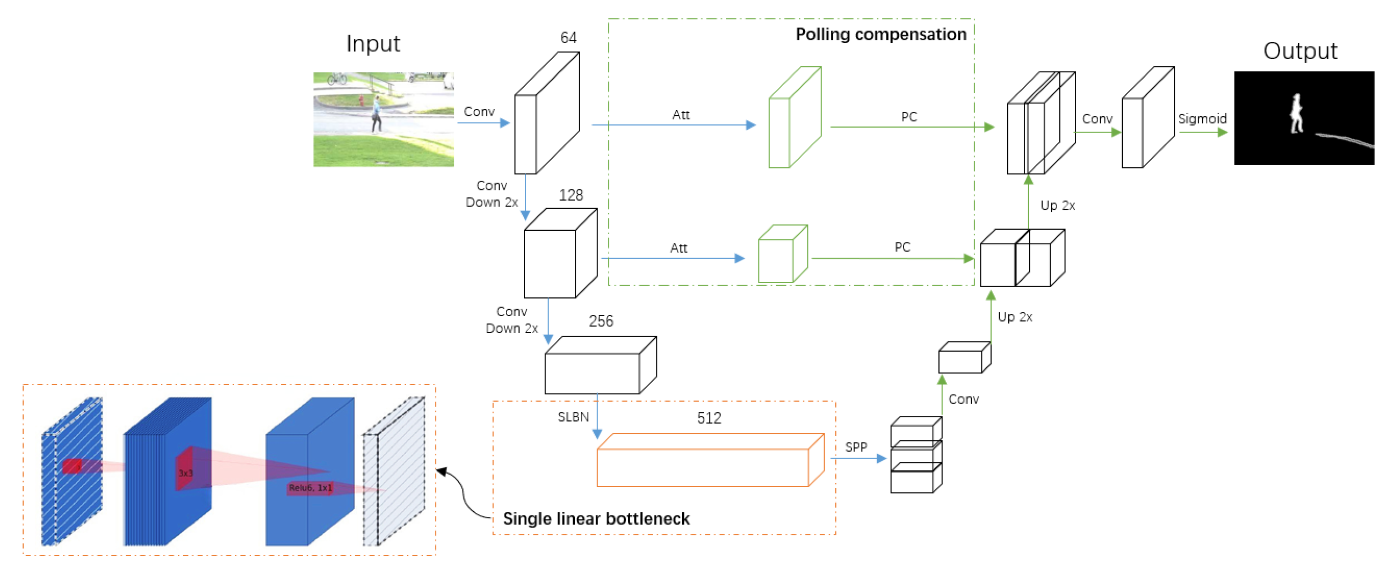
The overview of our framework is illustrated in Figure 1. In the first stage (blue), the encoder takes an RGB image as the input, and outputs multi-scale spatial feature maps. We replace the most computationally expensive CNN block with our single linear bottleneck operator to reduce the computational cost. In the second stage (green), the decoder uses the coarse probability maps and intermediate spatial feature maps from the first stage to further refine predictions through our proposed pooling compensation mechanism. At the same time, the lower left corner shows the relationship between the input and output in a single linear bottleneck operator. A single linear bottleneck block looks like a residual block, where each block contains one input, then a bottleneck, and finally an extension. However, the bottleneck actually contains all the necessary information, and the extension layer is only the implementation of the nonlinear transformation of the adjoint tensor. Therefore, we can directly use shortcuts between the bottlenecks.

We will elaborate the single linear bottleneck operator in MDNet-LBPC in Section 3.1, and the polling compensation mechanisms in MDNet-LBPC in Section 3.2. In Section 3.3, We will analyze the computational cost of our model. In Section 3.4, we will provide more implementation details.

3.1. Single Linear Bottleneck

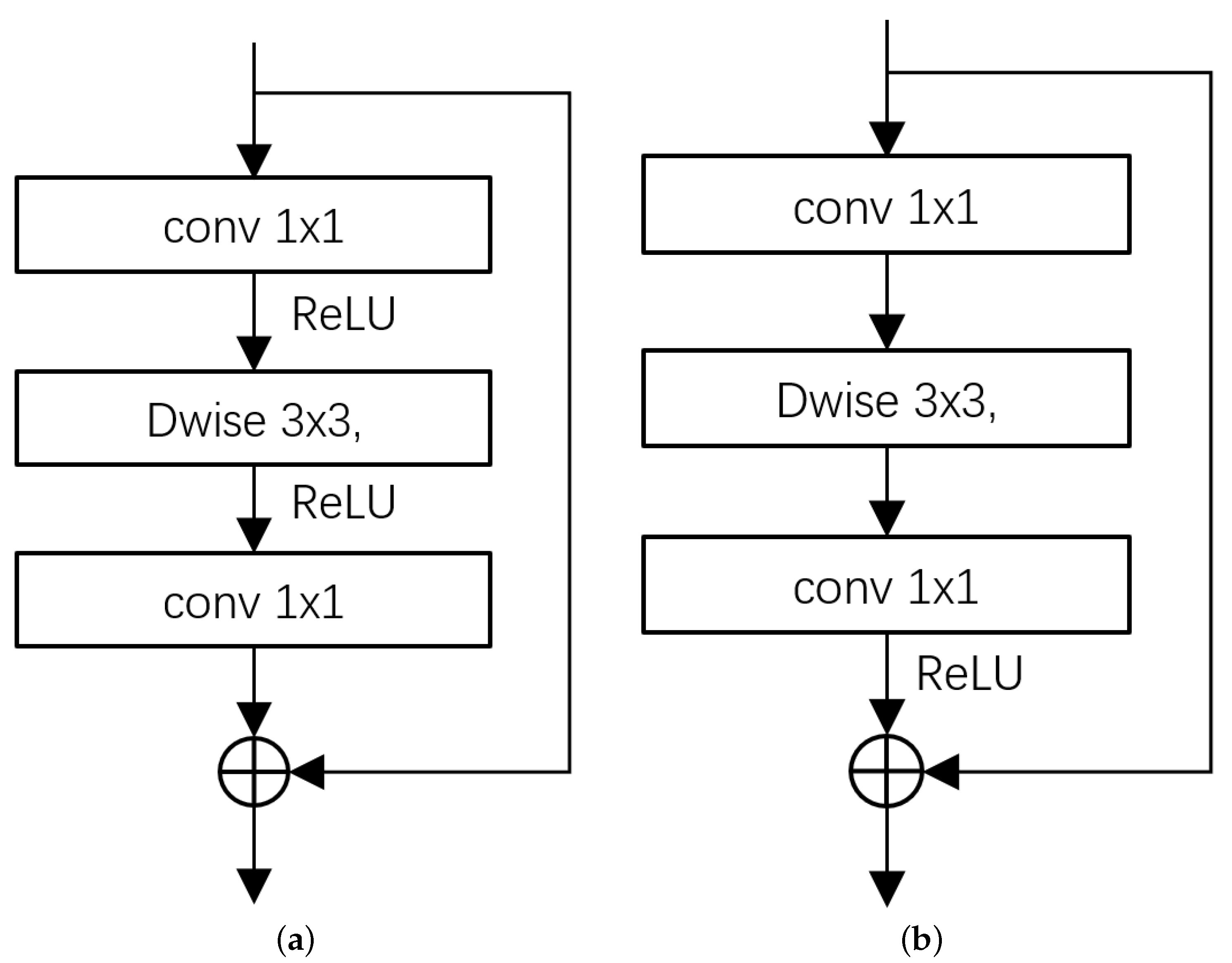
The single-linear bottleneck operator is mainly used to reduce the computational load of the model. Its structure is shown in Figure 2b. First, the channel dimension is reduced by the $1\times 1$ convolution. Then the feature map is passed through the $3\times 3$ depth-wise separable convolution. Finally the channel dimension is restored by the $1\times 1$ convolution. The nonlinear activation function ReLU is used at the bottleneck, and the other bottleneck is linear. Therefore, it is called the single-linear bottleneck structure. The design idea of the single-linear bottleneck structure will be described in details below.

He et al. [37] used the bottleneck structure to reduce the computational load of the model. However, subsequent study [24] showed that using ReLU for nonlinear activation in the bottleneck layer may lead to loss of information, especially in low-dimensional space. Considering that if the number of channels is increased in the bottleneck layer, the amount of computation will increase. Han et al. [38] used an appropriate number of ReLUs to ensure the nonlinearity of the feature space, and the remaining ReLUs can be removed to improve network performance. Shen et al. [39] set ReLU within residual units by creating identity paths. On this basis, we think that ReLU can be placed in the bottleneck structure channel recovery, which can maintain a certain nonlinearity and prevent excessive information loss. The proposed single linear bottleneck is denoted as $\mathsf{\Phi }\left(x\right)$, which can be represented by the Equation (1). $A·N$ represents the linear conversion $A:{\mathbb{R}}^{s\times s\times k}\to {\mathbb{R}}^{s_1\times s_1\times \left(tk\right)}$, B is a nonlinear transformation with $B:{\mathbb{R}}^{s_1\times s_1\times \left(tk\right)}\to {\mathbb{R}}^{s_1\times s_1\times k^{\prime }}$, where t is the channel reduction factor.

$$\mathsf{\Phi }\left(x\right)=[A·N\circ B]x$$

(1)

The detailed structure of this block is shown in

Table 1. Single linear bottleneck block transforming from k to $k^{\prime }$ channels, with stride s, and reduction factor t.

Input	Operator	Output
h × w × k	linear 1 × 1 conv2d	h × w × $\left(tk\right)$
h × w × $\left(tk\right)$	linear 3 × 3 dwise s = s	$\frac{h}{s}$ × $\frac{w}{s}$ × $\left(tk\right)$
$\frac{h}{s}$ × $\frac{w}{s}$ × $\left(tk\right)$	1 × 1 conv2d, ReLU	$\frac{h}{s}$ × $\frac{w}{s}$ × k

. During the operation, the number of channels is reduced from k to $tk$, and then expanded to $k^{\prime }$.

Formal comparison MobileNetV2 [24] is shown in Figure 2, Figure 2a is the inverted residual linear bottleneck structure. Compared with the inverted residual linear bottleneck, both bottleneck ends are linearly processed. However, the single-linear bottleneck structure only keeps one bottleneck end linear. Furthermore, compared to MobileNetV2 [24], which can only use depth-wise separable convolutions to reduce computation, our single-linear bottleneck operator simultaneously reduces computation by channel narrowing and using depth-wise separable convolutions.

3.2. Pooling Compensation

The pooling compensation mechanism proposed in this paper uses skip links to compensate for the loss of information in the encoder–decoder structure due to the compression. The main theoretical basis is the re-used feature implemented by skip links [40], on which the attention mechanism is used to enhance the desired detail regions while suppressing other irrelevant regions.

Lecun et al. [41] and Zeiler et al. [42] pointed out that pooling will bring about the loss of information, which may affect the final effect of the model. In previous studies, such as in the field of image segmentation, FCN [43] used skip links to add rich details to the segmentation results, but did not explain it theoretically. These methods did not highlight the specific needs of rich foreground target details, neither do methods such as Unet [44] and the foreground segmentation network FgSegNetV2 [9]. In other words, these methods do not achieve relevant feature enhancement and irrelevant feature suppression, while irrelevant features may have an impact on the accuracy of results. The motivation for designing the pooling compensation mechanism in this paper is based on this existing problem.

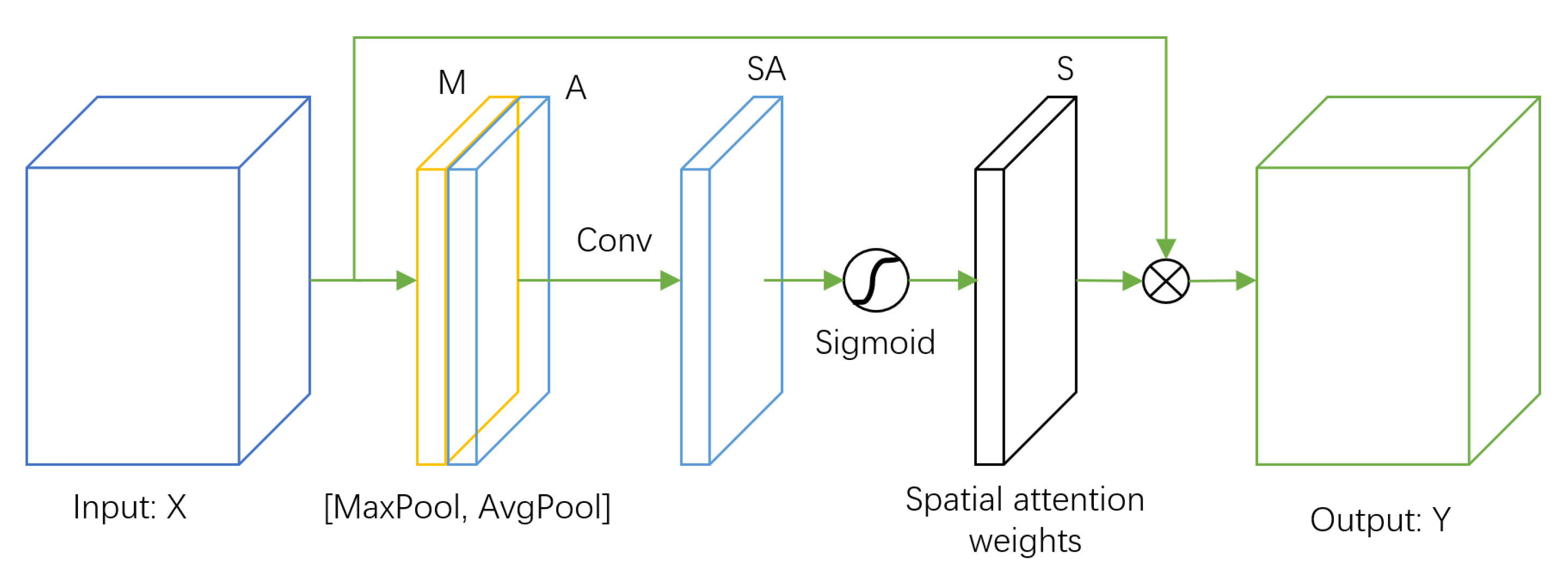
We believe that the loss of detailed information caused by pooling can be alleviated by pooling compensation. We propose the pooling compensation mechanism (Figure 3) to enhance the detailed information required for classification and suppress irrelevant information. We first perform the convolution operation of $k\times k$ on the feature map X before the maximum pooling operation to obtain the feature map $SX$. We then obtain the corresponding weight matrix S through the Sigmoid activation process, and finally input the feature. The image X and the weight matrix S are multiplied to obtain the weighted output feature map Y, as shown in Equation (2). The importance of each pixel on the input feature map for subsequent classification is obtained by the learning. Hence, we can enhance the feature details of the pooling loss and suppress the irrelevant regions.

$$Y=\sigma \left(f^{k\times k}X\right)X$$

(2)

where $\sigma$ is the sigmoid activation operation, and $f^{k\times k}$ represents the $k\times k$ convolution operation.

3.3. Computational Analysis

The lightweight of FSNet-LBPC is mainly reflected in the use of the single-linear bottleneck operator. In this section, we will first compare the computational load of similar operators, and then compare the computational load of similar models.

Comparison of different bottlenecks. We set 3 standard convolutional layers of 3 × 3 as the benchmark.

Table 2. Comparing the computation and parameters of different bottlenecks. The best scores are marked in bold.

Input Feature Map Size: $14\times 14\times 512$
Module Settings	Baseline	Bottleneck [37]	Ivert LB [24]	Our
FLOPs	$1.4\times {10}^9$	$1.9\times {10}^8$	$1.6\times {10}^8$	6.5 $\times {10}^7$
Params	$7.1\times {10}^6$	$2.6\times {10}^6$	$9.9\times {10}^5$	4.0 $\times {10}^5$

shows the comparison results: compared with similar operators, the computational complexity of the single-linear bottleneck operator is reduced by an order of magnitude.

Comparison of similar models.

Table 3. Computational comparison with state-of-the-art methods. The best scores are marked in bold.

Input Feature Map Size: $112\times 112\times 3$
Method	MDNet-LBPC	FgSegNet_v2 [9]	FgSegNet_S [15]	FgSegNet [10]	MU-Net2 [13]
FLOPs	$2.4\times {10}^9$	$7.2\times {10}^9$	$7.2\times {10}^9$	$7.2\times {10}^9$	1.9 $\times {10}^9$
Params	2.1 $\times {10}^6$	$8.1\times {10}^6$	$8.2\times {10}^6$	$8.2\times {10}^6$	$1.2\times {10}^7$

shows the comparison results, compared with similar models, FSNet-LBPC is comparable to the method with the least amount of computation MU-Net2 [13], but the accuracy is better than MU-Net2. Compared with other methods, the calculation amount is reduced by about three times.

3.4. Implementation Details

• Architecture details. We use the first four convolution blocks of the adjusted VGG16 [45] as the encoder. We remove the third max-pooling layer, and adjust the convolution operator in the fourth convolution block to our single linear bottleneck operator. The “SPP” in Figure 1 is consistent with Chen et al. [46]. For the decoder part, before the upsampling operation, the input is concatenated with the output of the pooling compensation, which is then upsampling with bi-linear interpolation.
• Training details. The pixel-level cross-entropy is used to calculate the loss. We consider that the number of background pixels in some video frames in the CDNet2014 [47] benchmark is much larger than the number of foreground pixels, which may lead to sample imbalance. This paper penalizes the background pixels in the loss function, using weighted cross entropy loss function, as shown in the Equation (3).

$$L=-\sum _{(r,c)}[T(r,c)log\left(S(r,c)\right)+\lambda (1-T(r,c))log\left(S(r,c)\right)]$$

(3)

Among them, $T(r,c)$ represents the pixel value of the target mask with the position of row r and column c. $S(r,c)$ represents the pixel value at row r and column c of the prediction result. $\lambda$ represents the weight coefficient.

Furthermore, the weights of the first three convolutional blocks of VGG16 [45] pre-trained on Imagenet [48] are used as the initial weights of the first three convolutional blocks of the encoder module and remain unchanged. The RMSProp optimizer is used as the training optimizer. The batch-size is set to 1, the number of maximum epochs is set to 100, and the initial learning rate is set to 1 $\times {10}^{-4}$ and constantly adjusted during training.

4. Experiments

In this section, we have done sufficient experiments to verify the effectiveness of our method. We choose CDNet2014 [47] as the benchmark, the training and testing are based on an NVIDIA 2080TI card.

4.1. Dataset and Metrics

CDNet2014 [47]. It contains 11 categories: Baseline, Camera Shake, Severe Weather, Dynamic Background, Intermittent Object Motion, Low Frame Rate, Night Video, PTZ (Pan-Tilt-Zoom), Shadows, Heat, and Turbulence. Each category contains 4 to 6 sequences. There are 53 different video sequences in total.

Metrics. The evaluation metrics are recall ($\mathcal{R}$), precision ($\mathcal{P}$), F1 score ($\mathcal{F}$), percentage of wrong classifications ($\mathcal{PWC}$) and inference frames per second ($\mathcal{FPS}$).

4.2. Ablation Studies

In this section, we investigate the important setups and components of MDNet-LBPC. The model without pooling compensation and single linear bottleneck branch of MDNet-LBPC is used as the baseline model.

• Single Linear Bottleneck. Ablation studies of single linear bottlenecks include reduction factor comparison experiments and bottleneck structure comparison studies.

Comparison of different reduction factors. We set different reduction factors to transform channels from 512 to 512, 256, 128 and 64 for comparison. The results are shown in

Table 4. Experimental results of channel reduction factor ablation for our single linear bottleneck. The last row represents the average result for each scenario.

Category	512		256		128		64
	$\mathcal{F}$	$\mathcal{PWC}$	$\mathcal{F}$	$\mathcal{PWC}$	$\mathcal{F}$	$\mathcal{PWC}$	$\mathcal{F}$	$\mathcal{PWC}$
baseline	0.9784	0.0617	0.9767	0.0624	0.9108	0.1005	0.8541	0.2128
cameraJit	0.9701	0.2412	0.9688	0.2514	0.9247	0.2914	0.8599	0.3621
badWeather	0.9632	0.0588	0.9641	0.0602	0.9065	0.1023	0.8215	0.2218
dynamicBg	0.9641	0.0279	0.9635	0.0298	0.9277	0.0589	0.8432	0.1029
intermitt	0.8279	0.1399	0.8284	0.1403	0.7425	0.1521	0.5858	0.1999
lowFrameR.	0.9254	0.0603	0.9247	0.0625	0.8899	0.1014	0.7612	0.1856
nightVid.	0.9511	0.1014	0.9507	0.1287	0.9003	0.1452	0.7922	0.2123
PTZ	0.9823	0.0181	0.9814	0.0195	0.9321	0.0887	0.8132	0.1767
shadow	0.9533	0.1086	0.9528	0.1099	0.9011	0.1424	0.8354	0.1569
thermal	0.9636	0.1712	0.9631	0.1721	0.9112	0.1847	0.8011	0.2202
turbulence	0.9562	0.0407	0.9547	0.0438	0.9002	0.1003	0.7878	0.2145
Overall	0.9487	0.0936	0.9481	0.0982	0.8952	0.1334	0.7959	0.2060

. When the channels are transformed to 512 and 256, the experimental results are not significantly worse, while the segmentation accuracy of the model is significantly reduced when the number of channels is changed from 256 to 128 and from 128 to 64. Meanwhile, the classification error rate is significantly increased.

Comparison of different bottleneck structures. The results of the three bottlenecks on the baseline model are shown in

Table 5. Accuracy experimental results for different bottlenecks. The last row represents the average result for each scenario.

Category	Baseline		Bottleneck [37]		Invert LB [24]		Our
	$\mathcal{F}$	$\mathcal{PWC}$	$\mathcal{F}$	$\mathcal{PWC}$	$\mathcal{F}$	$\mathcal{PWC}$	$\mathcal{F}$	$\mathcal{PWC}$
baseline	0.9914	0.0421	0.9752	0.0962	0.9798	0.0541	0.9767	0.0624
cameraJit	0.9780	0.2246	0.9595	0.3254	0.9684	0.2846	0.9688	0.2514
badWeather	0.9785	0.0464	0.9577	0.0621	0.9652	0.0511	0.9641	0.0602
dynamicBg	0.9652	0.0238	0.9510	0.0522	0.9621	0.0324	0.9635	0.0298
intermitt	0.8798	0.0886	0.8242	0.1898	0.8320	0.1012	0.8284	0.1403
lowFrameR.	0.9248	0.0521	0.9155	0.0658	0.9263	0.0597	0.9247	0.0625
nightVid.	0.9612	0.1014	0.9456	0.1526	0.9514	0.1113	0.9507	0.1287
PTZ	0.9910	0.0122	0.9724	0.0624	0.9801	0.0243	0.9814	0.0195
shadow	0.9622	0.1052	0.9430	0.1224	0.9506	0.1123	0.9528	0.1099
thermal	0.9721	0.1074	0.9528	0.1312	0.9641	0.1110	0.9631	0.1721
turbulence	0.9622	0.0212	0.9506	0.0667	0.9601	0.0438	0.9547	0.0448
Overall	0.9606	0.0750	0.9407	0.1206	0.9491	0.0896	0.9481	0.0983

and

Table 6. Experimental results of inference efficiency for different bottlenecks and pooling compensation. The best results are marked in bold.

Resolution	Baseline	Bottleneck [37]	Invert LB [24]	Single LB	Polling C.
	$\mathcal{FPS}$	$\mathcal{FPS}$	$\mathcal{FPS}$	$\mathcal{FPS}$	$\mathcal{FPS}$
$320\times 240$	66	77	143	154	63
$360\times 240$	59	68	128	138	57
$640\times 480$	20	23	39	42	19
$720\times 480$	18	20	35	38	18

. The inverse residual linear bottleneck (Invert LB) [24] does not perform channel reduction, and the reduction factor of our single linear bottleneck (Single LB) and bottleneck [37] is $0.5$. It can be seen that all bottlenecks lead to a slight decrease in model segmentation accuracy. The acceleration improvement of our single linear bottleneck can outperform that of the linear bottleneck by $5\%$, so it is more suitable for improving the model inference efficiency.

• Pooling compensation. The experimental results of pooling compensation ablation are shown in Figure 4, Table 6 and

  Table 7. Accuracy comparison results of pooling compensation mechanism. The last row represents the average result for each scenario.

  Category	Baseline		Pooling C.
  	$\mathcal{F}$	$\mathcal{PWC}$	$\mathcal{F}$	$\mathcal{PWC}$
  baseline	0.9914	0.0421	0.9922	0.0110
  cameraJit	0.9780	0.2246	0.9898	0.1412
  badWeather	0.9785	0.0464	0.9786	0.0321
  dynamicBg	0.9652	0.0238	0.9721	0.0122
  intermitt	0.8798	0.0886	0.8912	0.0854
  lowFrameR.	0.9248	0.0521	0.9432	0.0482
  nightVid.	0.9612	0.1014	0.9788	0.1822
  PTZ	0.9910	0.0122	0.9902	0.0074
  shadow	0.9622	0.1052	0.9786	0.0734
  thermal	0.9721	0.1074	0.9888	0.1566
  turbulence	0.9622	0.0212	0.9789	0.0422
  Overall	0.9606	0.0750	0.9711	0.0501

  . After adding the pooling compensation mechanism, the model can better segment the foreground targets with complex edge contours. In most categories, $\mathcal{F}$ scores are improved, and $\mathcal{PWC}$ was decreased. The average $\mathcal{F}$ of the 11 categories increased from $96.06\%$ to $97.11\%$, and the average $\mathcal{PWC}$ decreased from $7.5\%$ to $5.01\%$ with comparable inference efficiency.

4.3. Quantitative and Qualitative Results

Quantitative Results.

Table 8. Quantitative results of existing state-of-the-art methods on the CDNet2014 [47] benchmark. The inference speed is calculated from the input video with a resolution of 320 × 240. The best results are marked in bold.

Method	$\mathcal{P}$	$\mathcal{R}$	$\mathcal{PWC}$	$\mathcal{F}$	$\mathcal{FPS}$
Our	0.9676	0.9473	0.0664	0.9574	151
FgSegNet_v2 [9]	0.9823	0.9891	0.0402	0.9847	28
FgSegNet_S [15]	0.9751	0.9896	0.0461	0.9804	21
FgSegNet [10]	0.9758	0.9836	0.0559	0.9770	18
BSPVGAN [14]	0.9472	0.9544	0.2272	0.9501	23
MU-Net2 [13]	0.9407	0.9454	0.2347	0.9369	-
Cascade CNN [16]	0.8997	0.9506	0.4052	0.9209	13
BSUV-Net 2.0 [12]	0.9011	0.8136	0.7614	0.8378	29
DeepBS [17]	0.8332	0.7545	1.9920	0.7458	-
WeSamBE [18]	0.7679	0.7955	1.5105	0.7446	2
AAPSA [19]	0.6916	0.6498	2.0734	0.6179	-
GMM [20]	0.6025	0.6846	3.7667	0.5707	-

shows the overall results, with all the top performance methods taken from the CDNet2014 benchmark [47]. MDNet-LBPC outperforms all the reported methods on inference frames per second ($\mathcal{FPS}$) metric. Compared with the second best method, FgSegNet_v2 [9], our MDNet-LBPC had significant gains of 123 on inference frames per second, respectively. Meanwhile, our MDNet-LBPC is comparable with the state-of-the-art methods in terms of accuracy metrics.

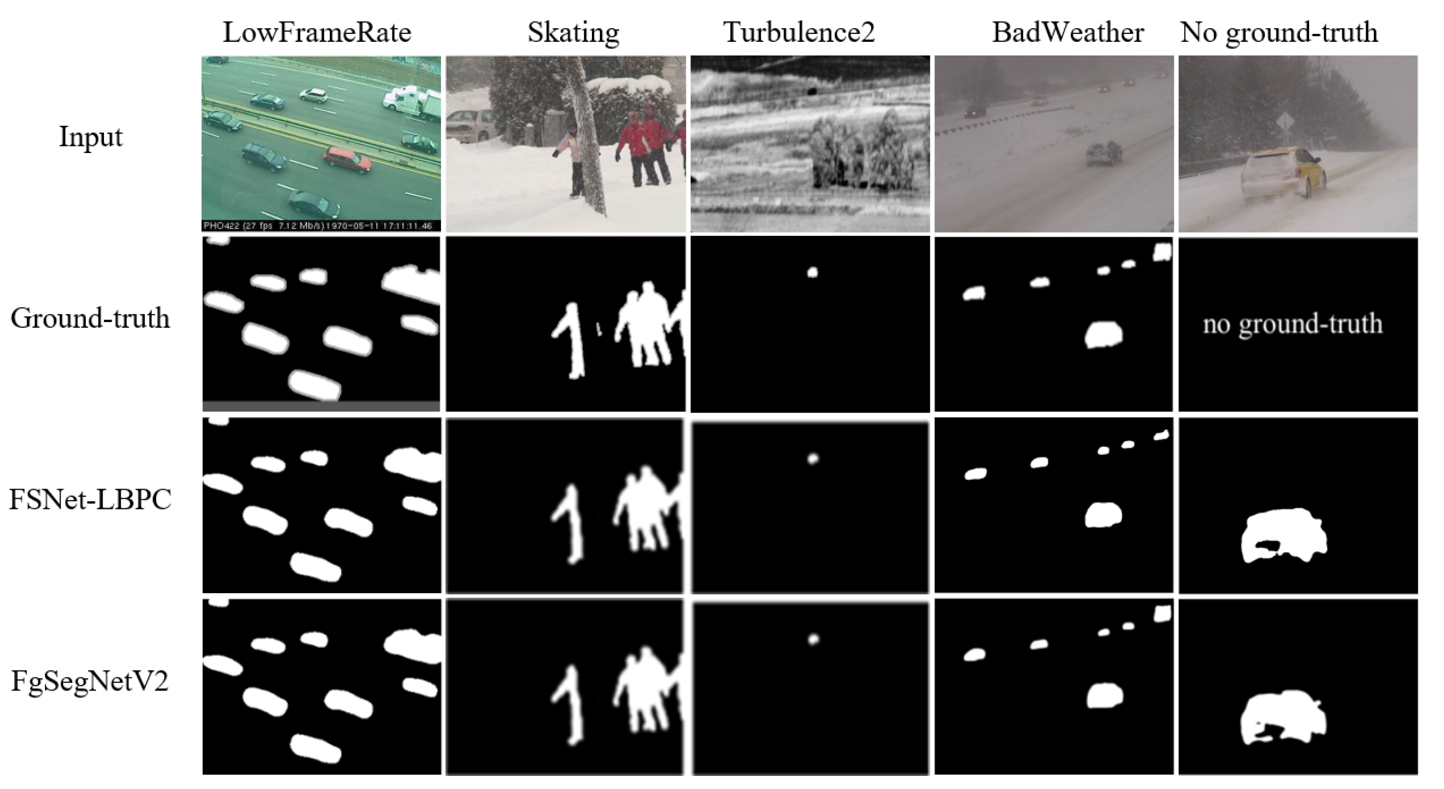
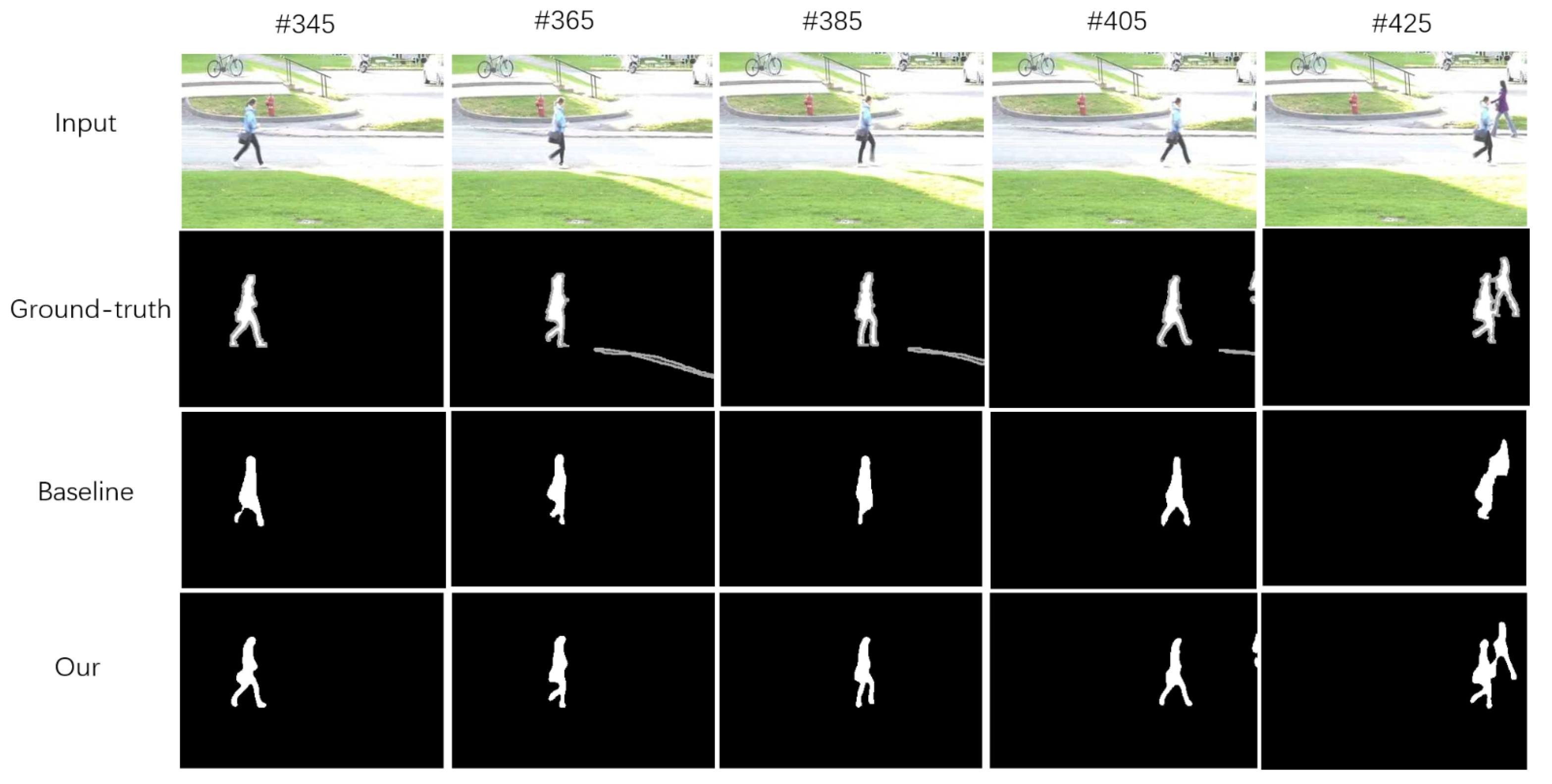
Qualitative Results.Figure 5 (“Input” and “ground truth” adapted from [47]) shows the qualitative results, with several top performance methods taken from the CDNet2014 benchmark [47]. Our MDNet-LBPC detection effect is comparable to similar methods.

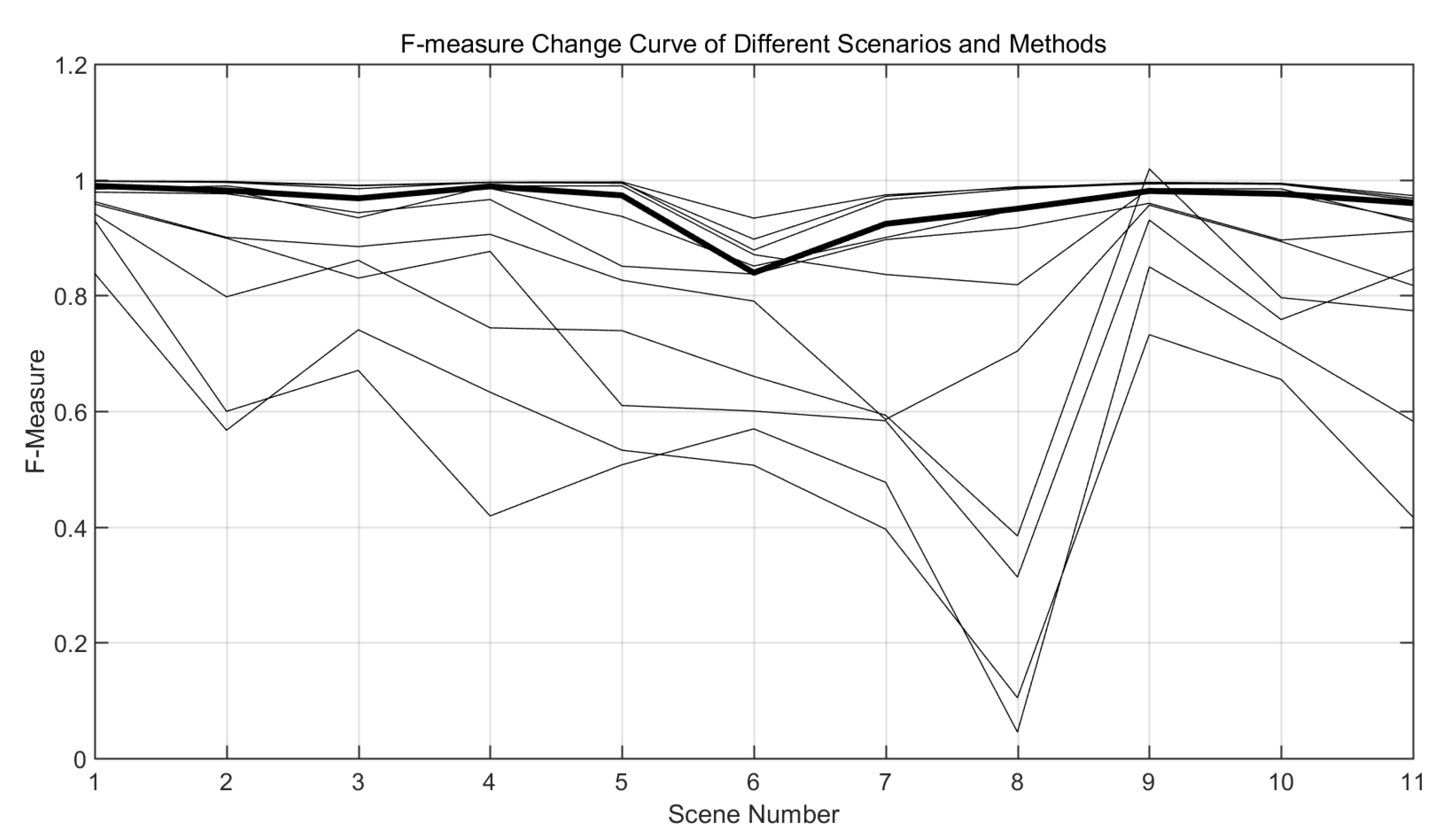
Segmentation Stability Comparison. We used F-measure and classification error percentage (PWC) to analyze the stability performance of 12 methods in each category of the dataset from both positive and negative aspects. First, F is used to evaluate the stability of the model in each category of the data set. The F of each method in each category of the data set is counted, and the curve of its change with the scene is drawn on a graph, as shown in Figure 6. The vertical axis represents F, and the horizontal axis 1 to 11 sequentially represent 11 scenes of CDNet2014 [47].

It can be seen that the curve corresponding to our method is one of the top curves in the whole curve comparison diagram. The model segmentation accuracy belongs to one of the top few methods in the current CDNet2014 [47] data set, indicating that this method has excellent segmentation performance. Compared with the curve at the bottom of the figure (the segmentation accuracy is unstable), the curve corresponding to the model in this paper changes gently, which indicates that our method has good stability for video segmentation of different scenes.

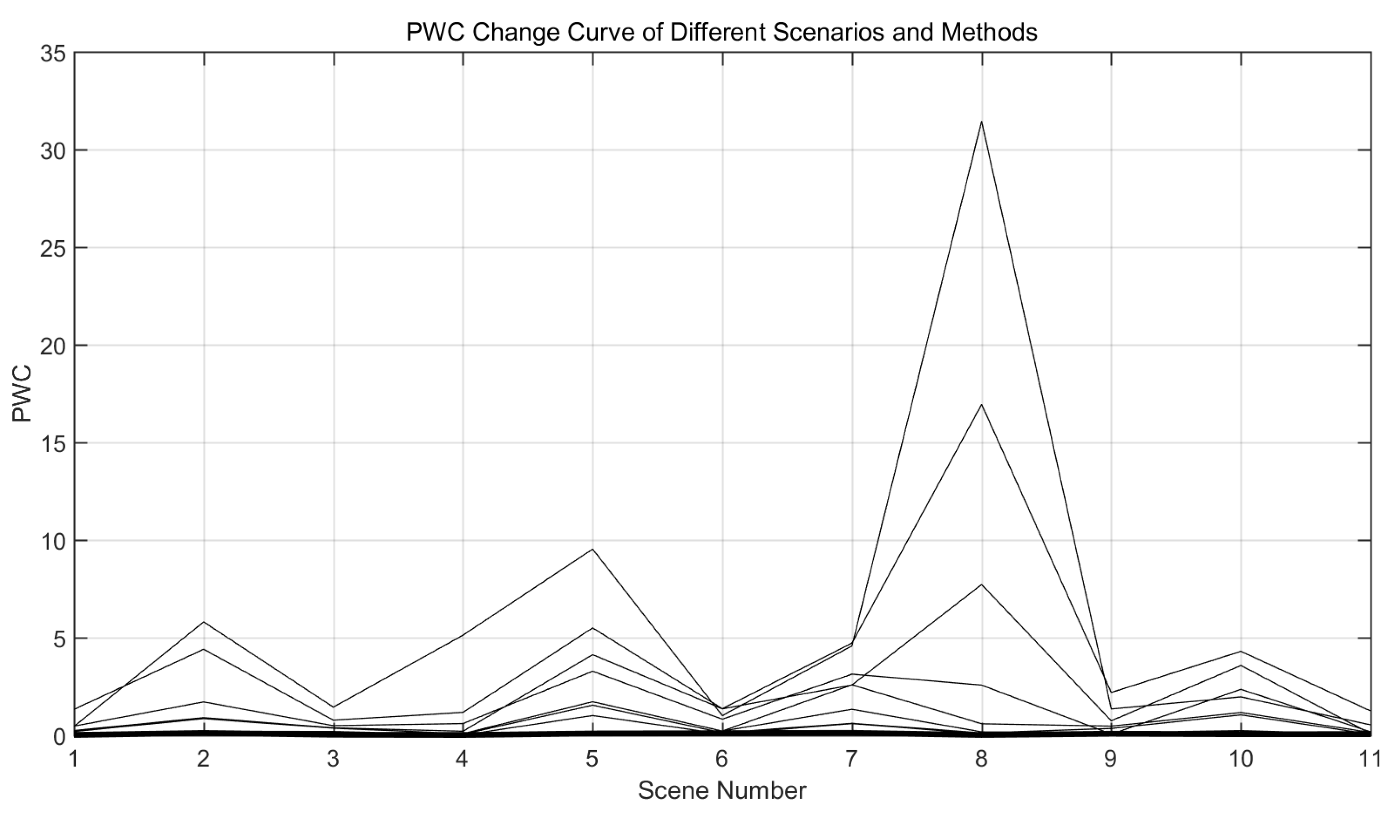
For the percentage of misclassification (PWC), we counted the PWC of each method in each category of the dataset, and plotted its curve with the scene as shown in Figure 7. The vertical axis represents PWC and the horizontal axis represents each scene. It is shown in the figure that among the methods with better performance on the current CDNet2014 [47] data set, the curve corresponding to the method in this paper is one of the lowest ones in the whole curve comparison diagram, indicating that the model segmentation error rate is low and the curve change is also gentle. This proves the segmentation accuracy and stability of the model with respect to classification accuracy. Therefore, the experiment shows that our model not only has high segmentation accuracy, but also has good segmentation stability, and can achieve accurate segmentation of various scenes.

5. Conclusions

In this paper, we have proposed a novel semantic segmentation and lightweight-based method (Real-time Motion Detection Network Based on Single Linear Bottleneck and Pooling Compensation, MDNet-LBPC) for motion detection. In order to improve the efficiency of model inference, we first propose a single linear bottleneck operator to make the lightweight network. In order to handle the problem of information loss due to the use of pooling for the reduction of feature dimensions in the network, we also propose a pooling compensation mechanism to supplement useful information. The experimental results show that, for the segmentation accuracy, it can be seen from Table 8 that our method achieved third place, and each index is close to the method ranking first. For the efficiency of segmentation, this method achieved first place, and the segmentation speed is far ahead of other methods. Specifically, compared with the second-ranking similar method FgSegNet_ V2 [9] our precision (P) has a difference of $1.47\%$, and the segmentation speed has been greatly improved, reaching 151 frames per second.

The proposed real-time unsupervised motion detection network model considers the balance of real-time and accuracy, but it only makes a preliminary lightweight treatment on the network. In actual application, we can prune the network, and compress and accelerate the quantitative model according to specific application scenarios to improve the inference efficiency of the network. Moreover, our research has certain limitations. In the training process, we rely too much on data sets, so we are not completely unsupervised in the real sense. Therefore, in the future work, we can consider how to design a completely unsupervised real-time unsupervised motion detection and segmentation algorithm, so that the model is no longer limited by data set annotation. We expect to further reduce the weight of the model to improve its efficiency.

References

- Zhang, E.; Chen, F. A fast and robust people counting method in video surveillance. In Proceedings of the 2007 International Conference on Computational Intelligence and Security (CIS 2007), Harbin, China, 15–19 December 2007; pp. 339–343. [Google Scholar]
- Yilmaz, A.; Javed, O.; Shah, M. Object tracking: A survey. ACM Comput. Surv. 2006, 38, 13-es. [Google Scholar] [CrossRef]
- Aguilera, J.; Thirde, D.; Kampel, M.; Borg, M.; Fernandez, G.; Ferryman, J. Visual surveillance for airport monitoring applications. In Proceedings of the Computer Vision Winter Workshop, Telc, Czech Republik, 6–8 February 2006; pp. 6–8. [Google Scholar]
- Faktor, A.; Irani, M. Video Segmentation by Non-Local Consensus voting. BMVC 2014, 2, 8. [Google Scholar]
- Wren, C.R.; Azarbayejani, A.; Darrell, T.; Pentl, A.P. Pfinder: Real-time tracking of the human body. Pattern Anal. Mach. Intell. 1997, 19, 780–785. [Google Scholar] [CrossRef]
- Brox, T.; Malik, J. Object segmentation by long term analysis of point trajectories. In Proceedings of the 11th European Conference on Computer Vision, Heraklion, Greece, 5–11 September 2010; pp. 282–295. [Google Scholar]
- Stein, A.; Hoiem, D.; Hebert, M. Learning to find object boundaries using motion cues. In Proceedings of the International Conference on Computer Vision, Rio de Janeiro, Brazil, 14–21 October 2007; pp. 1–8. [Google Scholar]
- Fukuchi, K.; Miyazato, K.; Kimura, A.; Takagi, S.; Yamato, J. Saliency-based video segmentation with graph cuts and sequentially updated priors. In Proceedings of the 2009 IEEE International Conference on Multimedia and Expo, New York, NY, USA, 28 June–3 July 2009; pp. 638–641. [Google Scholar]
- Lim, Long Ang and Keles, Hacer Yalim.: Learning multi-scale features for foreground segmentation. Pattern Anal. Appl. 2020, 23, 1369–1380. [CrossRef]
- Lim, L.A.; Keles, H.Y. Foreground Segmentation Using a Triplet Convolutional Neural Network for Multiscale Feature Encoding. Pattern Recognit. Lett. 2018, 112, 256–262. [Google Scholar] [CrossRef]
- Qiu, M.; Li, X. A fully convolutional encoder–decoder spatial–temporal network for real-time background subtraction. IEEE Access 2019, 7, 85949–85958. [Google Scholar] [CrossRef]
- Tezcan, M.O.; Ishwar, P.; Konrad, J. BSUV-Net 2.0: Spatio-Temporal Data Augmentations for Video-Agnostic Supervised Background Subtraction. IEEE Access 2021, 9, 53849–53860. [Google Scholar] [CrossRef]
- Rahmon, G.; Bunyak, F.; Seetharaman, G.; Palaniappan, K. Motion U-Net: Multi-cue encoder-decoder network for motion segmentation. In Proceedings of the 2020 25th International Conference on Pattern Recognition (ICPR), Milan, Italy, 10–15 January 2021; pp. 8125–8132. [Google Scholar]
- Zheng, W.; Wang, K.; Wang, F.Y. A novel background subtraction algorithm based on parallel vision and Bayesian GANs. Neurocomputing 2020, 394, 178–200. [Google Scholar] [CrossRef]
- Lim, L.A.; Keles, H.Y. Foreground segmentation using convolutional neural networks for multiscale feature encoding. Pattern Recognit. Lett. 2018, 112, 256–262. [Google Scholar] [CrossRef]
- Wang, Y.; Luo, Z.; Jodoin, P.M. Interactive deep learning method for segmenting moving objects. Pattern Recognit. Lett. 2017, 96, 66–75. [Google Scholar]
- Babaee, M.; Dinh, D.T.; Rigoll, G. A deep convolutional neural network for video sequence background subtraction. Pattern Recognit. 2018, 76, 635–649. [Google Scholar] [CrossRef]
- Jiang, S.; Lu, X. WeSamBE: A weight-sample-based method for background subtraction. IEEE Circuits Syst. Video Technol. 2017, 28, 2105–2115. [Google Scholar] [CrossRef]
- Sajid, H.; Cheung, S.C. Background subtraction for static & moving camera. In Proceedings of the 2015 IEEE International Conference on Image Processing (ICIP), Quebec City, QC, Canada, 27–30 September 2015; pp. 4530–4534. [Google Scholar]
- Zivkovic, Z. Improved adaptive Gaussian mixture model for background subtraction. Pattern Recognit. 2004, 2, 28–31. [Google Scholar]
- Zhang, X.; Zhou, X.; Lin, M.; Sun, J. Shufflenet: An extremely efficient convolutional neural network for mobile devices. In Proceedings of the Computer Vision and Pattern Recognition, Salt Lake City, UT, USA, 18–23 June 2018; pp. 6848–6856. [Google Scholar]
- Howard, A.G.; Zhu, M.; Chen, B.; Kalenichenko, D.; Wang, W.; Wey, T.; Andreetto, M.; Adam, H. Mobilenets: Efficient convolutional neural networks for mobile vision applications. arXiv 2017, arXiv:1704.04861. [Google Scholar]
- Chollet, F. Xception: Deep learning with depthwise separable convolutions. In Proceedings of the Computer Vision and Pattern Recognition, Honolulu, HI, USA, 21–26 July 2017; pp. 1251–1258. [Google Scholar]
- Sandler, M.; Howard, A.; Zhu, M.; Zhmoginov, A.; Chen, L.C. Mobilenetv2: Inverted residuals and linear bottlenecks. In Proceedings of the Computer Vision and Pattern Recognition, Salt Lake City, UT, USA, 18–23 June 2018; pp. 4510–4520. [Google Scholar]
- Stauffer, C.; Grimson, W.E. Adaptive background mixture models for real-time tracking. In Proceedings of the Computer Vision and Pattern Recognition, Fort Collins, CO, USA, 23–25 June 1999; Volume 2, pp. 246–252. [Google Scholar]
- KaewTraKulPong, P.; Bowden, R. An improved adaptive background mixture model for real-time tracking with shadow detection. In Video-Based Surveillance Systems; Springer: Boston, MA, USA, 2002; pp. 135–144. [Google Scholar]
- Ghafari, M.; Amirkhani, A.; Rashno, E.; Ghanbari, S. Novel Gaussian Mixture-based Video Coding for Fixed Background Video Streaming. In Proceedings of the 2022 International Conference on Machine Vision and Image Processing (MVIP), Ahvaz, Iran, 23–24 February 2022. [Google Scholar]
- Barnich, O.; Van Droogenbroeck, M. ViBe: A universal background subtraction algorithm for video sequences. Image Process. 2010, 20, 1709–1724. [Google Scholar] [CrossRef]
- Van Droogenbroeck, M.; Paquot, O. Background subtraction: Experiments and improvements for ViBe. In Proceedings of the 2012 IEEE Computer Society Conference on Computer Vision and Pattern Recognition Workshops, Providence, RI, USA, 16–21 June 2012; pp. 32–37. [Google Scholar]
- Hofmann, M.; Tiefenbacher, P.; Rigoll, G. Background segmentation with feedback: The pixel-based adaptive segmenter. In Proceedings of the 2012 IEEE Computer Society Conference on Computer Vision and Pattern Recognition Workshops, Providence, RI, USA, 16–21 June 2012; pp. 38–43. [Google Scholar]
- Alipour, P.; Shahbahrami, A. An adaptive background subtraction approach based on frame differences in video surveillance. In Proceedings of the International Conference on Machine Vision and Image Processing (MVIP), Ahvaz, Iran, 22–24 February 2022; pp. 1–5. [Google Scholar]
- Bianco, S.; Ciocca, G.; Schettini, R. How far can you get by combining change detection algorithms? In Proceedings of the 19th International Conference, Catania, Italy, 11–15 September 2017; Springer: Cham, Switzerland, 2017; pp. 96–107. [Google Scholar]
- Zeng, D.; Chen, X.; Zhu, M.; Goesele, M.; Kuijper, A. Background subtraction with real-time semantic segmentation. IEEE Access 2019, 7, 153869–153884. [Google Scholar] [CrossRef]
- Braham, M.; Van Droogenbroeck, M. Deep background subtraction with scene-specific convolutional neural networks. In Proceedings of the 2016 International Conference on Systems, Signals and Image Processing (IWSSIP), Bratislava, Slovakia, 23–25 May 2016; pp. 1–4. [Google Scholar]
- Gupta, R.; Raghuvanshi, S.S.; Patel, V. Motion Anomaly Detection in Surveillance Videos Using Spatial and Temporal Features. In Proceedings of the 2022 IEEE 7th International conference for Convergence in Technology (I2CT), Mumbai, India, 7–9 April 2022. [Google Scholar]
- Ji, R.; Lin, S.; Chao, F.; Wu, Y.; Huang, F. Deep neural network compression and acceleration: A review. Comput. Res. Dev. 2018, 55, 1871. [Google Scholar]
- He, K.; Zhang, X.; Ren, S.; Sun, J. Deep residual learning for image recognition. In Proceedings of the 2016 IEEE Conference on Computer Vision and Pattern Recognition, Las Vegas, NV, USA, 27–30 June 2016; pp. 770–778. [Google Scholar]
- Han, D.; Kim, J.; Kim, J. Deep pyramidal residual networks. In Proceedings of the Computer Vision and Pattern Recognition, Honolulu, HI, USA, 21–26 July 2017; pp. 5927–5935. [Google Scholar]
- Shen, F.; Gan, R.; Zeng, G. Weighted residuals for very deep networks. In Proceedings of the 2016 3rd International Conference on Systems and Informatics (ICSAI), Shanghai, China, 19–21 November 2016; pp. 936–941. [Google Scholar]
- Huang, G.; Liu, Z.; Van Der Maaten, L.; Weinberger, K.Q. Densely connected convolutional networks. In Proceedings of the Computer Vision and Pattern Recognition, Honolulu, HI, USA, 21–26 July 2017; pp. 4700–4708. [Google Scholar]
- LeCun, Y.; Boser, B.; Denker, J.; Henderson, D.; Howard, R.; Hubbard, W.; Jackel, L. Handwritten digit recognition with a back-propagation network. Neural Inf. Process. Syst. 1989, 2, 396–404. [Google Scholar]
- Zeiler, M.D.; Fergus, R. Stochastic pooling for regularization of deep convolutional neural networks. arXiv 2013, arXiv:1301.3557. [Google Scholar]
- Long, J.; Shelhamer, E.; Darrell, T. Fully convolutional networks for semantic segmentation. In Proceedings of the Computer Vision and Pattern Recognition, Boston, MA, USA, 7–12 June 2015; pp. 3431–3440. [Google Scholar]
- Ronneberger, O.; Fischer, P.; Brox, T. U-net: Convolutional networks for biomedical image segmentation. In Proceedings of the Medical Image Computing and Computer-Assisted Intervention—MICCAI 2015, Munich, Germany, 5–9 October 2015; Springer: Cham, Switzerland, 2015; pp. 234–241. [Google Scholar]
- Simonyan, K.; Zisserman, A. Very deep convolutional networks for large-scale image recognition. arXiv 2014, arXiv:1409.1556. [Google Scholar]
- Chen, L.C.; Papandreou, G.; Schroff, F.; Adam, H. Rethinking atrous convolution for semantic image segmentation. arXiv 2017, arXiv:1706.05587. [Google Scholar]
- Wang, Y.; Jodoin, P.M.; Porikli, F.; Konrad, J.; Benezeth, Y.; Ishwar, P. CDnet 2014: An expanded change detection benchmark dataset. In Proceedings of the Computer Vision and Pattern Recognition Workshops, Columbus, OH, USA, 23–28 June 2014; pp. 387–394. [Google Scholar]
- Deng, J.; Dong, W.; Socher, R.; Li, L.J.; Li, K.; Li, F.-F. Imagenet: A large-scale hierarchical image database. In Proceedings of the 2009 IEEE Conference on Computer Vision and Pattern Recognition, Miami, FL, USA, 20–25 June 2009; pp. 248–255. [Google Scholar]