Article

Identification Approach for Nonlinear MIMO Dynamics of Closed-Loop Active Magnetic Bearing System

Department of Mechanical and Electro-Mechanical Engineering, National Ilan University, Yilan City 26047, Taiwan
Appl. Sci. 2022, 12(17), 8556; https://doi.org/10.3390/app12178556
Submission received: 6 July 2022 / Revised: 21 August 2022 / Accepted: 24 August 2022 / Published: 26 August 2022
(This article belongs to the Special Issue Advanced Materials and Technology Innovation in Machine System)

Abstract

:
A systematic identification approach for the rotor/radial active magnetic bearing (rotor/RAMB) system is presented in this study. First, the system identification of the controller of commercial TMP is undertaken, and the corresponding linear dynamic models are constructed. To perfectly excite the nonlinearities of the rotor/RAMB system, a parallel amplitude-modulated pseudo-random binary sequence (PAPRBS) generator, which possesses the merits of no correlation among the perturbation signals, is employed. The dynamics of the rotor/RAMB system is identified with a Hammerstein–Wiener model. To reduce the difficulty of the identified two nonlinear blocks, the output nonlinear characteristics are estimated prior to the recursive process. Two conventional nonlinear model structures, i.e., NARX and NARMAX, are employed for comparison to verify the effectiveness of the identified Hammerstein–Wiener model. The averaged fit values of the Hammerstein–Wiener model, NARX model, and NARMAX model are 93.25%, 88.36%, and 76.91%, respectively.

1. Introduction

Compared to ball bearings, active magnetic bearings (AMBs) possess the merits of zero ware, energy conservation, and being contactless and lubrication free. Most of all, the stiffness and damping induced by the active magnetic bearings (AMBs) to support the rotor can be adjusted with the aid of controllers for AMBs. The adjustment of the stiffness and damping of the rotor/AMB system enables the rotor/AMB system to pass the critical/resonant speeds of system [1,2,3,4,5] and suppression of vibrations induced by the unbalance mass of rotor [6,7,8,9,10,11,12,13,14,15]. The performance of the rotor/AMB is dominated by the controller of AMB. One of the reliable approaches to developing controllers is to design the controller based on the identified mathematical model of a plant. Hence, the accuracy of dynamic models for the rotor/AMB system is important.
At present, many scholars have proposed numerous methods to identify the parameters or dynamic models of magnetic-bearing systems. Regarding the estimation of the damping and stiffness of the rotor/AMB system, Molina et al. proposed a gray-box modeling procedure to estimate the displacement stiffness and current stiffness of single-axis magnetic bearings [16]. Hua and Ming proposed an online identification method based on the unbalance vibration suppression algorithm to estimate the parameters of the active magnetic bearing [17]. Lauridsen et al. identified the parameters, i.e., current/force factors, displacement/force factors, and time constant of the first order approximation model through the closed-loop identification method and static-loading method [18]. Zhou et al. presented an unbalance response-based method for identifying closed-loop AMB stiffness and damping coefficients [19]. Xu et al. proposed an identification procedure for rotor/active magnetic-bearing dynamics. The model is established with the finite-element method (FEM) and is verified by various experimental rotor unbalance responses [20]. Prasad and Tiwari proposed a gyroscopic dynamic reduction method to identify the speed-dependent parameters of AMBs equipped with a flexible rotor [21].
On the other hand, scholars have proposed various identification procedures to identify the overall rotor/AMB dynamics. Martynenko investigated the nonlinear dynamics of rotor levitated by the passive–active magnetic bearing [22]. Khader et al. established a 2 × 2 MIMO system identification procedure. The resulted model is the combination of both rigid-mode and flexible-mode models [23]. M.H.R.A. Aziz and R. Mohd-Mokhtar proposed a two-stage identification approach with the continuous subspace method to model the MIMO magnetic-bearing system [24]. R. Mohd-Mokhtar and L. Wang proposed an identification approach to model the linear MIMO dynamics of the radial-magnetic-bearing system [25]. To identify more appropriate behaviors of a real rotor/AMB system, the nonlinear auto-regressive methods are applied. Liu et al. identified the model of zero-bias axial magnetic bearing with the NARX (nonlinear autoregressive with external input) neural network [26]. Miranda and Manzano estimated the coefficients of SISO (single-input, single-output) NARMAX (nonlinear auto-regressive moving average with exogenous variables) polynomial model of radial magnetic bearing [27]. Noshadi et al. proposed a genetic algorithms (GA) identification for AMB which can get the global optimum estimation [28].
Since the dynamics of an open-loop active magnetic bearing (AMB) system is inherently unstable, a controller is essential for an AMB system. However, the performance and the dynamics of the AMB system are dominated by the controller. As a result, the accuracy of the identified model employed to design the controller is important. That is, the more informative the system model is, the more suitable the model-based controller can be designed. However, few papers presented identification procedures for nonlinear MIMO dynamics of the closed-loop rotor/AMB system. Moreover, many nonlinear models of AMBs are identified with black-box identification approaches. It is hard to interpret the information from the black-box models. As most of the controllers for AMBs are model-based controllers, this study aims to propose an identification approach to estimate a high-accuracy dynamic model from a MIMO closed-loop system for controller design.

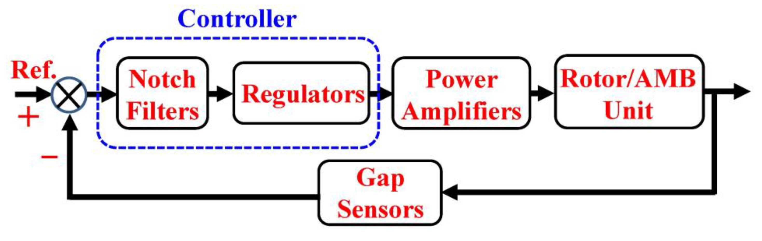
2. System Identification on Controllers for Radial Magnetic Bearings

The system to be identified in this work is the rotor/radial active magnetic bearing (rotor/RAMB) module of the commercial turbo-molecular pump (TMP), OSAKA K701, produced by Osaka Vacuum, Ltd. (Chuo-ku, Osaka). This section is aimed at identifying the controller embedded in the closed-loop TMP system. The control structure of the TMP is depicted in Figure 1. Since the control loop of TMP has integrated: (i) controller, (ii) power amplifier, (iii) shaft/rotor, and (iv) gap sensors, the following steps are to be undertaken so that the transfer function of the controller, G C ( s ) , can be obtained. The identification procedure of the controller is depicted in Figure 2.
Step #1.
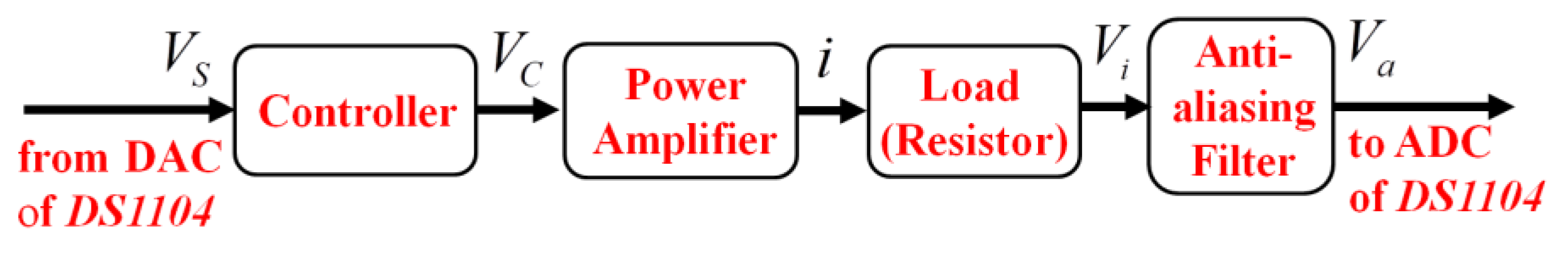
Measure the upper and lower bounds of the control circuit’s input and output signals.
Step #2.
Disconnect the control circuit from the control loop of the TMP, but the power is still supplied to the control circuit.
Step #3.
Excite the control circuit with the ‘chirp’ perturbation signals and record the corresponding responses.
Step #4.
Construct the dynamic model of the controller via the aid of the commercial software, MATLAB.
The internal view of the electronic control unit (ECU) for TMP, Osaka TD700/1100, is shown in Figure 3. The detailed structures of the control circuit of AMBs are depicted in Figure 4. The notations, e.g., S1, S3, …, S9, CP2, CP4, …, CP8 and CP10 are referred to as test points. Embedded in the control circuits, we employ the notch filters to lower down the control force under critical speeds and make the shaft of TMP to spin around its inertia axis instead of its centroidal axis. By applying the notch filters, vibrations induced by the unbalance mass of the rotor can be, to some extent, suppressed.
The individual control circuit for AMBs, composed of resistors, capacitors, and operational amplifiers (Op-Amps), is of the analog type. As a result, the controller can be identified by a linear system approach. In addition, because these five sets of control circuits are not connected to each other, the scheme by linear single-input-single-output (SISO) system identification is employed.
The block diagram of system identification on the controller is depicted in Figure 5. As to the rotor/AMB unit, the load to the power amplifiers is nothing but the AMB coils. Moreover, the AMB coil is of inductive load whose dynamic behavior can be expressed by a first-order equation. To identify the dynamics of the controller, the AMB coils are replaced by resistors whose resistance values are the same as those of the AMB coils. Furthermore, an anti-aliasing filter, i.e., a second-order Butterworth filter, is cascaded ahead of the ADC (analog-to-digital converter) to restrict the bandwidth of the signal to satisfy the Nyquist–Shannon sampling theorem over the band of interest [29]. The test rig for system identification on the controller is shown in Figure 6. To identify the controller, the input signal is the type of chirp in a sinusoidal waveform whose frequency is increased exponentially. The initial frequency of the chirp signal is 0 Hz, and the final frequency is 5000 Hz. The time duration of the chirp signal is set as 10 s, and the sampling period of DS1104, T S , is set as 0.5 ms.

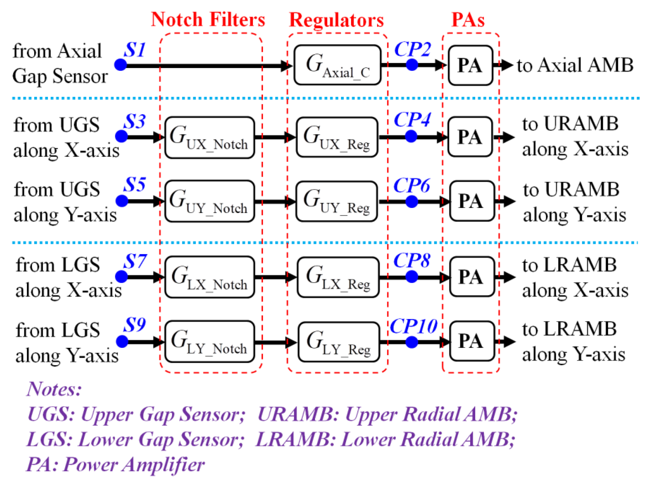
2.1. System Identification on Controllers for URAMB

There are two controllers applied to regulate the position deviations of a rotor by upper radial AMB (URAMB) along the X-axis and Y-axis, respectively. The controller for URAMB along the X-axis, G UX _ C , is composed of a notch filter and a regulator, i.e., G UX _ Notch and G UX _ Reg , respectively, shown in Figure 4. That is, G UX _ C = G UX _ Reg G UX _ Notch . By direction of the signal flow, the notch filter is cascaded ahead of the regulator. To identify the controller for URAMB along the X-axis, the chirp signal is exerted to Point S3, shown in Figure 4, i.e., the output of the upper gap sensor along the X-axis and the corresponding response is recorded at Point CP4, i.e., the output of the regulator for URAMB along the X-axis. The resulting Bode plot of the controller for URAMB along the X-axis is depicted in Figure 7. It is observed that the frequency of the notch filter is around 550 Hz.
The order of the dynamic model of controller for URAMB along the X-axis is 4. The corresponding state space representation and the discrete-time transfer function are summarized as:
A UX _ C = 3072 . 915 1593 . 095 0 0 1593 . 095 3072 . 915 0 0 0 0 635 . 947 3357 . 384 0 0 3357 . 384 635 . 947
B UX _ C = 147 . 249 182 . 816 13 . 242 19 . 935
C UX _ C = 14 . 930 43 . 428 24 . 018 37 . 681
D UX _ C = 0 . 06795
G UX _ C = ( 0 . 06795   z 4 0 . 4431   z 3 + 0 . 9146   z 2 0 . 7769   z + 0 . 2373 ) /   ( z 4 3 . 62   z 3 + 4 . 94   z 2 3 . 009   z + 0 . 6901 ) ,   where   T S = 0.05   ms
Since the purpose of the controller for URAMB along the X-axis is the same as the controller for URAMB along the Y-axis, i.e., to levitate the rotor stably and to suppress the position deviation of the rotor at the position of URAMB at a certain frequency, the Bode plot of the controller for URAMB along the Y-axis is almost the same as Figure 7. On the other hand, the state space representation and the discrete-time transfer function of the controller for URAMB along the Y-axis are listed as:
A UY _ C = 3117 . 165 1570 . 445 0 0 1570 . 445 3117 . 165 0 0 0 0 615 . 177 3332 . 377 0 0 3332 . 377 615 . 177
B UY _ C = 152 . 878 187 . 223 13 . 747 19 . 596
C UY _ C = 15 . 508 43 . 751 24 . 061 37 . 467
D UY _ C = 0 . 06957
G UY _ C = ( 0 . 06957   z 4 0 . 452   z 3 + 0 . 9319   z 2 0 . 7913   z + 0 . 2417 ) /   ( z 4 3 . 619   z 3 + 4 . 936   z 2 3 . 005   z + 0 . 6885 ) ,   where   T S = 0.05   ms

2.2. System Identification on Controllers for LRAMB

Similarly, the controller for lower radial AMB (LRAMB) along the X-axis, G LX _ C , comprises a notch filter and a regulator, i.e., G LX _ Notch and G LX _ Reg , respectively, shown in Figure 4. That is, G LX _ C = G LX _ Reg G LX _ Notch . The chirp signal is externally imported to Point S7 shown in Figure 4, i.e., the output of lower gap sensor along the X-axis, and the corresponding response is recorded at Point CP8, i.e., the output of the regulator for LRAMB along the X-axis. The Bode plot of the controller for LRAMB along the X-axis is depicted in Figure 8. Unlike the notch frequency of the controllers at URAMB, the notch frequency is designed as 446 Hz for the controllers at LRAMB.
Since the order of the dynamic model of controller for LRAMB along the X-axis is 4, the state space representation and its discrete-time transfer function are as:
A LX _ C = 4559 . 940 0 0 0 0 701 . 529 2635 . 884 0 0 2635 . 884 701 . 529 0 0 0 0 25,679 . 137
B LX _ C = 67 . 522 12 . 302 2 . 900 96 . 335
C LX _ CC = 39 . 352 14 . 682 29 . 212 221 . 189
D LX _ CC = 0 . 1937
G LX _ CC = ( 0 . 1937   z 4 1 . 048   z 3 + 1 . 961   z 2 1 . 558   z + 0 . 4515 ) /   ( z 4 2 . 987   z 3 + 3 . 207   z 2 1 . 422   z + 0 . 2055 ) , where   T S = 0.05   ms
On the other hand, the controllers for LRAMB along the X-axis and along the Y-axis are to levitate the lower part of the rotor together; the characteristics of the controller for LRAMB along the Y-axis are similar to those of the controller for LRAMB along the X-axis. The Bode plot of the controller for LRAMB along the Y-axis is close to that of the controller for LRAMB along the X-axis. The identified models of the controller for LRAMB along the Y-axis are:
A LY _ C = 4600 . 290 0 0 0 0 674 . 501 2639 . 121 0 0 2639 . 121 674 . 501 0 0 0 0 24,903 . 283
B LY _ C = 67 . 886 11 . 936 2 . 836 95 . 533
C LY _ C = 39 . 548 14 . 883 28 . 915 213 . 690
D LY _ C = 0 . 1811
G LY _ C = ( 0 . 1811   z 4 0 . 9952   z 3 + 1 . 879   z 2 1 . 502   z + 0 . 437 ) /   ( z 4 2 . 999   z 3 + 3 . 238   z 2 1 . 45   z + 0 . 2138 ) ,   where   T S = 0.05   ms

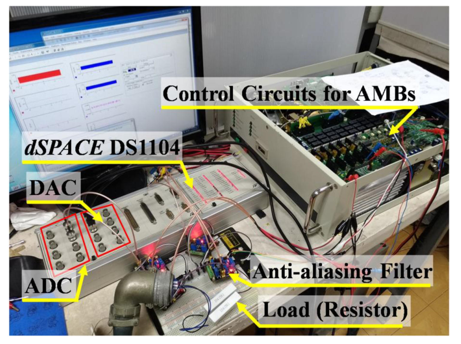
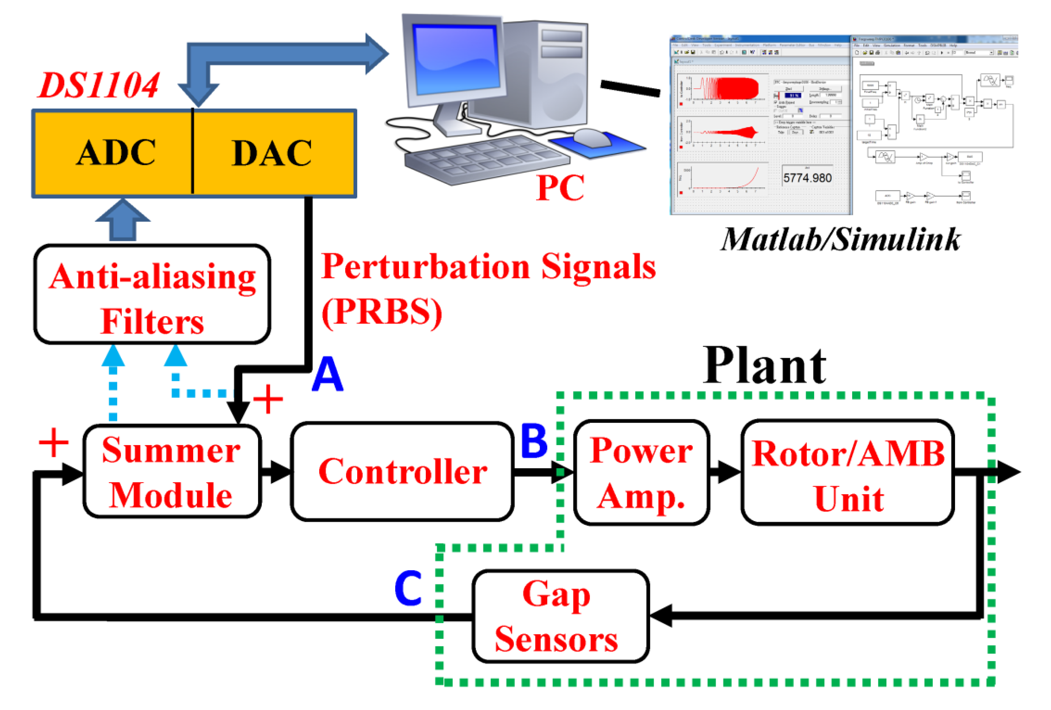
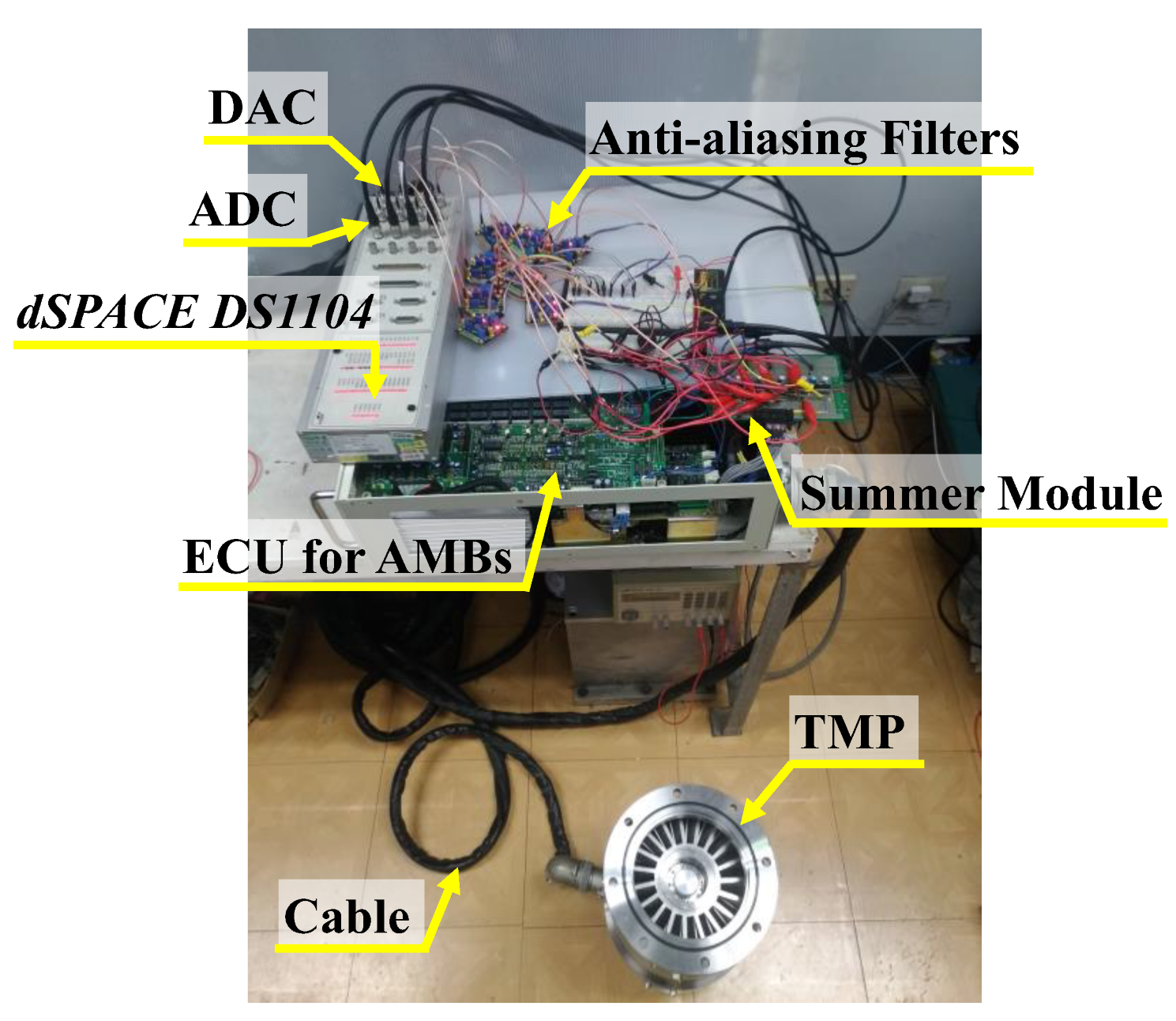
3. Experimental Setup for Identification of Rotor/RAMB Dynamic Model

Because the open-loop dynamics of the rotor/RAMB unit is inherently unstable, the dynamic model of rotor/RAMB unit can be identified accurately as the rotor is fully levitated by the AMBs under the regulation of the controller. To identify the rotor/RAMB dynamic model, the closed-loop system must be excited with the perturbation signals and to record the corresponding responses. However, the circuits of the controller and the power amplifier are firmly connected to each other. As the perturbation signals are directly injected into the closed-loop system without isolation of the impedances at the input points of controller and at the DAC (digital-to-analog converter) of DS1104, the perturbation signals would be distorted. The corresponding terminology of the aforesaid phenomenon is called “loading effects”. To minimize the loading effects, a summer module, shown in Figure 9, is additionally designed by the author and inserted between the gap sensors and the controller in series.

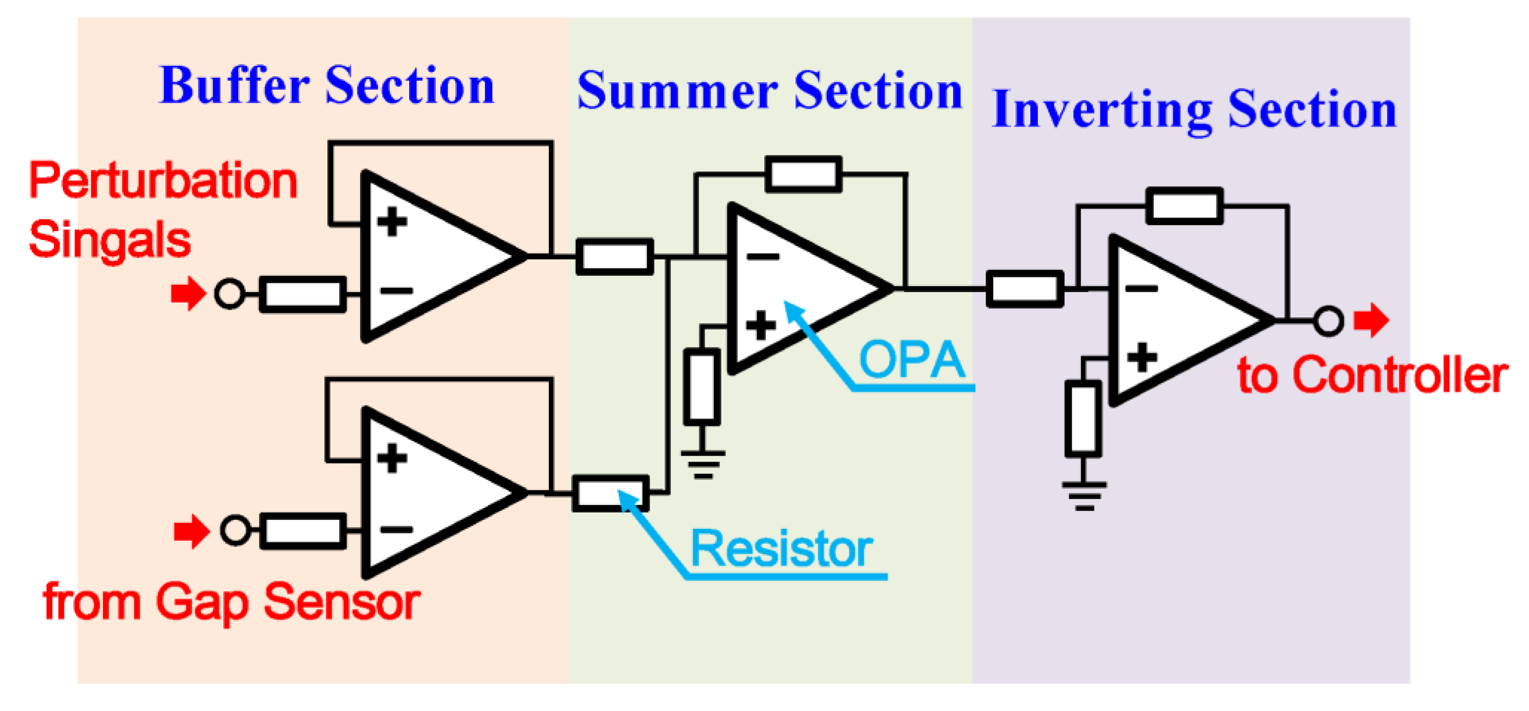
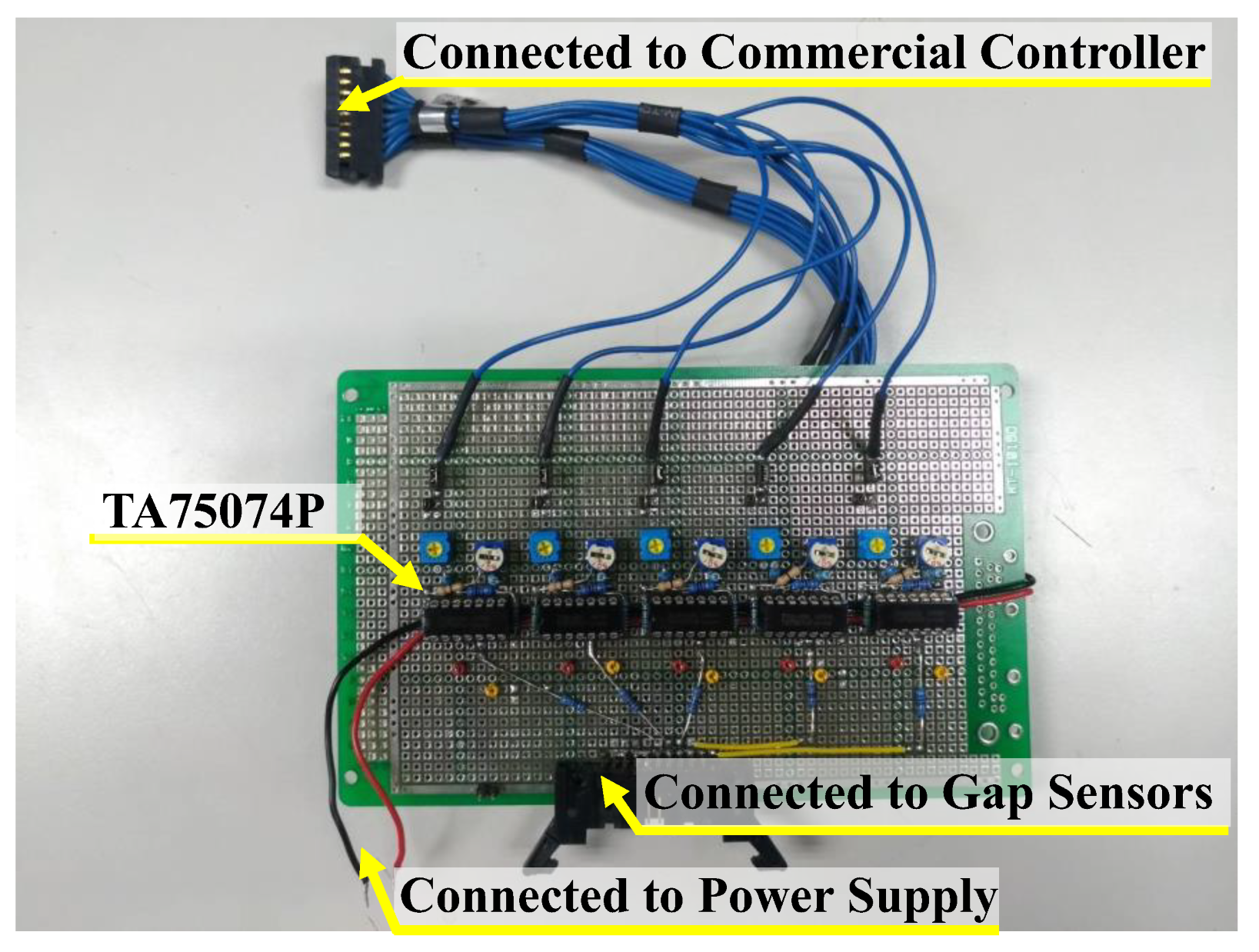
3.1. Design of Summer Module

The layout of the summer module is depicted in Figure 10. The summer module can be divided into three sections: namely buffer section, summer section, and inverting section, respectively. In the buffer section, two voltage followers, namely voltage buffers, are applied to minimize the load effect. Afterwards, one summer is employed to import the perturbation signal into the closed-loop rotor/AMB unit for system identification of the rotor/AMB dynamic system. Finally, a unity-gain inverting amplifier is applied to restore the polarity of the signal processed by the summer module. The photograph of the summer module is shown in Figure 11. The operational amplifier IC, namely, TA74075P, possesses the merits of (i) low-input bias current, (ii) Low-input offset current, (iii) low noise, and (iv) wide bandwidth. Therefore, TA74075P is selected for the summer module.

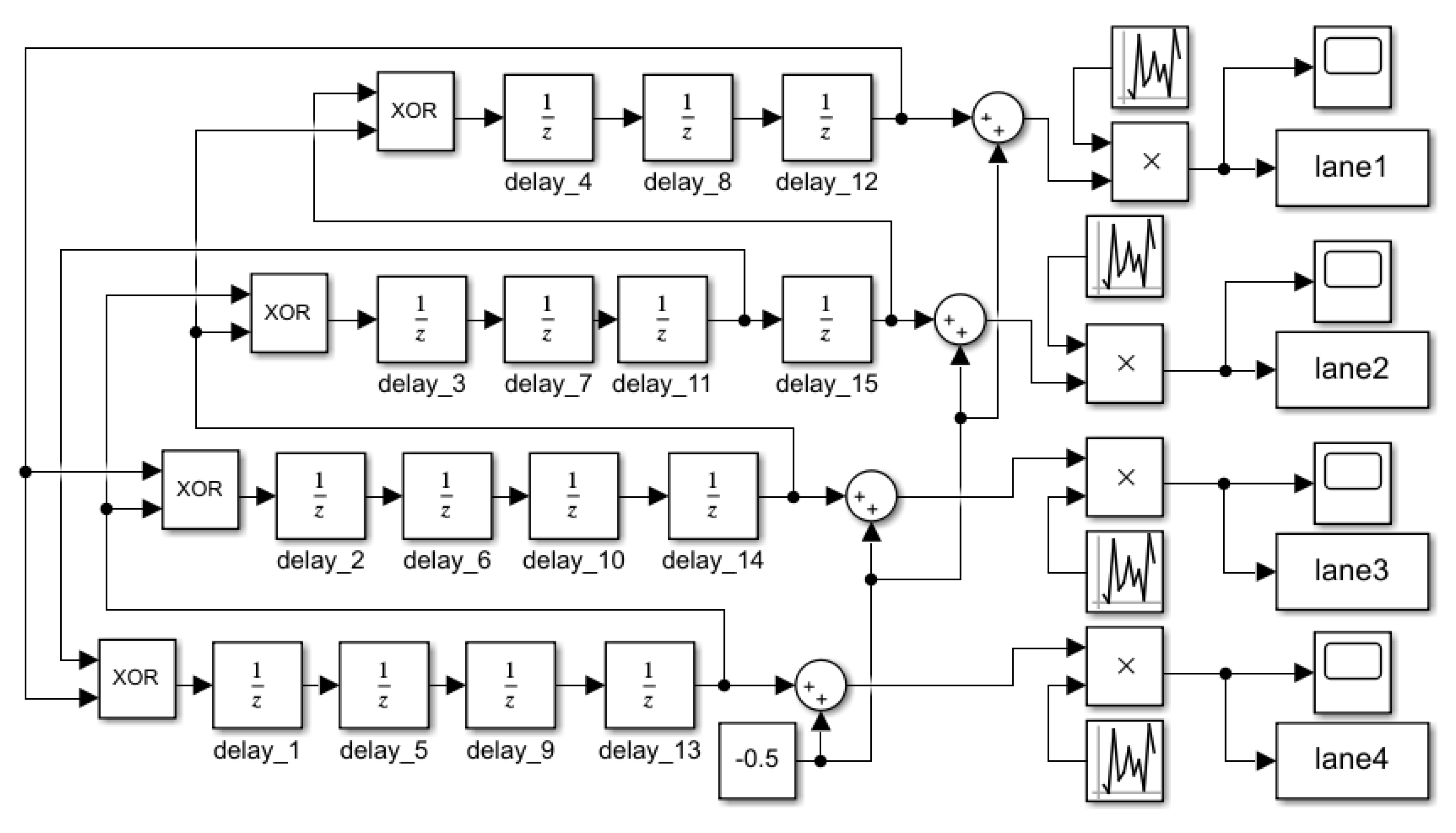
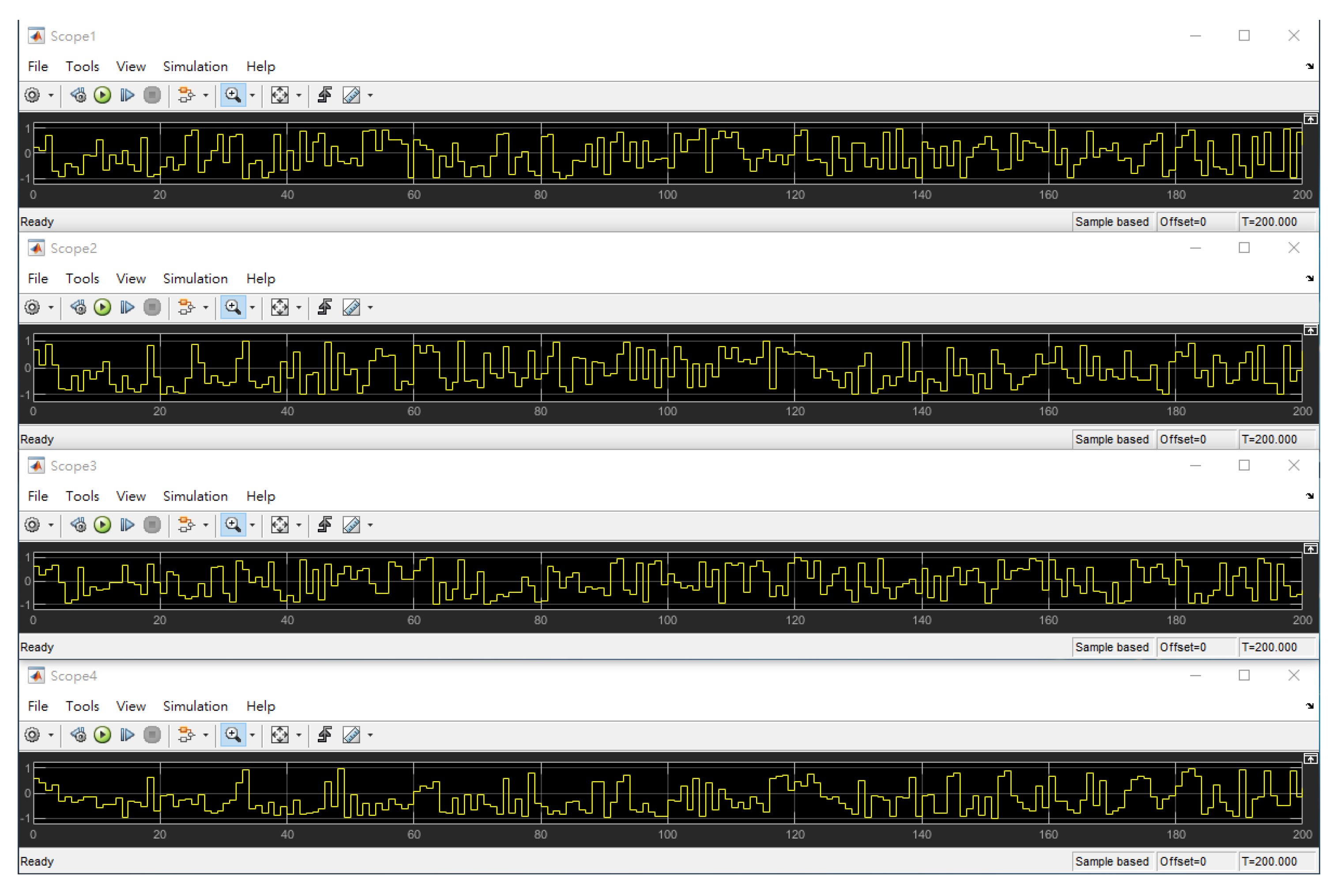
3.2. Parallel Amplitude-Modulated Pseudo-Random Binary Sequence (PAPRBS) Generator

Numerous types of excitation signals can be applied for system identification, e.g., pseudo-random binary sequence (PRBS), chirp signal, multi-sine signal, and stepped sinusoidal wave [30]. It is noted that the rated rotational speed of the TMP rotor is pretty high, e.g., 30,000 RPM for the TMP studied by this work, and the rated speed is higher than the first bending frequency of the TMP rotor. Consequently, the chirp signal is not suitable for system identification upon the rotor/AMB dynamics since the levitated rotor could collide with the auxiliary bearings as the frequency of the perturbation signal is close to/or across the resonance frequencies of the rotor/AMB unit. Among these commonly employed perturbation signals, PRBS, namely maximum length sequence or M-sequence, possesses the merits of deterministic, lowest crest factor and white-noise-alike properties. Therefore, the accuracy of system identification by PRBS can be guaranteed to some extent. In addition, since the system to be identified, i.e., the rotor/RAMB (rotor/radial active magnetic bearing) dynamics, is a MIMO system, the correlation degree between any two perturbation signals has to be reduced as much as possible. Fortunately, once the parallel PRBS generator is well-designed, the aforesaid correlations can be almost eliminated. In this study, hence, the parallel PRBS is adopted as the perturbation signal to identify the MIMO rotor/RAMB dynamic system. Generally, the number of amplitude types of a PRBS is 2, i.e., +V and −V. However, to explore the nonlinear dynamic properties of the rotor/RAMB unit, the amplitude of the perturbation signal has to vary so that the nonlinearities of the studied system, e.g., saturation, hysteresis, or high-order modes, can be appropriately excited. Therefore, in this study, the conventional parallel PRBS generator is extended to a parallel “amplitude-modulated” PRBS (PAPRBS) generator by multiplying a random number sequence. The proposed PAPRBS is designed and realized via the commercial software, Simulink. The layout of the Simulink code for the PAPRBS generator is shown in Figure 12. The order of the PAPRBS is set as 15. As a result, the maximum length of the 15th-order PAPRBS is 2 15 - 1 = 32767 . Four separated sets of perturbation signals can be generated by the PAPRBS generator simultaneously to identify the rotor/RAMB dynamics. To make the four sets of the perturbation signals uncorrelated, the start points of the four sets of perturbation signals are set at: (i) the beginning, (ii) the one-fourth, (iii) the one-half, and (iv) the three-fourth of the 15th-order PRBS, respectively. The length of each perturbation signal sequence is made up by 8000 points such that the correlation between any two perturbation signals can be almost eliminated. The first 200 points of these four perturbation signal sequences are shown in Figure 13. It can be observed that the patterns of these four signals are quite different. To be more specific, the correlations of these four perturbation signals are evaluated and shown in Figure 14. From Figure 14, no cross-correlation between any two of these four perturbation signals is found. It is noted that the bit duration of PAPRBS has to be properly chosen so that the bandwidth of the perturbation signal can cover the operational range of the object/system to be identified. The relation between the maximum frequency of the identified model, i.e., f max , and the bit duration of PAPRBS, i.e., Δ , has to satisfy the following condition [31]:
2 π / 3 Δ > f max
Since the maximum frequency of the identified model of rotor/AMB unit is set as 2000 Hz, the bit duration of PAPRBS signal has to meet the following inequality:
Δ < 2 π / ( 3 * 2000 ) = 1 . 047   ms
Finally, the bit duration is selected as 0.5 ms, and the corresponding period of each PAPRBS as four seconds (i.e., 8000 × 0.5 ms).

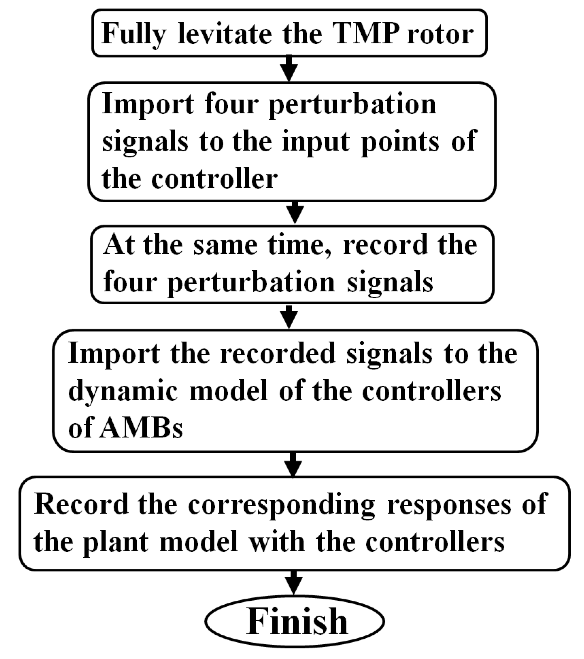
3.3. Parallel Amplitude-Modulated Pseudo-Random Binary Sequence (PAPRBS) Generator
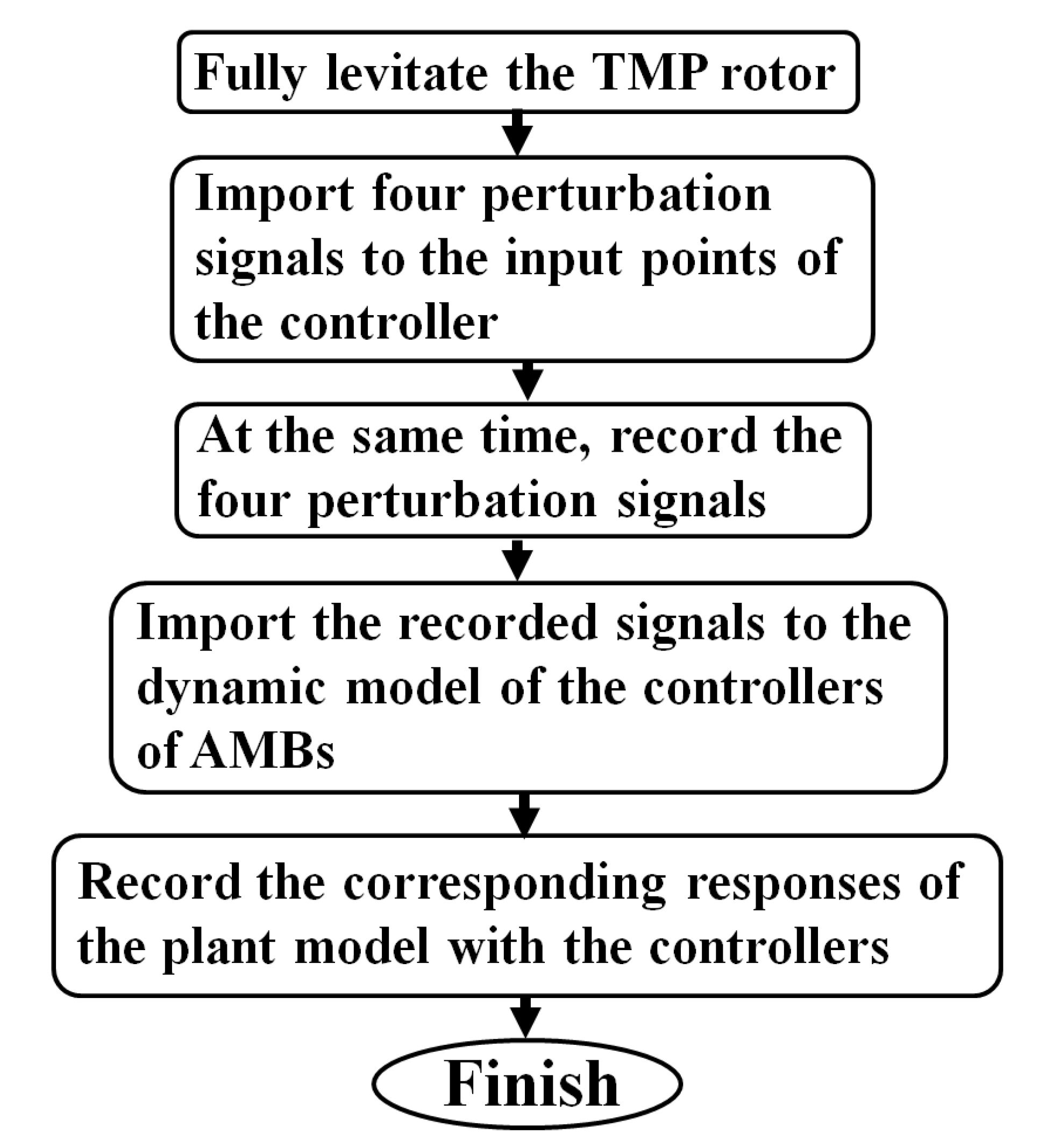
The test rig for the system identification on the multi-input-multi-output (MIMO) rotor/RAMB dynamic system is shown in Figure 15. The corresponding schematic diagram is depicted in Figure 9. In the experiments, the perturbation signals, i.e., PAPRBS signals, are imported to the input points of the controller, i.e., S3, S5, S7 and S9 shown in Figure 4, as the rotor is fully levitated by the commercial controller. Afterwards, the perturbation signals and their corresponding responses, i.e., position deviations of the rotor, are recorded and will be used later.
To construct the rotor/RAMB dynamic model by experiments, the input signals to the plant and the corresponding responses of the rotor/RAMB unit, i.e., Point B and Point C shown in Figure 9, respectively, are necessary to be recorded initially. The plant is referred to as the rotor/RAMB unit in this study. In order not to introduce the noises to the power amplifier directly, the input signals to the plant are not recorded at Point B but at Point A. The detailed steps to generate the corresponding responses at Point B, shown in Figure 9, by applying the perturbation signals recorded at Point A, as shown in Figure 9, to the dynamic model of controllers of AMBs are summarized as:
(i).
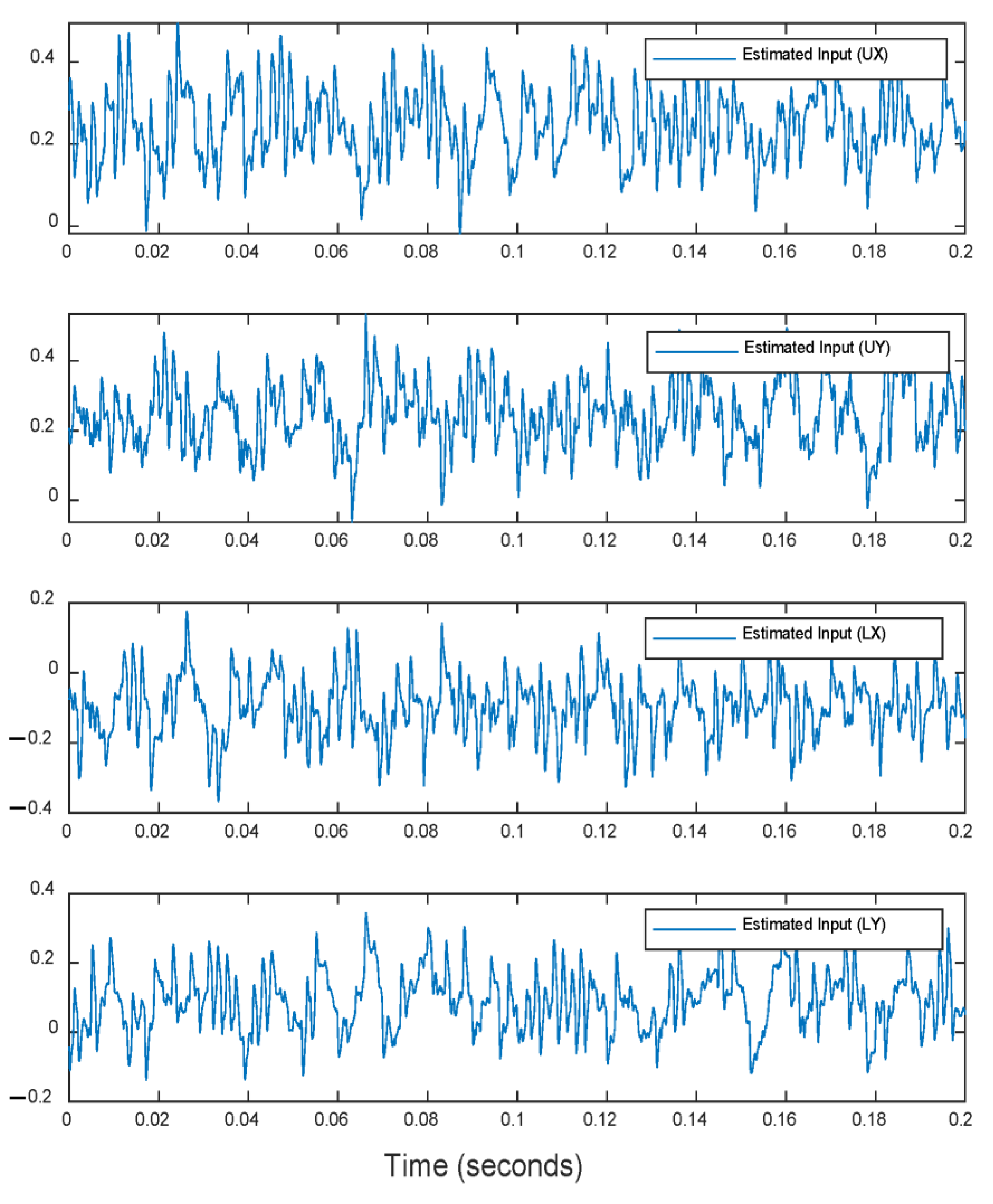
Four perturbation signals are imported at the input points of the controllers, as the TMP rotor is fully levitated.
(ii).
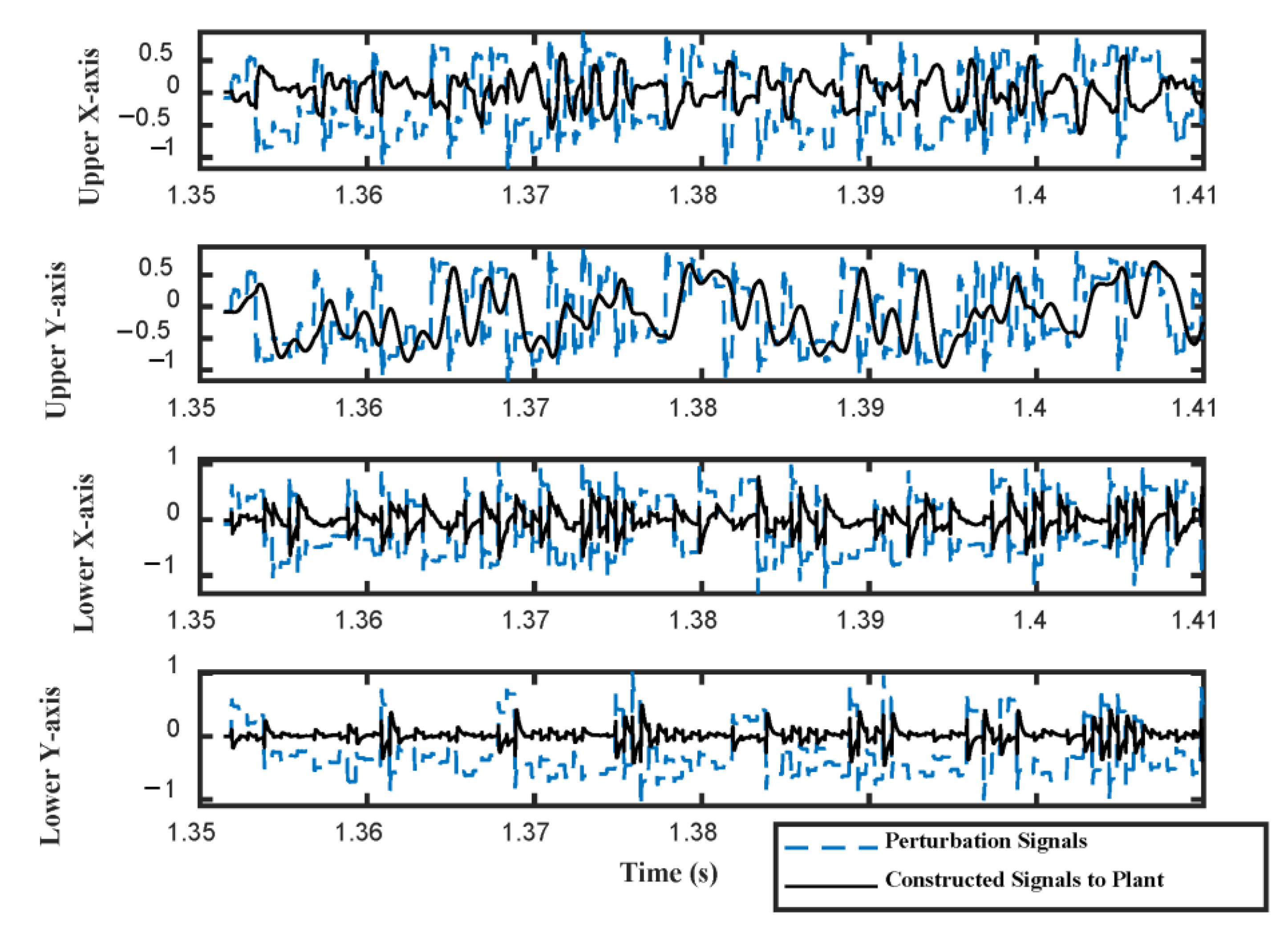
Meanwhile, record the four perturbation signals imported at the input points of the controller, i.e., at Point A, shown in Figure 9.
(iii).
Import the recorded four perturbation signals to the dynamic model of the controllers of AMBs, i.e., Equation (5), Equation (10), Equation (15) and Equation (20), respectively.
(iv).
Record the corresponding responses of the plant model with the controllers.
The flowchart of responses generation with perturbation signals is depicted in Figure 16. The sampling period, T S , is set as 0.05   ms . The input signals imported to the dynamic model of the controllers and the corresponding responses are shown in Figure 17. As the input signals to the rotor/RAMB dynamics and the corresponding responses, i.e., Point B and Point C, shown in Figure 9, respectively, are obtained, the rotor/RAMB dynamic model can therefore be identified.

4. System Identification of Rotor/RAMB Dynamics

The 5-DOF (degree of freedom) rotor/active magnetic bearing (rotor/AMB) unit at TMP can be divided into a 4-DOF rotor/radial active magnetic bearing (rotor/RAMB) module and a 1-DOF rotor/axial active magnetic bearing (rotor/AAMB) module. Except the controller for active magnetic bearings (AMBs), the hardware within a closed-loop AMB system comprises power amplifiers, rotor/AMB module, and gap sensors. Compared with the dynamic responses of the mechanical part, i.e., rotor/RAMB module, the dynamic responses of the power amplifier and the gap sensors are much fast. That is, it is reasonable to describe the input/output characteristics of the power amplifier and the gap sensors with static models in the rotor/AMB system. It is noted that the scheme of the Hammerstein–Wiener model [31] is close to the composition of the hardware within a closed-loop AMB system. Hence, the model of the rotor/RAMB unit is described by a MIMO Hammerstein–Wiener model representation in this study. The schematic diagram of the MIMO Hammerstein–Wiener model is depicted in Figure 18. The MIMO Hammerstein–Wiener model comprises a MIMO nonlinear input element, a MIMO linear element, and several SISO nonlinear output elements. The nonlinearities and the dynamic properties of the rotor/RAMB module can be well described by the combination of the Hammerstein model and the Wiener model.
As to the Hammerstein model, the nonlinear static element, H , is cascaded ahead of the linear dynamic element, L . In contrast, the linear dynamic element, L , is cascaded ahead of the nonlinear static elements, w k ,   k = 1 , 2 , .. , j , in the Wiener model. The nonlinear element of the Hammerstein model, H , is to represent the actuator nonlinearities or any other potential nonlinear effects embedded on the system input side. In comparison, the nonlinear elements of the Wiener model, w k ,   k = 1 , 2 , .. , j , are referred to as the output nonlinearities, which are the nonlinear characteristics of gap sensors in this study. The symbols, U and y k ,   k = 1 , 2 , .. , j , denote the inputs and the outputs of the Hammerstein–Wiener model. The symbols, ω k ,   k = 1 , 2 , .. , j and υ k ,   k = 1 , 2 , .. , j , are the white noises and colored noises, respectively. The relations between the elements of the Hammerstein–Wiener model are summarized as:
X = H ( U ) = U + l = 2 n h a l h l ( U ) ,   w h e r e   U = [ u 1 , u 2 , , u i ] T
V = L · X + N · ϖ = k = 1 n C k z n X / 1 + l = 1 n D l z n + 1 + k = 1 m E k z m ϖ / 1 + l = 1 m F l z m
v k ( t ) = w k 1 ( y k ) = l = 1 n w b k l y k l ( t ) , k = 1 , 2 , , j
where i is the number of inputs, j is the number of outputs, n h is the degree of the nonlinear input functions, and n w is the degree of inverse nonlinear output functions. n is the order of the linear dynamic model, and m is the order of the colored-noise model. a l and b k l are the scale parameters, while C k denotes the parameter matrices. The diagonal parameter matrices, D l , E k , and F l , are represented as:
D l = d 1 l 0 d 2 l 0 d j l ,   w h e r e   l = 1 , 2 , .. , n
E k = e 1 k 0 e 2 k 0 e j k ,   w h e r e   k = 1 , 2 , .. , m
F l = f 1 l 0 f 2 l 0 f j l ,   w h e r e   l = 1 , 2 , .. , m
The Hammerstein–Wiener model is a gray-box model, which processes the merits of the white-box model and the black-box model. To reduce the uncertainties of the Hammerstein–Wiener model but keep the nonlinearities of the dynamic model, we can measure the characteristics of the gap sensors prior to the process of parameter estimation. The parameters of the inverse equations of static nonlinear elements shown in Equation (25) are known. The remaining parameters to be estimated are the part of the Hammerstein model, i.e., Equations (23) and (24). Equations (23) and (24) are organized into one multivariable regression equation system:
V ( t ) = k = 1 n φ d k ( t ) θ d k + l = 1 n h φ a c l ( t ) θ a c l + υ ( t )
where υ ( t ) are the colored noises. Normally, colored-noise terms can be regarded as the white noises filtered with the transfer functions. In this study, the colored-noise is assumed to be the ARMA-type. Therefore, Equation (29) can be represented as the auxiliary model:
V ( t )   = k = 1 n φ d k ( t ) θ d k + l = 1 n h φ a c l ( t ) θ a c l + l = 1 m φ e l ( t ) θ e l + l = 1 m φ f l ( t ) θ f l + ϖ ( t )
where
V ( t ) = v 1 ( t ) v 2 ( t ) v j ( t ) ,
φ d k ( t ) = v 1 ( t k ) 0 v 2 ( t k ) 0 v j ( t k ) ,   k = 1 , 2 , .. , n
θ d k = d 1 k d 2 k d j k T ,   k = 1 , 2 , .. , n
φ a c l ( t ) = h 1 ( U ( t j ) ) T 0 h 2 ( U ( t j ) ) T 0 h i ( U ( t j ) ) T ,   l = 1 , 2 , .. , n h
θ a c l = G l T ( : , 1 ) T G l T ( : , 2 ) T G l T ( : , n ) T T ,   l = 1 , 2 , .. , n × n h
φ e l ( t ) = ω 1 ( t l ) 0 ω 2 ( t l ) 0 ω j ( t l ) ,   l = 1 , 2 , .. , m
θ e l = e 1 l   e 2 l e j l T ,   l = 1 , 2 , .. , m
φ f l ( t ) = υ 1 ( t l ) 0 υ 2 ( t l ) 0 υ j ( t l ) ,   l = 1 , 2 , .. , m
θ f l = f 1 l f 2 l f j l T ,   l = 1 , 2 , .. , m
ϖ ( t ) = ω 1 ( t ) ω 2 ( t ) ω j ( t ) ,
where the vectors G l T ( : , n ) T shown in Equation (35) are extracted from G n × n h = C n a n h . Equation (29) is rewritten in the multivariable linear regression form as:
V ( t ) = φ ( t ) θ + ϖ ( t ) = φ L ( t ) φ N ( t ) θ L θ N + ϖ ( t )
where φ L ( t ) = φ d 1 ( t ) φ d n ( t )   φ a c 1 φ a c n h ( t ) , φ N ( t ) = φ e 1 ( t ) φ e m ( t ) φ f 1 ( t ) φ f m ( t ) , θ L = θ d 1 T θ d n T   θ a c 1 T θ a c n h T T , and θ N = θ e 1 T θ e m T   θ f 1 T θ f m T T . It is noted that the terms shown in Equation (36) and Equation (38) cannot be measured from the dynamic system directly. By applying the following equations, the estimated values of these terms can be derived by [33]:
ϖ ^ ( t ) = V ( t )     φ ( t ) θ = V ( t )     φ L ( t ) φ ^ N ( t ) θ ^ L θ ^ N
υ ^ ( t ) = V ( t )   -   φ L ( t ) θ ^ L
Therefore, the parameters of the MIMO dynamic system can be estimated by the unbiased identification algorithm:
θ ^ ( t ) = θ ^ ( t - 1 ) + K ( t ) V ( t ) φ ( t ) θ ^ ( t - 1 ) ,
K ( t ) = P ( t 1 ) φ T ( t ) φ ( t ) P ( t 1 ) φ T ( t ) + I 1 ,
P ( t ) = I K ( t ) φ ( t ) P ( t 1 ) ,
The products of the parameter matrices, C i   ( i = 1 , , n ) and a ^ l   ( l = 2 , , n h ) , shown in the matrix, θ P , are defined as:
θ P = C 1 T C 2 T C n T a 2 T C 1 T a 2 T C 2 T a 2 T C n T a n h T C 1 T a n h T C 2 T a n h T C n T ,
a = 1 , a 2 , , a n h T ,
C = C 1 T , C 2 T , , C n T T ,
The estimation of C l   ( l = 1 , , n ) , i.e., C ^ l   ( l = 1 , , n ) , can be directly obtained from:
C ^ l = G ^ ( l 1 ) n h + 1 ,   l = 1 , , n
The pseudo inverse of the non-square matrix C shown in Equation (49), i.e., C in Equation (47), can be derived by the Moore–Penrose inverse [34]. Hence, a ^ l   (   l = 2 , , n h ) can be derived by the following equation:
a ^ l = θ P C T , l = 2 , , n h
The flowchart of the identification procedure of the Wiener–Hammerstein model is depicted in Figure 19. The identification procedure is accomplished as the following condition is met:
max i θ ^ i ( t ) θ ^ i ( t - 1 ) / θ ^ i ( t - 1 ) < Δ
The parameter Δ shown in Equation (52) is set as 0.01.
As the perturbations fed in the closed-loop system, the perturbation signals and the responses of the plant, i.e., radial position deviations of the rotor, are recorded. The data length for validation is 4000, which is equivalent to the time length of 0.2 s. First, the estimated controller outputs are generated by feeding the recorded perturbation signals generated by the proposed parallel amplitude-modulated PRBS (PAPRBS) to the controller models presented in Section 2. The corresponding controller outputs are shown in Figure 20. The UX, UY, LX, and LY denote the upper RAMB along the X-axis, the upper RAMB along the Y-axis, the lower RAMB along the X-axis, and the lower RAMB along the Y-axis, respectively.
To verify the effectiveness of the identified Hammerstein–Wiener model, two conventional nonlinear model structures, i.e., NARX and NARMAX, are employed for comparison purposes. The NARX model is constructed by the MATLAB System Identification Toolbox. Both numbers of the delayed outputs, delayed inputs are selected as 4. The nonlinear estimator of NARX is selected as the Sigmoid network. The other nonlinear model for comparison is the NARMAX model with the FROLS (forward regression orthogonal least squares) algorithm [34]. The maximum numbers of the delayed outputs, delayed inputs are both selected as 4, and the maximum delayed noise is selected as 3. After several trials, the minimum number of NARMAX terms is selected as 14. By feeding the inputs to the identified models, shown in Figure 20, the responses of the proposed Hammerstein–Wiener model, NARX model, and NARMAX model are depicted in Figure 21. It is observed that the predicted responses of the Hammerstein–Wiener model show the best fit to the validation data, while the worst case is the NARMAX model. Although the predicted responses of the NARX model shows a good approximation result, the responses by the NARX model sometimes diverge with other sets of validation data.
To quantify the accuracy of the identified models, the following equation applies to evaluate the validation fit:
F i t = 100 % × ( 1 k = 1 N ( y k V a l i d y ¯ V a l i d ) ( y k E s t y ¯ E s t ) 2 y V a l i d y ¯ V a l i d )
where N denotes data length, i.e., 4000. y k V a l i d and y k E s t are the kth validation data and kth identified output, respectively. The upper bar represents the mean values. The fit values are summarized in Table 1. The averaged fit values of the Hammerstein–Wiener model, NARX model, and NARMAX model are 93.25%, 88.36%, and 76.91%, respectively.
The significant limitations of this study are addressed as follows:
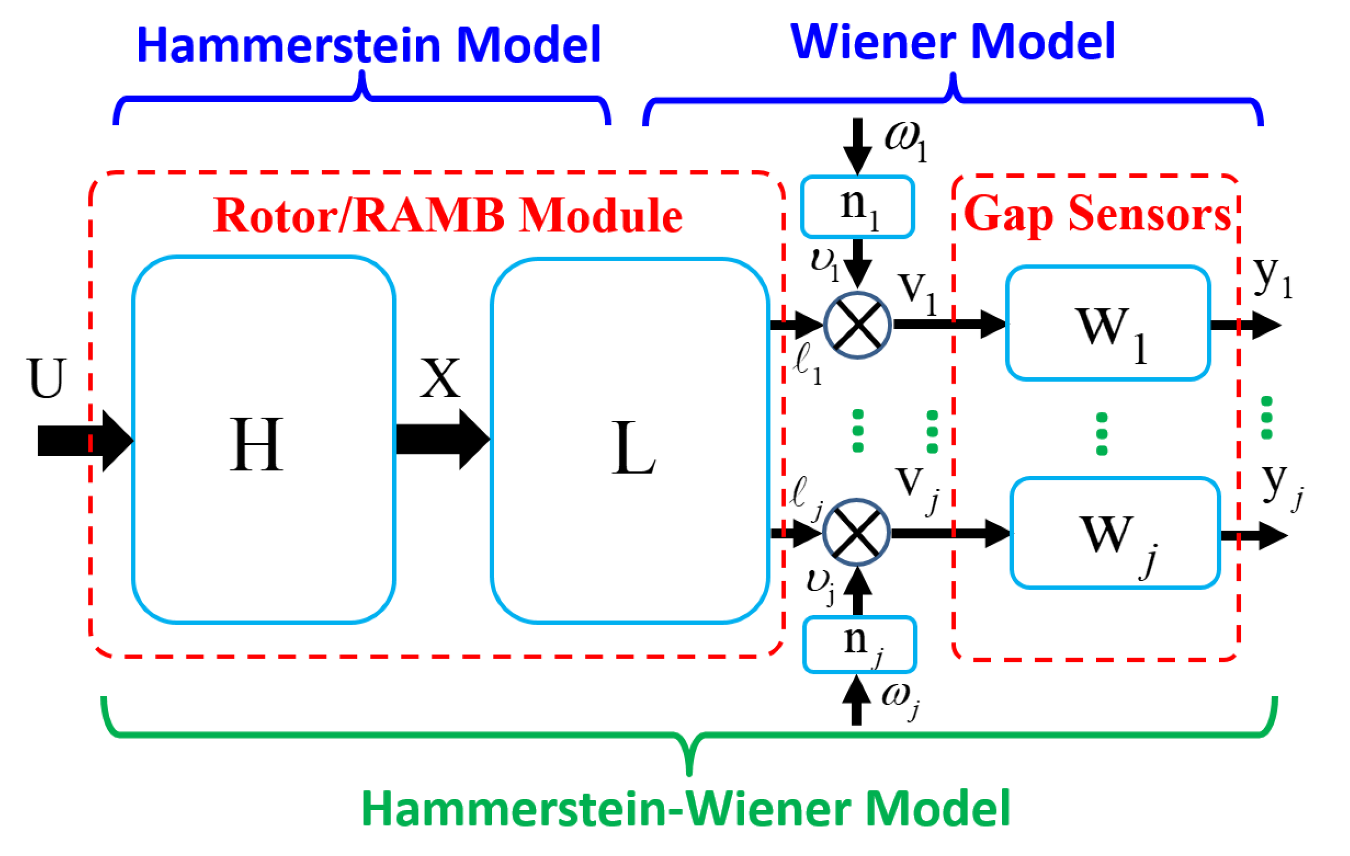
  • By applying the proposed modeling approach presented in Section 4, the mathematical model, i.e., the nonlinear element of the Wiener model, should be estimated prior to the recursive identification algorithm being undertaken. For instance, the static relations between the inputs and outputs of the gap sensor are measured with a high-precision positioning platform.
  • As the perturbation signals are being injected into the rotor/RAMB system, the responses of the rotor/RAMB system will be distorted by the vibrations of the surrounding objects. How the engineering of vibration isolation performs will affect the accuracy of the identified model.

5. Conclusions

In this study, a systematic procedure to identify the nonlinear multi-input multi-output (MIMO) dynamic model from the closed-loop rotor/radial active magnetic bearing (rotor/RAMB) system is proposed. To reduce the potential correlation problem caused by the perturbation signals, a generator of perturbation signals for the MIMO system, named parallel amplitude-modulated pseudo-random binary sequence (PAPRBS), is proposed. By applying the proposed parallel amplitude-modulated pseudo-random binary sequence (PAPRBS) generator, the accuracy of the identified MIMO dynamics can be guaranteed to some extent. Since the composition of the hardware within a closed-loop AMB system is close to the scheme of the Hammerstein–Wiener model, the dynamic behaviors are described as a MIMO Hammerstein–Wiener model by the recursive least squares algorithm. To reduce the difficulty of the identified two nonlinear blocks of the Hammerstein–Wiener model, the output nonlinear characteristics are estimated prior to the recursive process. Two conventional nonlinear model structures, i.e., NARX and NARMAX, are employed for comparison to verify the effectiveness of the identified Hammerstein–Wiener model. The averaged fit values of the Hammerstein–Wiener model, NARX model, and NARMAX model are 93.25%, 88.36%, and 76.91%, respectively. Future work includes development of the online recursive identification algorithm for estimating the nonlinear MIMO dynamics of closed-loop systems.

Funding

This research was partially supported by the Ministry of Science and Technology (Taiwan) with Grant MOST 109-2222-E-197-002-MY3. The author would like to express their appreciations.

Institutional Review Board Statement

Not applicable.

Informed Consent Statement

Not applicable.

Conflicts of Interest

The authors declare no conflict of interest.

References

  1. Saeed, N.A.; Mohamed, M.S.; Elagan, S.K.; Awrejcewicz, J. Integral Resonant Controller to Suppress the Nonlinear Oscillations of a Two-Degree-of-Freedom Rotor Active Magnetic Bearing System. Processes 2022, 10, 271. [Google Scholar] [CrossRef]
  2. Ran, S.; Hu, Y.; Wu, H.; Cheng, X. Active Vibration Control of the Flexible High-speed Rotor with Magnetic Bearings via Phase Compensation to Pass Critical Speed. J. Low Freq. Noise Vib. Act. Control 2019, 38, 633–646. [Google Scholar] [CrossRef]
  3. Zheng, S.; Li, H.; Peng, C.; Wang, Y. Experimental Investigations of Resonance Vibration Control for Noncollocated AMB Flexible Rotor Systems. IEEE Trans. Ind. Electron. 2017, 64, 2226–2235. [Google Scholar] [CrossRef]
  4. Tang, E.; Fang, J.; Zheng, S.; Jiang, D. Active Vibration Control of the Flexible Rotor to Pass the First Bending Critical Speed in High Energy Density Magnetically Suspended Motor. ASME J. Eng. Gas Turbines Power 2015, 137, 112501. [Google Scholar] [CrossRef]
  5. Fang, J.; Zheng, S.; Han, B. AMB Vibration Control for Structural Resonance of Double-Gimbal Control Moment Gyro with High-Speed Magnetically Suspended Rotor. IEEE/ASME Trans. Mechatron. 2013, 18, 32–43. [Google Scholar] [CrossRef]
  6. Zhou, J.; Wu, H.; Wang, W.; Yang, K.; Hu, Y.; Guo, X.; Song, C. Online Unbalance Compensation of a Maglev Rotor with Two Active Magnetic Bearings Based on the LMS Algorithm and the Influence Coefficient Method. Mech. Syst. Signal. Process. 2021, 166, 108460. [Google Scholar]
  7. Gong, L.; Zhu, C. Vibration Suppression for Magnetically Levitated High-Speed Motors Based on Polarity Switching Tracking Filter and Disturbance Observer. IEEE Trans. Ind. Electron. 2021, 68, 4667–4678. [Google Scholar] [CrossRef]
  8. Mao, C.; Zhu, C. Unbalance Compensation for Active Magnetic Bearing Rotor System Using a Variable Step Size Real-Time Iterative Seeking Algorithm. IEEE Trans. Ind. Electron. 2018, 65, 4177–4186. [Google Scholar]
  9. Peng, C.; Sun, J.; Song, X.; Fang, J. Frequency-Varying Current Harmonics for Active Magnetic Bearing via Multiple Resonant Controllers. IEEE Trans. Ind. Electron. 2017, 64, 517–526. [Google Scholar] [CrossRef]
  10. Zheng, S.; Chen, Q.; Ren, H. Active Balancing Control of AMB-rotor Systems Using a Phase-Shift Notch Filter Connected in Parallel Mode. IEEE Trans. Ind. Electron. 2016, 63, 3777–3785. [Google Scholar] [CrossRef]
  11. Chen, Q.; Liu, G.; Han, B. Suppression of Imbalance Vibration in AMB-rotor Systems Using Adaptive Frequency Estimator. IEEE Trans. Ind. Electron. 2015, 62, 7696–7705. [Google Scholar]
  12. Darbandi, S.M.; Behzad, M.; Salarieh, H.; Mehdigholi, H. Harmonic Disturbance Attenuation in a Three-pole Active Magnetic Bearing Test Rig using a Modified Notch Filter. J. Vib. Control 2017, 23, 770–781. [Google Scholar] [CrossRef]
  13. Mu, Y.; Zhou, J.; Di, L.; Zhao, C.; Guo, Q. Active Magnetic Bearing Rotor Model Updating using Resonance and MAC Error. Shock. Vib. 2015, 2015, 263062. [Google Scholar]
  14. Xu, Y.; Zhou, J.; Lin, Z.; Jin, C. Identification of Dynamic Parameters of Active Magnetic Bearings in a Flexible Rotor System Considering Residual Unbalances. Mechatronics 2018, 49, 46–55. [Google Scholar] [CrossRef]
  15. Ranjan, G.; Tiwari, R. On-site High-speed Balancing of Flexible Rotor-bearing System Using Virtual Trial Unbalances at Slow Run. Int. J. Mech. Sci. 2020, 183, 105786. [Google Scholar] [CrossRef]
  16. Molina, L.M.C.; Bonfitto, A.; Tonoli, A.; Amati, N. Identification of Force-Displacement and Force-Current Factors in an Active Magnetic Bearing System. In Proceedings of the 2018 IEEE International Conference on Electro/Information Technology, Rochester, MI, USA, 3–5 May 2018. [Google Scholar]
  17. Hua, L.; Ming, D. Research on Vibration of Magnetic Suspension Rotor System Caused by Magnetic Bearing Model Error-closed-loop Parameter Identification Method. In Proceedings of the 2nd International Conference on Frontiers of Materials Synthesis and Processing, Sanya, China, 10–11 November 2018. [Google Scholar]
  18. Lauridsen, J.S.; Voigt, A.J.; Mandrup-Poulsen, C.; Nielsen, K.K.; Santos, I. Identification of Parameters in Active Magnetic Bearing Systems. In Proceedings of the 15th International Symposium on Magnetic Bearings, Kitakyushu, Japan, 3–6 August 2016. [Google Scholar]
  19. Zhou, J.; Di, L.; Cheng, C.; Xu, Y.; Lin, Z. A Rotor Unbalance Response based Approach to the Identification of the Closed-loop Stiffness and Damping Coefficients of Active Magnetic Bearings. Mech. Syst. Signal Process. 2016, 66, 665–678. [Google Scholar] [CrossRef]
  20. Xu, Y.; Zhou, J.; Di, L.; Zhao, C. Active Magnetic Bearings Dynamic Parameters Identification from Experimental Rotor Unbalance Response. Mech. Syst. Signal Process. 2016, 83, 228–240. [Google Scholar] [CrossRef]
  21. Prasad, V.; Tiwari, R. Identification of Speed-dependent Active Magnetic Bearing Parameters and Rotor Balancing in High-speed Rotor Systems. J. Dyn. Syst Meas. Control 2019, 141, 041013. [Google Scholar] [CrossRef]
  22. Martynenko, G. Application of Nonlinear Models for a Well Defined Description of the Dynamics of Rotors in Magnetic Bearings. EUREKA Phys. Eng. 2016, 3, 3–12. [Google Scholar] [CrossRef]
  23. Khader, S.A.; Liu, B.; Sjöberg, J. System Identification of Active Magnetic Bearing for Commissioning. In Proceedings of the 2014 International Conference on Modelling, Identification & Control, Melbourne, VIC, Australia, 3–5 December 2014. [Google Scholar]
  24. Aziz, M.H.R.A.; Mohd-Mokhtar, R. Identification of MIMO Magnetic Bearing System Using Continuous Subspace Method with Frequency Sampling Filters Approach. In Proceedings of the 37th Annual Conference of the IEEE Industrial Electronics Society, Melbourne, Australia, 7–10 November 2011. [Google Scholar]
  25. Mohd-Mokhtar, R.; Wang, L. System Identification of MIMO Magnetic Bearing via Continuous Time and Frequency Response Data. In Proceedings of the 2005 IEEE International Conference on Mechatronics, Taipei, Taiwan, 10–12 July 2005. [Google Scholar]
  26. Liu, Q.; Wang, L.; Ding, Y. Neural Network Identification of an Axial Zero-Bias Magnetic Bearing. In Proceedings of the International Conference on Intelligent Manufacturing and Internet of Things, Chongqing, China, 21–23 September 2018. [Google Scholar]
  27. Miranda, J.A.; Manzano, E.A. Parametric Identification of an Active Magnetic Bearing System Using NARMAX Model. In Proceedings of the 2020 IEEE XXVII International Conference on Electronics, Electrical Engineering and Computing (INTERCON), Lima, Peru, 3–5 September 2020. [Google Scholar]
  28. Noshadi, A.; Shi, J.; Lee, W.S.; Shi, P.; Kalam, A. Genetic algorithm-based system identification of active magnetic bearing system: A frequency-domain approach. In Proceedings of the 11th IEEE International Conference on Control & Automation (ICCA), Taichung, Taiwan, 18–20 June 2014. [Google Scholar]
  29. Anti-Aliasing Filters and Their Usage Explained, National Instruments Corp. 2019. Available online: http://www.ni.com/zh-tw/innovations/white-papers/18/anti-aliasing-filters-and-their-usage-explained.html (accessed on 6 July 2022).
  30. Vuojolainen, J.; Nevaranta, N.; Jastrzebski, R.; Pyrhonen, O. Comparison of Excitation Signals in Active Magnetic Bearing System Identification. Model. Identif. Control 2017, 38, 123–133. [Google Scholar] [CrossRef]
  31. Vilkko, M.; Roinila, T. Designing Maximum Length Sequence Signal for Frequency Response Measurement of Switched Mode Converters. In Proceedings of the Nordic Workshop on Power and Industrial Electronics, Espoo, Finland, 9–11 June 2008. [Google Scholar]
  32. Bai, J.; Mao, Z.; Pu, T. Recursive Identification for Multi-input-multi-output Hammerstein-Wiener System. Int. J. Control 2017, 92, 1457–1469. [Google Scholar] [CrossRef]
  33. Wang, L.; Ji, Y.; Wan, L.; Bu, N. Hierarchical Recursive Generalized Extended Least Squares Estimation Algorithms for a Class of Nonlinear Stochastic Systems with Colored Noise. J. Frankl. Inst. 2019, 356, 10102–10122. [Google Scholar]
  34. Toutounian, F.; Ataei, A. A New Method for Computing Moore-Penrose Inverse Matrices. J. Comput. Appl. Math. 2009, 228, 412–417. [Google Scholar] [CrossRef]
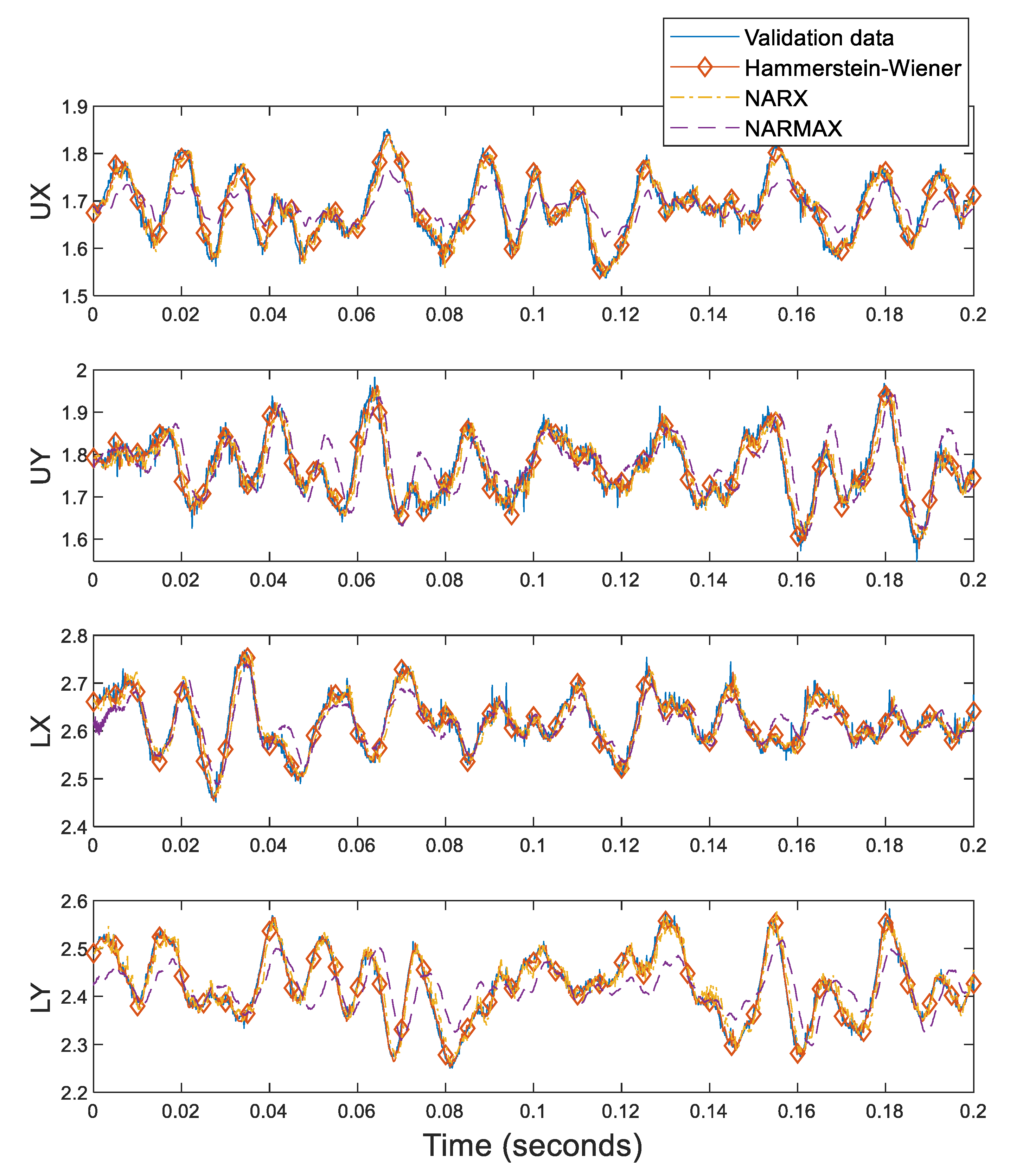
Figure 1. Control structure of rotor/AMB unit.
Applsci 12 08556 g001
Figure 2. Identification procedure of controller.
Applsci 12 08556 g002
Figure 3. Internal view of ECU for TMP (Model: Osaka TD700/1100).
Applsci 12 08556 g003
Figure 4. Detailed structures of the control circuit of AMBs.
Applsci 12 08556 g004
Figure 5. Block diagram of system identification on commercial controller.
Applsci 12 08556 g005
Figure 6. Test rig of system identification on the controller.
Applsci 12 08556 g006
Figure 7. Bode plot of controller for URAMB along the X-axis.
Applsci 12 08556 g007
Figure 8. Bode plot of controller for LRAMB along the X-axis.
Applsci 12 08556 g008
Figure 9. Schematic diagram of experimental setup for identification of rotor/AMB dynamic model.
Applsci 12 08556 g009
Figure 10. Layout of summer module.
Applsci 12 08556 g010
Figure 11. Photograph of summer module.
Applsci 12 08556 g011
Figure 12. Layout of Simulink code for PAPRBS generator.
Applsci 12 08556 g012
Figure 13. First 200 points of PAPRBS.
Applsci 12 08556 g013
Figure 14. Correlations between perturbation signals.
Applsci 12 08556 g014
Figure 15. Test rig for system identification on rotor/AMB dynamics.
Applsci 12 08556 g015
Figure 16. Flowchart of responses generation with perturbation signals.
Applsci 12 08556 g016
Figure 17. Constructed input signals applied to plant.
Applsci 12 08556 g017
Figure 18. Schematic diagram of MIMO Hammerstein–Wiener model for rotor/RAMB dynamics [32].
Applsci 12 08556 g018
Figure 19. Flowchart of identification procedure of Wiener–Hammerstein model.
Applsci 12 08556 g019
Figure 20. Estimated inputs to the rotor/RAMB model for validation.
Applsci 12 08556 g020
Figure 21. Comparison of the proposed Hammerstein-Wiener model, NARX model, and NARMAX model.
Applsci 12 08556 g021
Table 1. Fit values between validation data and responses of Hammerstein–Wiener model, NARX model, and NARMAX model.
Fit (%)Hammerstein–Wiener ModelNARX ModelNARMAX Model
UX92.11%87.63%75.91%
UY93.38%88.88%77.88%
LX91.51%85.57%78.32%
LY95.99%91.34%75.54%
Average93.25%88.36%76.91%
Publisher’s Note: MDPI stays neutral with regard to jurisdictional claims in published maps and institutional affiliations.

