Abstract
In this paper, we present a set of algorithms to enable the development of inexpensive hyperspectral sensors capable of estimating tissue oxygenation for wound monitoring. Estimation is conducted using the extended modified Lambert–Beer law, which has previously been proven robust to differences in melanin concentration. We introduce a novel wavelength selection algorithm that enables the estimation to be performed with high accuracy using only a small number (5–10) of wavelengths. Validation performed with Monte Carlo simulation data resulted in prediction errors <1%, with no significant differences among various skin types, for as few as five wavelengths under conditions representing both high precision instrumentation and more cost-effective sensors designed with inexpensive LEDs and/or filters. Validation with in vivo data collected from an occlusion study with 13 Asian volunteers showed statistically significant separation between the estimates for the at-rest and arterial occlusion states. Additional stability testing proved the proposed algorithms to be robust to small changes in the selected wavelengths as may occur in a real LED due to manufacturing tolerances and temperature fluctuations. This work concluded that the development of an inexpensive hyperspectral device for wound monitoring in all skin types is feasible using just a small number of wavelengths.
1. Introduction
The global prevalence of diabetes among adults was estimated to be 9.5% (537 million people) in 2021 and is expected to rise to 10.2% (578 million people) by 2030 and up to 10.9% (700 million people) by 2045 [1,2]. Of the people diagnosed with diabetes, around 15–25% will develop foot ulcers during their lifetime [3]. These foot ulcers are produced from neuropathy, which leads to the formation of a callus that, as a result of frequent trauma, causes subcutaneous hemorrhage and eventual erosion to an ulcer [4]. In the United States, cost estimates for the management of diabetic foot ulcers are USD 9–13 billion [2,5]. In Nigeria and India, the cost of managing diabetic foot ulcers approaches 4% of the health budget for these countries [6].
Underrepresented communities are particularly at risk. Diabetic diagnosis and its subsequent complications are more prevalent in these underserved populations. African American adults are 60% more likely than non-Hispanic white adults to have been diagnosed with diabetes by a physician and twice as likely as non-Hispanic whites to die from diabetes [7]. According to the Centers for Disease Control and Prevention (CDC), the prevalence of diagnosed diabetes is highest among Native Americans and Alaskan Natives than among any other US racial group [8]. Compounding this, these communities also experience the healthcare difficulties of rural and low-access settings. More than 46 million Americans (15% of the US population) live in rural areas, and this cohort experiences a 17% higher rate of type 2 diabetes than urban residents while simultaneously suffering workforce shortages of primary and specialty care providers [9,10].
The state of wound progression or healing is in large part influenced by the transport of oxygen to the affected area [11]. Tissue oxygenation (SO2), the percentage of oxygenated hemoglobin in the blood, is thus a key indicator of tissue health and a vital metric for monitoring diabetic foot wounds. Hyperspectral imaging (HSI) offers a non-contact, non-invasive method for estimating SO2 in tissue near the affected area, making it an ideal tool for diabetic foot-wound monitoring [12]. Algorithms based on the Lambert–Beer law [13], Kubelka–Munk theory [14], and approximations to the radiative transfer equation (RTE) [15] have been developed to estimate SO2 from hyperspectral information, and many of these algorithms have found their way into clinical devices such as the OxyVu system (Hypermed, MA, USA), the Kent Camera (Kent Imaging, Calgary, AB, Canada), and the TIVITA system (Diaspective, Am Salzhaff, Germany) [16]. However, some researchers have noted disparities in SO2 estimation accuracies for different skin types, with higher errors seen for patients with higher melanin concentration (i.e., darker skin) [17,18,19]. This presents a significant problem for monitoring wound progression in the most-affected populations.
To improve the quality of diabetic foot-wound monitoring for those most in need, including those in rural areas, new cost-effective HSI devices are needed. Such devices must be inexpensive, portable, and robust to differences in melanin concentration. Despite their great promise, current HSI technologies fail to meet most (if not all) of these criteria.
We seek to address these shortfalls by developing new algorithms and methods that will enable the creation of less complex and more accurate wound-monitoring devices. In contrast to typical HSI devices, which collect narrowband information at high resolution (~1 nm), we envision simple devices that collect information at just a small number of wavelengths (~10–15) using inexpensive light-emitting diodes (LEDs) or filters. Not only will the reduction of the number of sampled wavelengths reduce the complexity and cost of these devices, but it will also provide additional benefits such as reduced data collection time, power consumption, and digital storage constraints.
Wavelength selection for hyperspectral technologies is a well-studied problem. Ayala et al. [20] provide a thorough review of the state-of-the-art in wavelength selection algorithms for biomedical imaging applications and offer their own selection algorithm based on a domain adaptation technique. Marois et al. [21] propose a wavelength selection for general chromophore concentration estimation based on a novel nonlinear least squares algorithm, which performs selection by maximizing the singular values of a scattering-modulated absorption matrix. While these techniques have shown high accuracy in tissue oxygenation estimation in general, none of these have focused in particular on the ability to achieve this accuracy across all skin types.
This paper shows proof of concept for a new set of algorithms for selecting narrow wavelengths and estimating SO2 in a cost-effective wound-monitoring device. A new wavelength selection method based on heuristic simulated annealing optimization is introduced. At the core of this optimization is the Extended Modified Lambert–Beer law (EMLB), an SO2 estimation method introduced by Huong et al. [22], which has been proven effective in diabetic wound monitoring [23] and robust to differences in melanin concentration. We reintroduce the EMLB in this work and provide additional details on its implementation. The EMLB is applied with different numbers of selected wavelengths and SO2 estimation accuracy is evaluated with validation datasets consisting of visible-band Monte Carlo simulation spectra representing light to dark skin types, and in vivo spectra collected during an occlusion study from 13 Asian volunteers. To simulate the properties of a collection device designed with inexpensive LEDs and/or filters, these evaluations are repeated with the same data convolved with a 15 nm full-width half maximum (FWHM) Gaussian filter. Furthermore, a stability test is performed to determine the variation in prediction accuracy that might be experienced should the peak wavelengths of the LEDs/filters not match the selected wavelengths, either due to manufacturing tolerances, temperature fluctuations, or other phenomena.
2. Materials and Methods
2.1. Extended Modified Lambert–Beer Law
The Extended Modified Lambert–Beer law (EMLB) was introduced by Huong et al. in [20] to address the deficiencies in the ability of regression models, such as the standard Lambert–Beer law and the Modified Lambert–Beer law, introduced by Twersky [24], to accurately estimate vital parameters including tissue oxygenation (SO2) and percent blood carboxyhemoglobin (COHb). The EMLB has previously been expressed (e.g., [22,25,26]) as:
In this equation, the second term represents the standard Lambert–Beer law, where is the wavelength-dependent absorption coefficient of blood and is the optical path length through the skin. The remaining terms then model artifacts in the absorption spectrum caused by extraneous phenomena. The first term, , provides a constant offset value for the absorbance fit. The combination of these first two terms forms the Modified Lambert–Beer law. The third term is used to model both the scattering effects and absorbance due to melanin in the epidermis, assuming both remain approximately linear over the spectral region of interest. Finally, the last term is used to model the nonlinear effects that arise from complex light scattering and absorption in the dermis.
To better describe how the EMLB is solved to estimate SO2 for a given absorbance spectrum, we rewrite the EMLB as:
Note that the form of the EMLB is modified slightly from its expression in Equation (1) through the inclusion of the parameter, which adds an extra degree of freedom. The solution is then conducted in an iterative two-step manner. In the first step, the MATLAB function fminsearch is invoked to generate candidate values for the parameters , , , , and . These values are then passed to the function that fminsearch has been tasked to minimize. Within this function, the values for the five parameters are set as constants and a linear regression is performed to estimate the values for the regression coefficients . Finally, these regression coefficient values are inserted into Equation (2), and the Euclidian distance between the original spectrum and the EMLB reconstruction is computed and returned to fminsearch. This two-step process continues until either the number of fminsearch iterations exceeds 10,000 or the return value changes by no more than . Bounds for the SO2 estimates were set at 0.0 and 1.0 to prevent physically unrealistic estimates.
2.2. Monte Carlo Simulation
2.2.1. Tools and Datasets
The Monte Carlo simulation is a common method for modeling light-skin interactions. Simulated photons are absorbed and/or scattered probabilistically depending on coefficients determined from the skin model provided by the user. Each simulation run typically accounts for a single wavelength, and the results of multiple runs can be combined to generate a full reflectance spectrum.
One of the most popular Monte Carlo simulation tools is the Monte Carlo for multi-layered tissues (MCML) tool developed by Wang and Jacques [27]. MCML has been used extensively in published studies relating to the optical measurement of skin parameters. Tsumura et al. [28] provide a good description of how the MCML simulation works. Unfortunately, MCML processing is relatively slow given the large number of computations that occur for each simulation. Addressing this key weakness, CUDAMCML was developed by Alerstam et al. [29] to take advantage of the computational acceleration enabled by parallel processing on a graphics processing unit (GPU).
Two separate simulation datasets were developed for this project. The first was used exclusively by the simulated annealing algorithm for wavelength selection (see Section 2.4). It consisted of 36 simulated spectra from 450–800 nm at 1 nm resolution with parameters as given in Table 1. The parameter values were selected to represent typical values for human skin and melanin concentrations in light-skinned adults, moderately pigmented adults, and darkly pigmented adults [30]. These parameters are discussed further in Section 2.3.

Table 1.
Parameters for simulated dataset used in wavelength selection.
The second simulation dataset was used for the validation of the wavelength selection and SO2 estimation algorithms and consisted of 1000 spectra, again from 450 to 800 nm at 1 nm resolution. These spectra were generated using the same parameters as those given in Table 1, except the values for SO2 and were selected at random from a uniform distribution bounded by the maximum and minimum values in Table 1.
2.2.2. Simulation of Data Collection from an Inexpensive HSI Device
The data simulation approach of CUDAMCML effectively assumes a perfect sensor capable of collecting spectral information at precisely known wavelengths with an infinitely narrow bandwidth. This assumption is a poor one for real devices and is particularly poor for a device that relies on inexpensive LEDs and/or filters with relatively wide bandwidths for spectral data collection. Table 2 gives peak tolerance and spectral widths, for example, narrowband LEDs in the 520–600 nm range. Thus, to model a more realistic device, the analysis was repeated with a copy of the simulation dataset where the spectra were convolved with a 15 nm FWHM Gaussian filter using the Python function gaussian_filter1d from the scipy library [31]. Importantly, the absorption coefficients for oxygenated and deoxygenated blood were also convolved with the same filter to produce revised coefficients in a manner similar to the integrated absorption technique [32].
Table 2.
Example visible band LEDs in the 520–600 nm range of interest. Spectral widths are provided as FWHM.
Figure 1a shows the smoothing effect of the Gaussian convolution on an example spectrum. The convolution tends to flatten and broaden the two peaks that result from oxyhemoglobin absorption. This effect is not modeled in the EMLB, so to compensate, we convolve the extinction coefficients for oxy- and deoxyhemoglobin with the same 15 nm Gaussian filter. Figure 1b,c show these coefficients before and after the convolution. Analyses were conducted on the data both before and after convolution to evaluate the differences in performance that might be expected between a costly medical- or industrial-grade instrument and the sort of less expensive device that could benefit patients in poor and rural areas. We refer to analyses with the original data (i.e., before convolution) as the “ideal” case and with the convolved data as the “convolved” case.
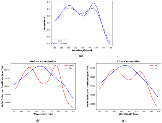
Figure 1.
Effects of convolution with a 15 nm FWHM Gaussian filter. (a) Example spectrum before and after convolution. The other plots show molar extinction coefficients for oxy- and deoxyhemoglobin (b) before and (c) after convolution. Convolution flattens and broadens the distinctive peaks in the oxyhemoglobin curve, most significantly in the higher wavelength lobe, bringing it closer to the deoxyhemoglobin curve.
2.3. Skin Model
Both Monte Carlo datasets were created using a two-layer skin model similar to the one proposed by [15], with an epidermis thickness of 60 μm [30] and a dermis thickness of 2 mm. This model matches the one proposed by Binzoni et al. and is consistent with the approximate maximum penetration depth of visible light in skin [37]. The upper layer is assumed to contain only melanin with volume fraction and the lower layer to contain only blood with volume fraction . Other skin contents (e.g., water and fat) are ignored, since their absorption coefficients are orders of magnitude lower than those of melanin and hemoglobin in the 520–600 nm range of interest [38].
The absorption coefficients for 100% melanin in the epidermis layer are given by Meglinski and Matcher [39] as:
where the wavelength, λ, is in nanometers. These values are multiplied by to arrive at the actual absorption of light in the epidermis. The value of can range from 1.3% to 6.3% for light-skinned adults, 11% to 16% for moderately pigmented adults, and 18% to 43% for darkly pigmented adults [30]. Absorption in the dermis is modeled as a combination of absorption by deoxyhemoglobin (Hb) and oxyhemoglobin (HbO2):
where and are the absorption coefficients for Hb and HbO2, respectively, given by Prahl [40], and and are the concentrations of these two substances in the blood. This equation can be expressed in a more convenient form that clearly illustrates the role of SO2 in the absorbance:
where T is the total concentration of hemoglobin in the blood and .
Scattering coefficients, the same used for both the epidermis and the dermis, are provided by Stavaren et al. [41] based on experimentation with intralipid 10%. These values were found to closely match the scattering behavior of biological tissues found by Bashkatov et al. [42]. Figure 2 shows the absorption and scattering coefficients plotted as functions of wavelength over the visible range. Anisotropy factors, also provided by Staveren et al. [41], are computed as:
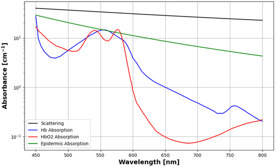
Figure 2.
Scattering and absorption coefficients for the skin model used in this study.
Given the small variation in the wavelength over the range of interest, the index of refraction was set to a constant 1.4 for both layers [22,43].
2.4. Simulated Annealing Wavelength Selection
Instead of sensing the full-resolution visible absorbance spectrum at 450–800 nm, the proposed method uses just a small number of narrow wavelength bands (referred to simply as “wavelengths” in this paper) that are specifically chosen from the vicinity of the hemoglobin peaks (520–600 nm) to yield accurate SO2 estimates using the EMLB. Wavelength selection is accomplished via simulated annealing, a heuristic optimization method modeled after the metallurgical annealing process in which the metal undergoes controlled cooling to remove defects and toughen it. The simulated annealing algorithm consists of a discrete-time inhomogeneous Markov chain with current state and a cooling schedule defined by a starting temperature, , a final temperature, , and a total number of steps, n [44]. The goal of the algorithm is to determine the minimum of a user-defined energy function, .
At each iteration , a new trial state is determined by randomly selecting a “neighbor” of the previous state and calculating its energy. If the resulting energy is lower than the energy from the previous iteration, the trial state becomes the new state of the system. If the resulting energy exceeds the energy of the previous iteration, the algorithm adopts the trial state, with the probability given by:
where is the temperature at iteration i. Note that this equation allows the algorithm to occasionally accept states that result in an increase in energy. This can benefit the optimization by preventing it from becoming stuck in local minima. The probability of accepting such states is high at the beginning of the process when the temperature is high, but gradually decreases with decreasing temperature. The output of the algorithm is the state with the lowest energy encountered throughout the annealing schedule. Figure 3 provides a summary of this algorithm.
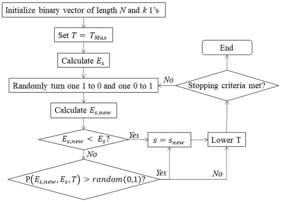
Figure 3.
Flowchart for the simulated annealing algorithm used to select the best k wavelengths for SO2 estimation.
For this wavelength selection problem, the state is defined as an array of binary elements indicating the presence or absence of each wavelength in the full-resolution spectrum. A limit, k, is set on the number of wavelengths selected, such that:
Under this restriction, the state for each iteration is updated by generating a “neighbor” of the current system state. This is done by randomly deselecting one wavelength index from the current state and selecting a new one. The energy of the trial state is then calculated as the average absolute prediction error over the Monte Carlo dataset.
The MATLAB function simannealbnd served as the basis for the implementation of the proposed simulated annealing algorithm. The initial temperature was set to and the maximum number of iterations was set to . The number of steps was chosen to balance the desire for rapid processing with the need for algorithm convergence. The temperature function was modified to allow for a slower cooling rate than the default, and is given by:
where iter is the current number of iterations. With these settings, the probability of acceptance for a 1% increase in the RMSE remained above 66% for the first half of the total iterations, allowing for a less restricted random walk through the solution space. In the latter half of the iterations, the acceptance probability was allowed to drop well below 1%, enabling a more targeted search near the optimal point. After 750 iterations, was increased to 5 and an offset was applied to the number of iterations in the exponent of Equation (3) to reset the cooling rate from that point. The acceptance function was modified to implement the exponential function in Equation (1). After every 100 iterations, the state was returned to the state with the lowest error found thus far to ensure that the algorithm does a thorough search in the area of the state space, which is presumably near the global minimum. The algorithm ended its search upon reaching the maximum number of iterations, or upon reaching 300 consecutive iterations with no change in the average prediction error greater than , whichever came first.
Wavelength selections were conducted for numbers of wavelengths k = 3, 5, 7, 11, 15, 20, 40, and 60 (the total number of wavelengths to select from in the 520–600 nm range was 81). To prevent the unnecessary selection of adjacent wavelengths for low values of k, a validity check was added to the simulated annealing algorithm, whereby a candidate selection was declared invalid if the separation between any pair of wavelengths was less than 2 nm and k < 20.
2.5. Validation Datasets
A two-part validation of the proposed wavelength selection and SO2 estimation algorithm set was performed. The first part evaluated the algorithms’ performance against a Monte Carlo validation dataset that was generated with CUDAMCML using the skin model described in Section 2.3. This simulation dataset, described in Section 2.2, enabled a direct evaluation of SO2 prediction accuracy, since the true SO2 value was known. Validation was performed both on the full 1 nm resolution simulation data to represent the ideal case described in Section 2.2, and on a version of the same data convolved with a 15 nm FWHM Gaussian filter to represent the convolved case.
The second part of the validation process was performed on the in vivo dataset described in [25], which consists of reflectance data collected from 13 Asian volunteers (aged 24.3 ± 2 years). A 9 W white light-emitting diode (LED) (Lumileds, Philips, Schiphol, The Netherlands) illuminated the right index finger of each volunteer from an 80 mm distance at an angle of 20° from normal. An optical fiber connected to a spectrometer (Ocean Optics USB4000) was placed 8 mm from the fingertip at 15° from normal and collected reflectance data at a spectral resolution of 0.2 nm in the wavelength range of 200–850 nm. These data were then converted from reflectance to absorbance, the 520–600 nm wavelength range was extracted, and the resolution was adjusted to 1 nm via cubic interpolation.
2.6. Stability Testing
Additionally, we conducted a series of stability tests where the selected wavelengths were adjusted randomly by ±1 nm to simulate uncertainty in the peak wavelengths. Specifically, for each iteration, a random subset of the k-selected wavelengths was chosen and each peak wavelength in the subset was moved at random by either +1 nm or −1 nm. The goal of this stability testing was to evaluate the sensitivity of our proposed SO2 estimation method to uncertainties in the spectral parameters of our hypothesized inexpensive device.
3. Results and Discussion
3.1. Wavelength Selection
The wavelength selections for various numbers of selected wavelengths, k, for both the ideal case and the convolved case, are shown in Figure 4. Notice that while the selections for the ideal case include both lobes of the oxygenated hemoglobin extinction coefficient curve, the selections for the convolved case tend to favor the left lobe only. This can be explained by observing the effect that the convolution has on the spectra, as shown in Figure 5. Selected wavelengths for k = 5, 6, and 7 are given in Table 3.
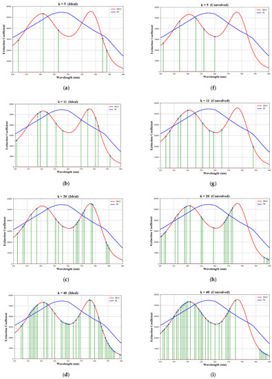
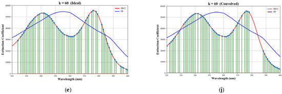
Figure 4.
Wavelength selections for various values of k. The left column shows selections for the ideal case and the right column shows selections for the convolved case. (a,f) k = 5, (b,g) k = 11, (c,h) k = 20, (d,i) k = 40, (e,j) k = 60. The selections are superimposed on plots of the absorption coefficients for oxygenated (red) and deoxygenated (blue) hemoglobin.
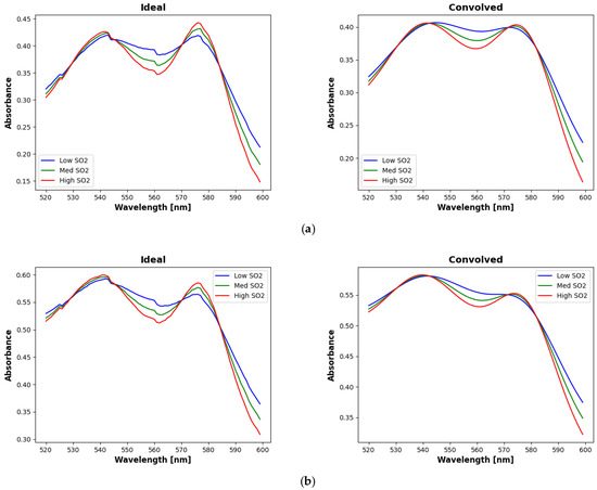
Figure 5.
Simulated absorption spectra for the ideal (left) and convolved (right) cases for (a) low melanin (<0.10) and (b) high melanin (>0.30) concentrations. Each plot shows example spectra for low (<0.60, blue), medium (0.60–0.80, green), and high (>0.80, red) SO2 values. Note that the separations between the curves near the higher wavelength lobe is greatly diminished for the convolved case relative to the ideal case.
Table 3.
Example wavelength selections.
Figure 5 shows examples of simulated spectra for low (<0.10), medium (0.10–0.30), and high (>0.30) SO2 values for both the ideal and the convolved cases. The spectra in Figure 5a represent skin with low melanin fractions (<0.10) and those in Figure 5b represent skin with high melanin fractions (>0.30). For both melanin fractions, there is a noticeable separation between the curves near the higher wavelength lobe for the ideal case. However, this separation is greatly diminished for the convolved case. Thus, the ability to distinguish between different SO2 values using wavelengths in this region is similarly diminished. Interestingly, wavelength selection does favor wavelengths near the lower wavelength lobe even though there is little separation between the curves in any of the plots of Figure 5. The selection of wavelengths in this region is likely needed more for slope estimation (third term in Equations (1) and (2)) than for SO2 estimation (second and fourth terms).
3.2. Validation Results
3.2.1. Monte Carlo Dataset
The mean prediction errors over the entire Monte Carlo validation dataset for the different numbers of selected wavelengths, k, are plotted in Figure 6, with the error bars representing one standard deviation. For both the ideal and the convolved cases, very low errors (<1%) are evident for all but the k = 3 case. Figure 7 shows these results separated by melanin fraction to represent light-skinned, moderately pigmented, and darkly pigmented adults. For all plots in both figures, we note the slight increase in prediction errors for the k = 81 case where all possible wavelengths are selected, suggesting that the inclusion of some wavelengths actually hurts the prediction accuracy due to as-yet unmodeled phenomena. This finding is consistent with other studies (e.g., [20]), which achieved higher estimation accuracy with fewer wavelengths than were available. The small, highly overlapping error bars for k > 3 indicate that there are no significant differences in the prediction errors for the different skin types, thus validating the proposed algorithm’s ability to not only accurately predict SO2, but to do so for all skin pigmentations.
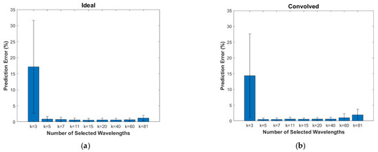
Figure 6.
Mean prediction error values for each number of selected wavelengths along with one-standard-deviation error bars for the (a) ideal case and the (b) convolved case. Values are computed from the entire Monte Carlo validation dataset.
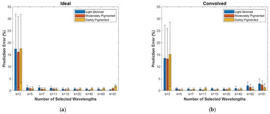
Figure 7.
Prediction errors for the Monte Carlo validation dataset separated by melanin fraction representing light-skinned (<0.10), moderately pigmented (0.10–0.30), and darkly pigmented (>0.30) adults. Mean values and one-standard-deviation error bars are given for (a) the ideal case and (b) the convolved case.
3.2.2. In Vivo Dataset
Since the true SO2 values for the in vivo dataset are unknown, the performance of the proposed algorithm was validated by its ability to yield differences in the SO2 predictions for the at-rest and the occlusion states that are statistically significant. Figure 8 shows the resulting mean-predicted SO2 values and one-standard-deviation error bars for these two states over all numbers of selected wavelengths. For all but the k = 3 experiment in the ideal case, the separation between the mean values for the at-rest and occlusion states is statistically significant, as determined via a two-tailed independent sample t-test (MATLAB’s ttest2 function) with a confidence level of 95%. However, there is noticeable fluctuation in the mean values for k < 20.
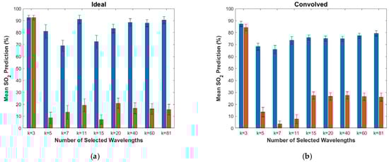
Figure 8.
Mean prediction values and one-standard-deviation error bars for the in vivo dataset for the different numbers of selected wavelengths. Values for the subjects in the at-rest state are shown in blue and for the occlusion state in red. Results are given for (a) the ideal case and (b) the convolved case.
Table 4 lists the time-averaged and student-averaged SO2 estimates for the at-rest and occlusion states, for both the ideal and the convolved cases, and compares these values with values from the recent literature. The SO2 estimates from this study are thus consistent with those of other studies for both the at-rest and occlusion conditions. However, we do note that there is considerable discrepancy between the ideal and convolved cases, with the convolved case yielding consistently lower at-rest SO2 values and higher occluded SO2 values. This discrepancy between the two cases is inconsistent with the findings with the Monte Carlo dataset discussed in the previous section. Without additional physiological data such as the true SO2 values and epidermal thicknesses, it is not possible to determine the exact cause of this discrepancy.
Table 4.
Time-averaged and student-averaged mean and standard deviation of SO2 estimates for the at-rest and occlusion conditions in this study (top) compared with values from recent literature (bottom).
3.3. Stability Test Results
Figure 9 shows the absolute differences in the prediction error resulting from the test to determine the stability of the proposed algorithm with respect to small changes in the selected peak wavelengths. The k > 3 experiments for the ideal case are shown to be very stable to fluctuations in peak wavelengths, with most of the error differences much less than 1%. Similar results can be seen for the convolved case, although there is noticeably more variation for the k = 7 and k = 11 cases, with differences in error reaching ~3%. Furthermore, the mean error differences shift away from zero for the k = 40 and k = 60 cases, reflecting the increases in the prediction error from the Monte Carlo validation study results shown in Figure 6. Given the reduction in complexity and expense offered by the hypothetical device enabled by the proposed algorithm, this potential for modest additional error may be an attractive trade off.
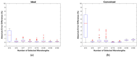
Figure 9.
Results of the stability testing for (a) the ideal case and (b) the convolved case. Boxplots are based on the differences in prediction error between the values for the adjusted wavelength sets and those for the exact wavelengths selected by the simulated annealing algorithm.
4. Conclusions
This study was designed to evaluate the potential for developing an inexpensive device for accurately estimating SO2, regardless of skin type, via narrowband spectroscopy with a small number of wavelengths. The proposed simulated annealing-based wavelength selection and EMLB-based SO2 estimation algorithm was found to yield SO2 estimates with low error (<1%), using as few as five wavelengths (524, 542, 553, 585, and 588 nm), in both simulated and in vivo validation datasets. Furthermore, these results were consistent across skin types of low, medium, and high melanin fractions. Additional testing proved that the proposed algorithm is robust to slight fluctuations in the peaks of the selected wavelengths, as might be experienced in a device constructed with cost-effective LEDs. Similarly, the algorithm proved to be robust to data convolution with a 15 nm FWHM Gaussian filter, another test conducted to model a more realistic device. However, the in vivo testing showed discrepancies between the estimated SO2 values for the ideal and convolved cases of ~10% on average. Future work will include in vivo testing with a larger group of subjects representing a more diverse set of skin types. Further algorithm development will account for varying peak wavelength uncertainties and LED bandwidths for the selected wavelengths and will include the expansion of the wavelength range of interest to include near-infrared.
Author Contributions
Conceptualization, G.B.; data curation, R.B. and A.H.; formal analysis, J.C. and A.H.; investigation, J.C. and R.B.; methodology, J.C., A.A. and A.H.; resources, A.H.; software, J.C.; supervision, A.A., F.V. and K.T.; visualization, J.C.; writing—original draft, J.C.; writing—review and editing, A.A. and A.H. All authors have read and agreed to the published version of the manuscript.
Funding
This research received no external funding.
Institutional Review Board Statement
The study was conducted according to the guidelines of the Declaration of Helsinki, and approved by the edical Executive Committee in the clinical center of the Universiti Tun Hussein Onn Malaysia (UTHM).
Informed Consent Statement
Informed consent was obtained from all subjects involved in the study.
Data Availability Statement
Not applicable.
Conflicts of Interest
The authors declare no conflict of interest.
References
- Saeedi, P.; Petersohn, I.; Salpea, P.; Malanda, B.; Karuranga, S.; Unwin, N.; Colagiuri, S.; Guariguata, L.; Motala, A.A.; Ogurtsova, K.; et al. Global and regional diabetes prevalence estimates for 2019 and projections for 2030 and 2045: Results from the International Diabetes Federation Diabetes Atlas, 9th edition. Diabetes Res. Clin. Pract. 2019, 157, 107843. [Google Scholar] [CrossRef] [PubMed]
- International Diabetes Foundation, IDF Diabetes Atlas|Tenth Edition. Available online: https://diabetesatlas.org/ (accessed on 18 June 2022).
- Oliver, T.I.; Mutluoglu, M. Diabetic Foot Ulcer. In StatPearls; StatPearls Publishing: Treasure Island, FL, USA, 2022. Available online: http://www.ncbi.nlm.nih.gov/books/NBK537328/ (accessed on 18 June 2022).
- Armstrong, D.G.; Boulton, A.J.M.; Bus, S.A. Diabetic Foot Ulcers and Their Recurrence. N. Engl. J. Med. 2017, 376, 2367–2375. [Google Scholar] [CrossRef] [PubMed]
- Raghav, A.; Khan, Z.A.; Labala, R.K.; Ahmad, J.; Noor, S.; Mishra, B.K. Financial burden of diabetic foot ulcers to world: A progressive topic to discuss always. Ther. Adv. Endocrinol. Metab. 2018, 9, 29–31. [Google Scholar] [CrossRef] [PubMed]
- Jodheea-Jutton, A.; Hindocha, S.; Bhaw-Luximon, A. Health economics of diabetic foot ulcer and recent trends to accelerate treatment. Foot 2022, 101909. [Google Scholar] [CrossRef]
- Diabetes and African Americans—The Office of Minority Health. 2021. Available online: https://minorityhealth.hhs.gov/omh/browse.aspx?lvl=4&lvlid=18 (accessed on 18 June 2021).
- Prevalence of Diagnosed Diabetes|Diabetes|CDC. 2022. Available online: https://www.cdc.gov/diabetes/data/statistics-report/diagnosed-diabetes.html (accessed on 18 June 2022).
- Tran, P.; Tran, L.; Tran, L. Impact of rurality on diabetes screening in the US. BMC Public Health 2019, 19, 1190. [Google Scholar] [CrossRef]
- The Burden of Diabetes in Rural America: Rural Health Research Project. Available online: https://www.ruralhealthresearch.org/projects/100002380 (accessed on 18 June 2022).
- Sharma, R.; Sharma, S.K.; Mudgal, S.K.; Jelly, P.; Thakur, K. Efficacy of hyperbaric oxygen therapy for diabetic foot ulcer, a systematic review and meta-analysis of controlled clinical trials. Sci. Rep. 2021, 11, 2189. [Google Scholar] [CrossRef]
- Dietrich, M.; Marx, S.; von der Forst, M.; Bruckner, T.; Schmitt, F.C.F.; Fiedler, M.O.; Nickel, F.; Studier-Fischer, A.; Müller-Stich, B.P.; Hackert, T.; et al. Hyperspectral imaging for perioperative monitoring of microcirculatory tissue oxygenation and tissue water content in pancreatic surgery—An observational clinical pilot study. Perioper. Med. 2021, 10, 42. [Google Scholar] [CrossRef]
- Oshina, I.; Spigulis, J. Beer–Lambert law for optical tissue diagnostics: Current state of the art and the main limitations. J. Biomed. Opt. 2021, 26, 100901. [Google Scholar] [CrossRef]
- Vyas, S.; Banerjee, A.; Burlina, P. Estimating physiological skin parameters from hyperspectral signatures. J. Biomed. Opt. 2013, 18, 057008. [Google Scholar] [CrossRef]
- Yudovsky, D.; Pilon, L. Retrieving skin properties from in vivo spectral reflectance measurements. J. Biophotonics 2011, 4, 305–314. [Google Scholar] [CrossRef]
- Saiko, G.; Lombardi, P.; Au, Y.; Queen, D.; Armstrong, D.; Harding, K. Hyperspectral imaging in wound care: A systematic review. Int. Wound J. 2020, 17, 1840–1856. [Google Scholar] [CrossRef]
- Lee, C.J.; Walters, E.; Kennedy, C.J.; Beitollahi, A.; Evans, K.K.; Attinger, C.E.; Kim, P.J. Quantitative Results of Perfusion Utilising Hyperspectral Imaging on Non-diabetics and Diabetics: A Pilot Study. Int. Wound J. 2020, 17, 1809–1816. [Google Scholar] [CrossRef] [PubMed]
- Vasefi, F.; MacKinnon, N.; Saager, R.B.; Durkin, A.J.; Chave, R.; Lindsley, E.H.; Farkas, D.L. Polarization-Sensitive Hyperspectral Imaging in vivo: A Multimode Dermoscope for Skin Analysis. Sci. Rep. 2014, 4, 4924. [Google Scholar] [CrossRef] [PubMed]
- Saager, R.B.; Sharif, A.; Kelly, K.M.; Durkin, A.J. In vivo isolation of the effects of melanin from underlying hemodynamics across skin types using spatial frequency domain spectroscopy. J. Biomed. Opt. 2016, 21, 057001. [Google Scholar] [CrossRef] [PubMed]
- Ayala, L.; Isensee, F.; Wirkert, S.J.; Vemuri, A.S.; Maier-Hein, K.H.; Fei, B.; Maier-Hein, L. Band selection for oxygenation estimation with multispectral/hyperspectral imaging. Biomed. Opt. Express 2022, 13, 1224. [Google Scholar] [CrossRef]
- Marois, M.; Jacques, S.L.; Paulsen, K.D. Optimal wavelength selection for optical spectroscopy of hemoglobin and water within a simulated light-scattering tissue. J. Biomed. Opt. 2018, 23, 071202. [Google Scholar] [CrossRef]
- Huong, A.; Ngu, X. The application of extended modified Lambert Beer model for measurement of blood carboxyhemoglobin and oxyhemoglobin saturation. J. Innov. Opt. Health Sci. 2014, 7, 1450026. [Google Scholar] [CrossRef]
- Philimon, S.P.; Huong, A.K.C.; Ngu, X.T.I. Tissue Oxygen Level in Acute and Chronic Wound: A Comparison Study. J. Teknol. 2020, 82, 131–140. [Google Scholar] [CrossRef]
- Twersky, V. Absorption and Multiple Scattering by Biological Suspensions. J. Opt. Soc. Am. 1970, 60, 1084–1093. [Google Scholar] [CrossRef]
- Huong, A.K.C.; Philimon, S.P.; Ngu, X.T.I. Noninvasive Monitoring of Temporal Variation in Transcutaneous Oxygen Saturation for Clinical Assessment of Skin Microcirculatory Activity. In Proceedings of the International Conference for Innovation in Biomedical Engineering and Life Sciences: ICIBEL2015, Putrajaya, Malaysia, 6–8 December 2015; pp. 248–251. [Google Scholar] [CrossRef]
- Huong, A.; Tay, K.G.; Ngu, X. Towards Skin Tissue Oxygen Monitoring: An Investigation of Optimal Visible Spectral Range and Minimal Spectral Resolution. Univers. J. Electr. Electron. Eng. 2019, 6, 49–54. [Google Scholar] [CrossRef]
- Wang, L.; Jacques, S.L.; Zheng, L. MCML—Monte Carlo modeling of light transport in multi-layered tissues. Comput. Methods Programs Biomed. 1995, 47, 131–146. [Google Scholar] [CrossRef]
- Tsumura, N.; Kawabuchi, M.; Haneishi, H.; Miyake, Y. Mapping Pigmentation in Human Skin by Multi-Visible-Spectral Imaging by Inverse Optical Scattering Technique. In Proceedings of the Eighth Color Imaging Conference: Color Science, Systems and Applications, Scottsdale, AZ, USA, 7–10 November 2000; pp. 81–84. [Google Scholar]
- Alerstam, E.; Svensson, T.; Andersson-Engels, S. Parallel computing with graphics processing units for high-speed Monte Carlo simulation of photon migration. J. Biomed. Opt. 2008, 13, 060504. [Google Scholar] [CrossRef] [PubMed]
- Jacques, S.L. Skin Optics Summary. 1998. Available online: https://omlc.org/news/jan98/skinoptics.html (accessed on 1 January 2022).
- Scipy.Ndimage.Gaussian_Filter1d—SciPy v1.9.0 Manual. Available online: https://docs.scipy.org/doc/scipy/reference/generated/scipy.ndimage.gaussian_filter1d.html (accessed on 8 August 2022).
- Belay, A. Measurement of integrated absorption cross-section, oscillator strength and number density of caffeine in coffee beans by integrated absorption coefficient technique. Food Chem. 2010, 121, 585–590. [Google Scholar] [CrossRef]
- LUXEON Z Color Line. Lumileds. Available online: https://lumileds.com/products/color-leds/luxeon-z-colors/ (accessed on 23 June 2022).
- Unmounted LEDs. Available online: https://www.thorlabs.com/newgrouppage9.cfm?objectgroup_id=2814#4475 (accessed on 23 June 2022).
- Visible LEDs|Ocean Insight. Available online: https://www.oceaninsight.com/products/light-sources/leds/vis-leds/ (accessed on 23 June 2022).
- LP T655-Q1R2-25 ams OSRAM|Mouser. Mouser Electronics. Available online: https://www.mouser.com/ProductDetail/N-A (accessed on 23 June 2022).
- Binzoni, T.; Vogel, A.; Gandjbakhche, A.H.; Marchesini, R. Detection limits of multi-spectral optical imaging under the skin surface. Phys. Med. Biol. 2008, 53, 617–636. [Google Scholar] [CrossRef] [PubMed]
- Meglinski, I.; Matcher, S. Computer simulation of the skin reflectance spectra. Comput. Methods Programs Biomed. 2003, 70, 179–186. [Google Scholar] [CrossRef]
- Meglinski, I.V.; Matcher, S.J. Quantitative assessment of skin layers absorption and skin reflectance spectra simulation in the visible and near-infrared spectral regions. Physiol. Meas. 2002, 23, 741–753. [Google Scholar] [CrossRef]
- Prahl, S.A. Optical Absorption of Hemoglobin. Available online: https://omlc.org/spectra/hemoglobin/ (accessed on 11 June 2022).
- Van Staveren, H.J.; Moes, C.J.M.; Van Marie, J.; Prahl, S.A.; Van Gemert, M.J.C. Light scattering in lntralipid-10% in the wavelength range of 400–1100 nm. Appl. Opt. 1991, 30, 4507–4514. [Google Scholar] [CrossRef]
- Bashkatov, A.N.; Genina, E.A.; Kochubey, V.I.; Tuchin, V.V. Optical properties of human skin, subcutaneous and mucous tissues in the wavelength range from 400 to 2000 nm. J. Phys. D Appl. Phys. 2005, 38, 2543–2555. [Google Scholar] [CrossRef]
- Nishidate, I.; Aizu, Y.; Mishina, H. Estimation of melanin and hemoglobin in skin tissue using multiple regression analysis aided by Monte Carlo simulation. J. Biomed. Opt. 2004, 9, 700–710. [Google Scholar] [CrossRef]
- Bertsimas, D.; Tsitsiklis, J. Simulated Annealing. Stat. Sci. 1993, 8, 20–69. [Google Scholar] [CrossRef]
- Caspary, L.; Thum, J.; Creutzig, A.; Lübbers, D.; Alexander, K. Quantitative Reflection Spectrophotometry: Spatial and Temporal Variation of Hb Oxygenation in Human Skin. Int. J. Microcirc. 1995, 15, 131–136. [Google Scholar] [CrossRef] [PubMed]
- Zhang, R.; Verkruysse, W.; Choi, B.; Viator, J.A.; Jung, B.; Svaasand, L.O.; Aguilar, G.; Nelson, J.S. Determination of human skin optical properties from spectrophotometric measurements based on optimization by genetic algorithms. J. Biomed. Opt. 2005, 10, 024030–02403011. [Google Scholar] [CrossRef]
- Kobayashi, M.; Ito, Y.; Sakauchi, N.; Oda, I.; Konishi, I.; Tsunazawa, Y. Analysis of nonlinear relation for skin hemoglobin imaging. Opt. Express 2001, 9, 802–812. [Google Scholar] [CrossRef] [PubMed]
- Thorn, C.E.; Matcher, S.J.; Meglinski, I.V.; Shore, A. Is mean blood saturation a useful marker of tissue oxygenation? Am. J. Physiol. Circ. Physiol. 2009, 296, H1289–H1295. [Google Scholar] [CrossRef] [PubMed]
- Kyle, B.; Litton, E.; Ho, K.M. Effect of hyperoxia and vascular occlusion on tissue oxygenation measured by near infra-red spectroscopy (InSpectra™): A volunteer study. Anaesthesia 2012, 67, 1237–1241. [Google Scholar] [CrossRef] [PubMed]
- Bezemer, R.; Lima, A.; Myers, D.; Klijn, E.; Heger, M.; Goedhart, P.T.; Bakker, J.; Ince, C. Assessment of tissue oxygen saturation during a vascular occlusion test using near-infrared spectroscopy: The role of probe spacing and measurement site studied in healthy volunteers. Crit. Care 2009, 13, S4. [Google Scholar] [CrossRef] [PubMed]
- Vogel, A.; Chernomordik, V.V.; Riley, J.D.; Hassan, M.; Amyot, F.; Dasgeb, B.; Demos, S.G.; Pursley, R.; Little, R.F.; Yarchoan, R.; et al. Using noninvasive multispectral imaging to quantitatively assess tissue vasculature. J. Biomed. Opt. 2007, 12, 051604. [Google Scholar] [CrossRef][Green Version]
- Ferrari, M.; Binzoni, T.; Quaresima, V. Oxidative metabolism in muscle. Philos. Trans. R. Soc. Lond. B Biol. Sci. 1997, 352, 677–683. [Google Scholar] [CrossRef]
Publisher’s Note: MDPI stays neutral with regard to jurisdictional claims in published maps and institutional affiliations. |
© 2022 by the authors. Licensee MDPI, Basel, Switzerland. This article is an open access article distributed under the terms and conditions of the Creative Commons Attribution (CC BY) license (https://creativecommons.org/licenses/by/4.0/).