Aerodynamic Benefits by Optimizing Cycling Posture

Abstract

An approach to aerodynamically optimizing cycling posture and reducing drag in an Ironman (IM) event was elaborated. Therefore, four commonly used positions in cycling were investigated and simulated for a flow velocity of 10 m/s and yaw angles of 0–20° using OpenFoam-based Nabla Flow CFD simulation software software. A cyclist was scanned using an IPhone 12, and a special-purpose meshing software BLENDER was used. Significant differences were observed by changing and optimizing the cyclist’s posture. Aerodynamic drag coefficient (CdA) varies by more than a factor of 2, ranging from 0.214 to 0.450. Within a position, the CdA tends to increase slightly at yaw angles of 5–10° and decrease at higher yaw angles compared to a straight head wind, except for the time trial (TT) position. The results were applied to the IM Hawaii bike course (180 km), estimating a constant power output of 300 W. Including the wind distributions, two different bike split models for performance prediction were applied. Significant time saving of roughly 1 h was found. Finally, a machine learning approach to deduce 3D triangulation for specific body shapes from 2D pictures was tested.

1. Introduction

Aerodynamic drag is crucial in cycling. It is one of the most limiting factors and therefore, bears the greatest potential for improvement [1,2]. For many professional cyclists and triathletes, it is about saving energy as much as possible. Those savings can be achieved by riding in a group or optimizing the cycling posture. In a team time trial event or in a small group of up to nine cyclists riding at the same speed, savings of up to 50–60% can be observed, depending on the cyclist’s position and distance from the teammate in front [3]. In large pelotons, groups of 100 plus riders, the effect multiplies and becomes even more significant. Savings and drag reductions of 5% for an isolated cyclist at the back of the peloton can be found. These cyclists hardly have to pedal at common racing speeds of 15 m/s (54 km/h). Not only does the cyclist at the back of the peloton experience a drag reduction, but the leading cyclist does, due to the upstream flow disturbance caused by the riders behind him/her [4].

Knowledge about aerodynamic drag is not only used in professional road cycling, it also in related sports such as the triathlon, especially in long distance/Ironman (IM) events. An IM consists of a 3.8 km swim, followed by a 180 km bike ride and a closing 42.2 km marathon run. In this case, saving energy for the upcoming run is decisive. Despite the fact that drafting, i.e., direct riding behind one and another, is strictly forbidden in these events, refs. [3,5] indicated the benefits of riding 10 m behind a competitor, within the permitted range.

At racing speeds of 15 m/s, the aerodynamic drag makes for up about 90% of the total resistance [6,7,8]. This major part is split into two components: 70% is due to the cyclist and 30% is due to the bike [9]. Since the majority of the aerodynamic drag of the athlete is caused by the athlete’s body itself, different cycling postures will have significant effects on the speed he/she is traveling at [8,10,11]. Thus, even relatively small changes in posture, such as changing arm position, can result in noteworthy savings [12].

Our main purpose was to quantify the impacts of four positions and present them by showing the resulting time savings on the 180 km IM World Championship course in Hawaii, considering realistic yaw angles of 0–20°. The elevation profile and weather data of the IM Hawaii bike course are well known, so the course is highly suitable for this work. For this purpose, a 3D scan of a professional male athlete was performed, and different cycling postures were observed. As a low cost approach and novelty presented in this work, the scan was performed by using a commercially available iPhone 12 Pro with a LIDAR Scanner. The scan was then post-processed using the open-source Software Blender. Flow simulations were run in Nabla Flow’s in-house simulation software AeroCloud, an OpenFoam-based CFD tool.

Comparable investigations have been conducted by [13,14,15] to name a few. Crouch et al. [15] have the most recent excellent review on the importance of bluff-body aerodynamics for elite level cycling, as they called it.

2. Methods

Four commonly used positions in cycling were investigated and simulated for a flow velocity of 10 m/s and yaw angles of 0–20°. For the mesh preparation, a 3D scan was performed with an iPhone12 Pro using an in-built Lidar scanner.

2.1. Determination of a Realistic 3D Cyclist Geometry

A 3D scan approach was used to obtain a sufficiently detailed geometry. Due to high cost and low availability of professional 3D scanners; however, a low cost approach using a state-of-the-art iPhone 12 Pro with a Lidar Scanner was performed in this study. To be more specific, the following scan parameters were chosen, which still needed a calm hand during the scanning process. A typical attempt took approximately five minutes of scan time.

• Name: 3D Scanner App.
• Source: https://apps.apple.com/us/app/3d-scanner-app/id1419913995 (accessed on 22 August 2021).
• Masking: Person mode.
• Resolution: 7 mm—(possible: 5 mm–20 mm).
• Scan Range: 2.0 m (possible: 0.3 m–5 m).
• Resolution: High.
• Confidence: High.
• output format: STL.

The initial mesh was processed using Blender 2.9 (open-source), including cleaning from unattached voxels, filling holes, smoothing and meshing the full computational volume. As a result, a 3D structure was detected and reconstructed.

The scanned cyclist measuring 1.96 m and weighing 82 kg is a professional triathlete. He was scanned on his road bike wearing a race trisuit, an aero helmet, bike socks and road bike shoes, which directly attach to the bike (the used road bike was a Cannondale Caad 10; the trisuit is by swim brand Arena; the Helmet was provided by Scott and the shoes by Fizik). The rear wheel was taken off and the bike was mounted on a Tacx Neo 2T direct drive home trainer, which replaced the shifting on the rear wheel and ensured stable positioning on the ground.

The originally scanned position is a commonly used position amongst cyclists during training rides where the cyclist is sitting comfortably with straight arms and hands on the hoods (HH). During the scan, the legs and feet were positioned statically with horizontal crank. Static leg positioning; however, would not have affected the simulation results compared to dynamic pedaling [16].

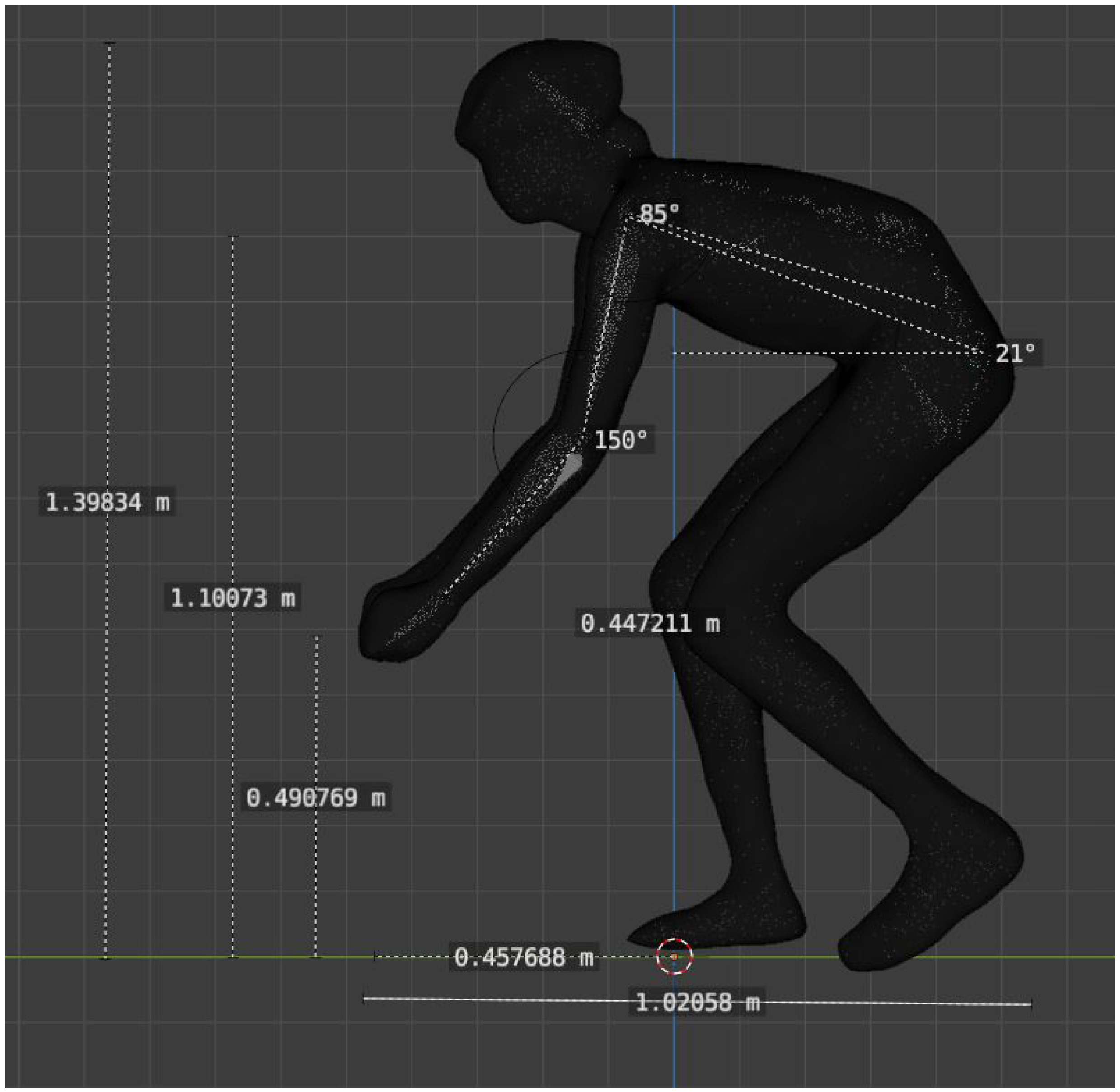
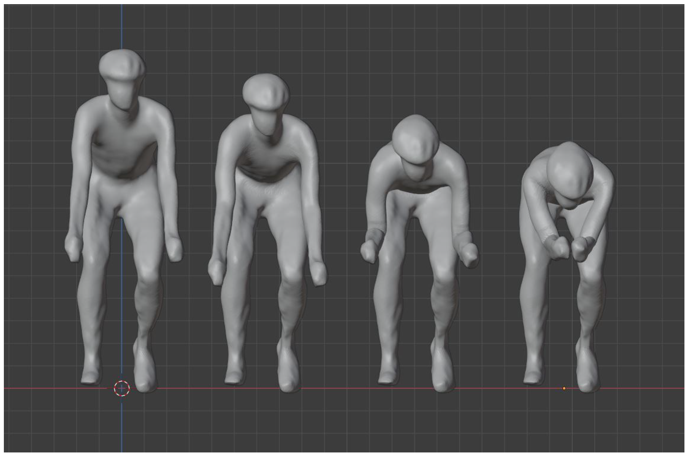
The different positions analyzed are presented in Figure 1. The dimensions and bio-mechanical angles are shown for the HD position in Figure 2. All biomechanical parameters used for modifying the position are presented in

Table 1. Cyclist’s dimensions and geometry.

Dimensions and Geometry	HH	HD	DB	TT
Cyclist’s height [m]	1.50	1.40	1.22	1.10
Cyclist’s length [m]	1.02	1.02	1.02	1.17
Cyclist’s height to shoulders [m]	1.21	1.10	1.00	0.94
Exaggeration [m]	0.16	0.26	0.16	0.16
Upper arm length [m]	0.32	0.32	0.32	0.32
Lower arm length [m]	0.32	0.32	0.32	0.32
Shoulder width [m]	0.44	0.44	0.44	0.44
Arm width [m]	0.44	0.44	0.44	0.15
Hands above feet [m]	0.59	0.49	0.59	0.59
Hip angle [°]	37	21	13	4
Shoulder angle [°]	95	85	76	108
Arm angle [°]	163	150	97	112

.

• HH: Scanned position. Rider is sitting comfortably with straight arms and hands on the hoods.
• HD: Modeled position. Rider is sitting a little bit more aggressively now; arms are slightly bent and hands are in the drops.
• DB: Modeled position. Rider is sitting a lot more aggressively now. Body is dropped; arms are fully bent and hands are locked horizontally on the hoods.
• TT: Modeled position, rider is sitting a lot more aggressively now. Body is dropped; arms are fully bent and brought together only lying at the middle of the handlebars. Stability in reality would be guaranteed by arm cups on the handlebar.

2.2. Post-Processing of the 3D Scan, Meshing, Validation

For the scanned HH position, a STL-file was generated which then was imported into the open-source graphics software Blender 2.9. Postprocessing work and meshing the body structure were performed in Blender as well. It is known from a comparable case [17] that an accuracy of 2% (in terms of cdA) may be reached after refinement from a volume mesh containing 2 M cells to a 55 M mesh. Our mesh-dependency study is summarized in

Table 2. Data used in mesh dependency study. nVC: number of volume cells (tets), nSC: number of surface cells (triangles) of cyclist’s body.

	nVC (M)	nSC (k)	1/nVC	Drag (N)	CdA	Dev. (%)
coarse	0.24	4.167	2.7	2.24	0.036	65.0
medium	0.67	1.493	69.0	6.14	0.100	3.2
medium	0.71	1.416	69.5	6.61	0.108	4.3
fine	2.55	0.392	279	6.49	0.106	2.4

. Deviation was extrapolated form a mutual exact value by a Richardson extrapolation. Here drag was fitted as a function of inverse mesh-size (1/ms) by a quadratic polynomial, and then the limit $ms\to \infty$ was taken. As a result, accuracy in CdA of a few percentage points was reached with medium-sized meshes according Table 2.

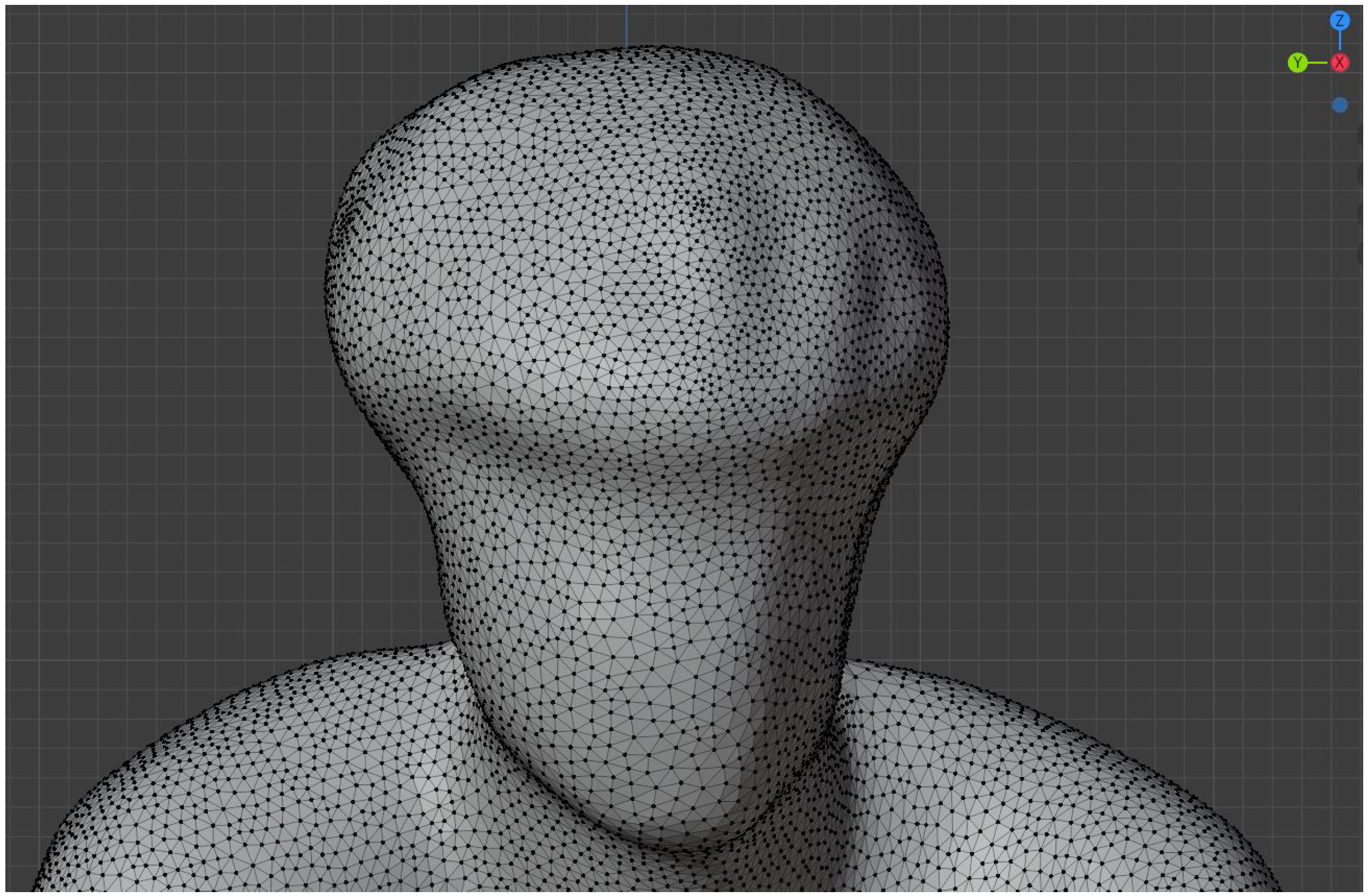
The finally used surface mesh contained 78,490 vertices and 156,976 triangles with a side length below 9 mm, and it fits well into the category of medium-sized mesh described by [17].

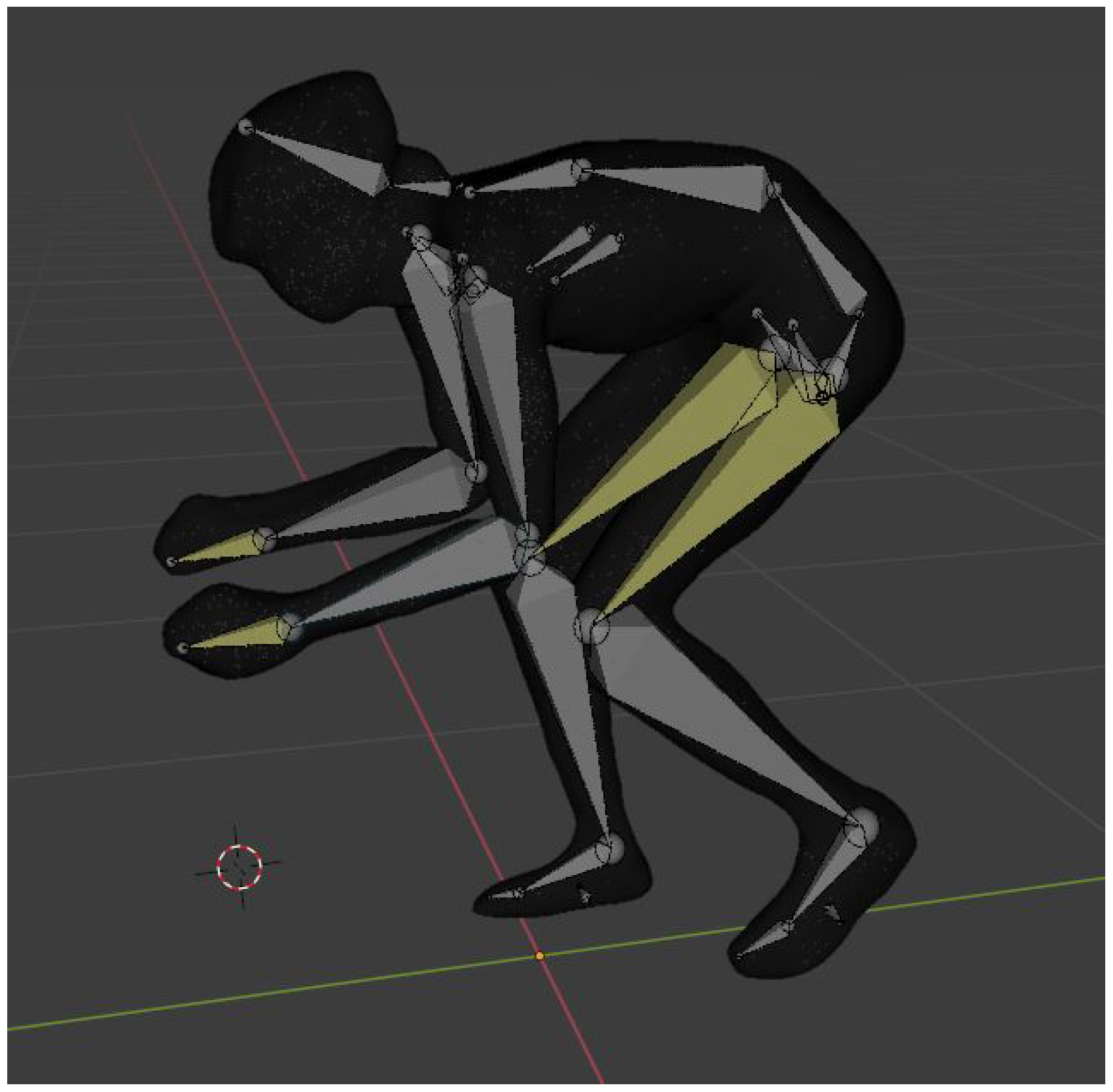
The meshed cyclist’s head is shown in Figure 3. After preparing the original position, a so-called metarig was implemented and connected to the 3D geometry. A metarig is a skeleton of the human body reduced to its essential bones and moving joints. DB position is shown in Figure 4. As mentioned above, some bone constraints were set for arms and legs to ensure accurate changes in the target positions. For the simulation using Nabla Flow, all models were rotated around the z-axis to account for yaw angles ranging from 5° to 20° in steps of 5°.

2.3. Using Machine Learning to Simplify Mesh Generation

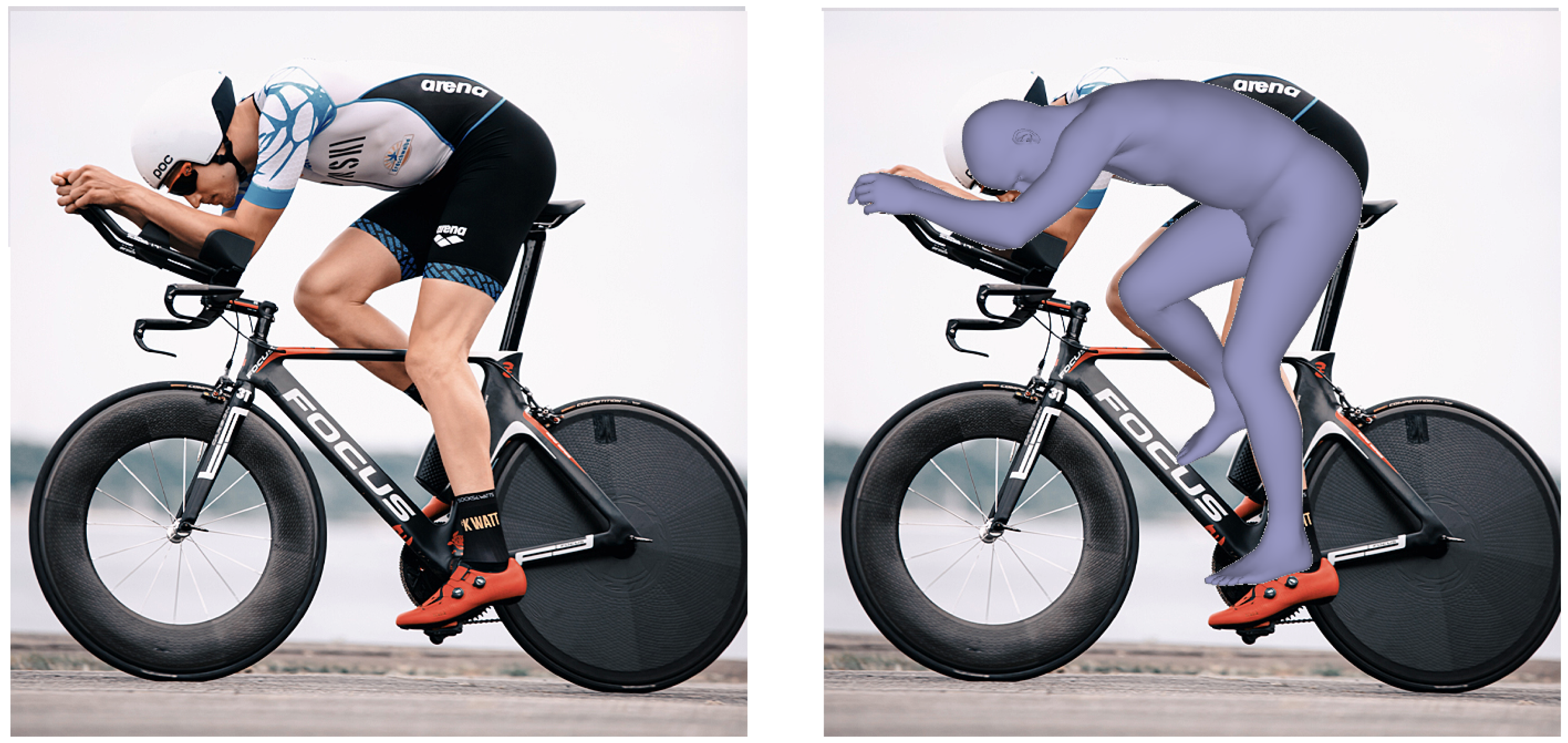
The 3D scan presented in this paper was created using an iPhone, making it more accessible than expensive commercial 3D scanners. Although the quality of the iPhone scan required sufficient post-processing time before a valid mesh was prepared, the overall result was promising. To further simplify the process of time-consuming and costly geometry acquisition via 3D scanning techniques, a machine learning method for deriving 3D triangulations for specific body shapes from pure 2D pictures was tested. The machine learning algorithm ExPose [18], open-source code for converting 2D images into 3D STL-files, was used, but it was found that it needs to be trained more specifically for typical body shapes and sports movements. Although its accuracy was considered to be currently not satisfactory, it already shows promising results; see Figure 5.

3. Results for Determining Aerodynamic Drag

3.1. Flow Simulation

Simulations were run with Nabla Flow in-house CFD software AeroCloud. A test simulation for the regular HH position at 0° was performed and validated with real power output data from training rides and showed satisfactory accuracy.

The simulation showed a CdA value of 0.294 with a projected frontal area of 0.468 m². The obtained CdA value is comparable to other studies, e.g., [10]. The corresponding drag force $F_d$ is 18 N, which leads to a power output of 180 W at a flow velocity of 10 m/s. Taking the bike into account as well, a total power output in a range of $240\pm 20$ W is needed to maintain constant speed (as previously stated, 70–80% of the drag is caused by the cyclist; the rest is due to the bike, mechanical losses within the drive-train and friction between wheels and road [9]). These results were compared to real data samples of the cyclist’s training history, cycling at 10 m/s ± 0.14 m/s. A total of 460 km of training rides were analyzed, thereof 120 km cycling outside using an Assioma Favero Uno pedal system and 340 km indoors on a Tacx Neo 2T, both considered with an accuracy of $\pm 1\%$. The outdoor segments had a length of 5 to 10 km. The indoor samples were longer, varying from 5 to 75 km.

3.2. Main Findings from Flow Simulation

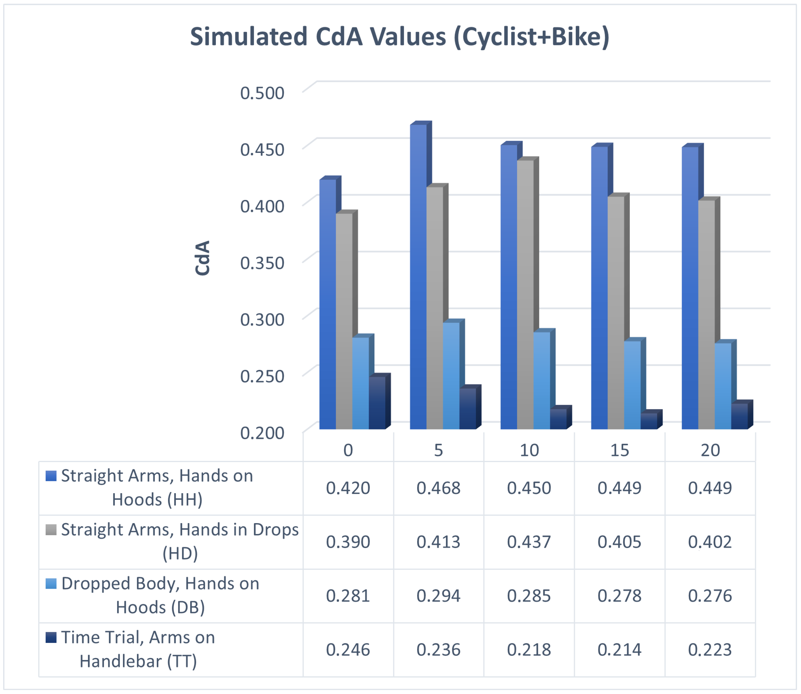
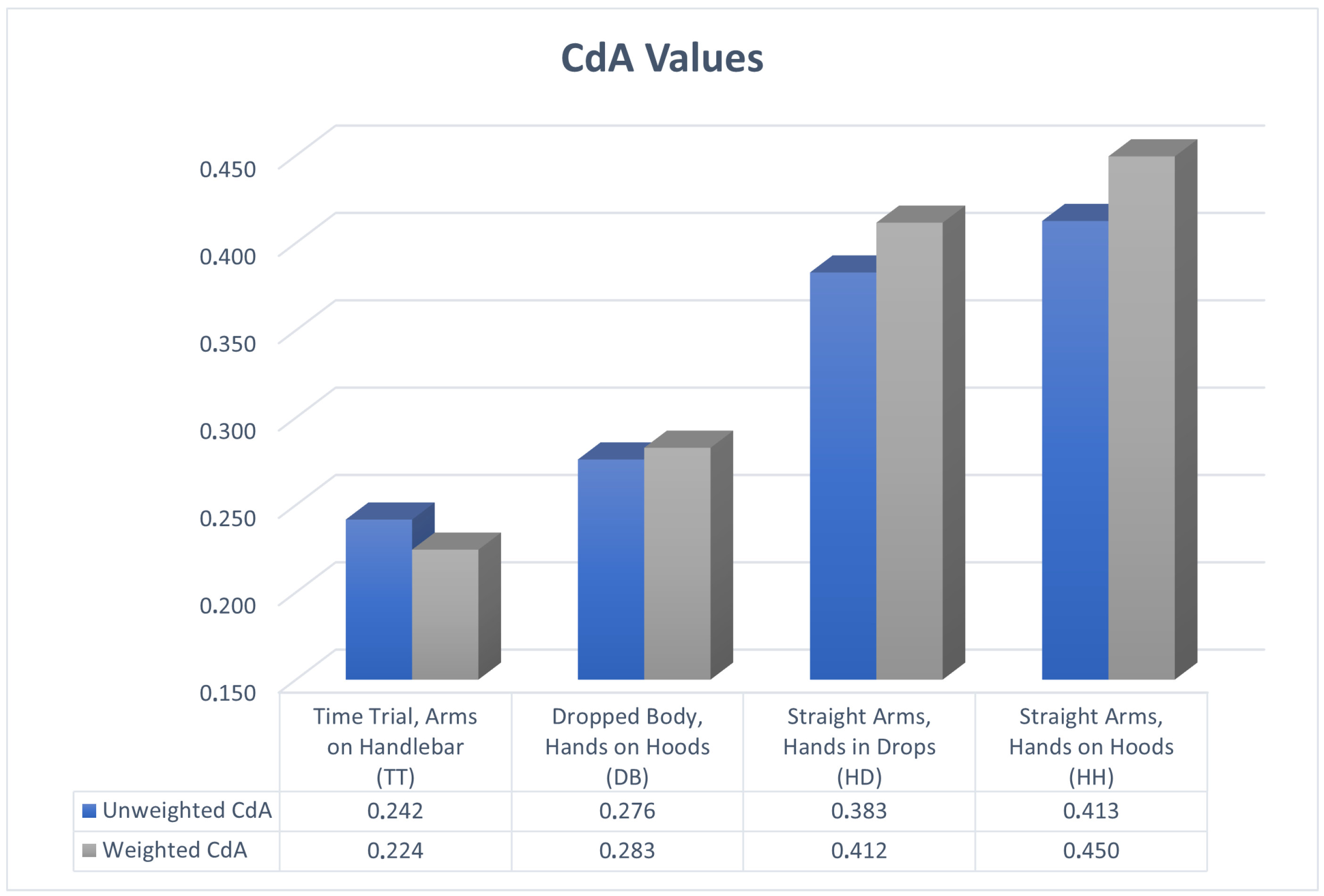
The flow velocity of 10 m/s was used to fit for typical Reynolds numbers. Values for the cyclist and the bike are presented in Figure 6. The impacts of the four different cycling positions are very clear. While the initial HH position shows CdA values in the range of 0.42 and 0.47, and therefore, the worst values, the TT position shows the best performance with CdA values between 0.22 and 0.24 Moreover, the two more comfortable positions (HH and HD) seem to be significantly more vulnerable to crosswinds, especially at 5–10° wind yaw: see the CdA that is higher by 0.034 (HH) or 0.033 (HD). The more aggressive positions (DB and TT) show more stability in crosswinds. They even tend to decrease at higher wind yaw. The TT position is even more favorable to crosswind then the DB position, with a CdA that is lower by 0.022–0.150. The yaw-dependence of CdA-values, shown Figure 6 reveals that all positions except (TT) show some increase at non-zero values, but only TT’s CdA seems to decrease with higher yaw angles. This is somewhat counter-intuitive, as the projected area at least increases by simply looking at the geometry.

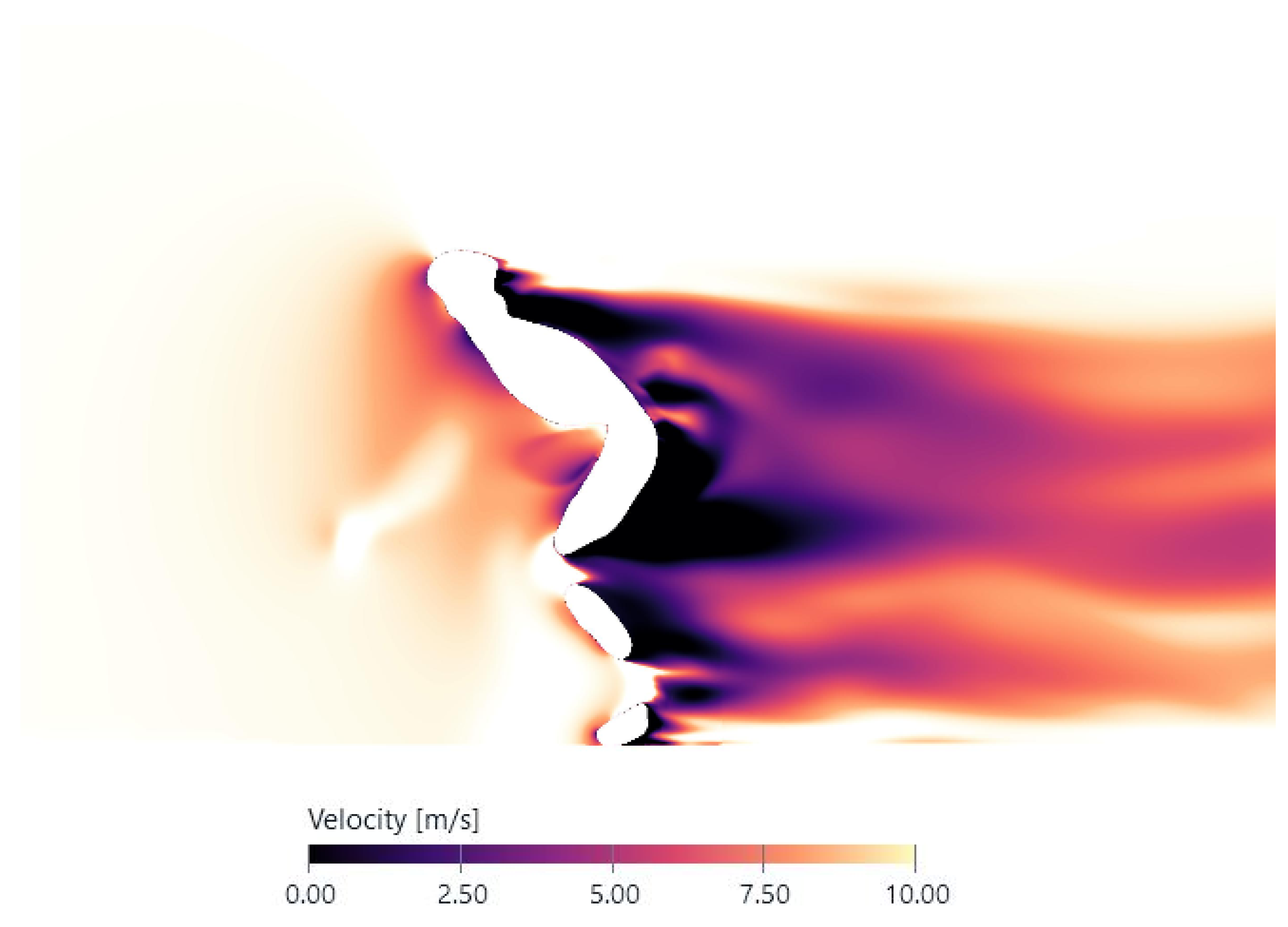
The corresponding flow wake along the models, sliced for the flow velocity in y-direction, is presented in Figure 7, showing large areas of dead air. Those areas of low speed often combine with regions of under-pressure, causing large areas of pressure-drag. Compared to the flow wake of the HH position at 20°, however, the flow wake in the TT position is a lot smoother and less disturbed.

Figure 7 gives an impression of the near-wake structure. Black areas indicate negative velocities, zones of re-circulating flow. It is well known that avoidance of these regions gives rise to reduced drag.

Additionally, to the CdA values, the resulting power output at 10 m/s was calculated. (In the example, the temperature T was set to 15.3 °C and aerodynamical drag was split into parts of 70% (cyclist) and 30% (bike).) While the HH position requires $190\pm 10$ W for the cyclist or $270\pm 15$ W including the bike for a speed of 10 m/s, the TT position only requires 50% of that power for the same speed, so $97\pm 8$ W for the cyclist and $140\pm 12$ W for the entire system. In the HD position, savings of around 8% compared to the HH positions can be observed. For the DB position, even higher savings of around 37% can be found, which makes the DB position the second fastest after the TT position. The calculated power output indicates very well the impact of cycling posture and the considerable energy savings that can be achieved.

These investigations make clear that the favorable TT position requires only half of the power compared to the HH position. Results from flow simulation may be summarized as follows:

• The lowest CdA value of 0.150 was reached for the TT position at 20°.
• The highest CdA value of 0.328 was reached for the HH position at 5°.
• Overall, the TT position showed the best performance.
• The TT position requires only half of the power output for the same speed as the HH position.
• DB and TT positions show much more stable performance in crosswinds, decreasing the crosswind’s effect at higher wind yaw.

3.3. Comparison of CdA Values from Other Sources

A short note on findings of other researchers is presented here. References [14,15] give extensive discussions; in both cases, Table 2 should be considered as especially suited for comparison. Minimum values vary from 0.21 to 0.24, in good agreement with our (TT) value of 0.25. If one compares UP position-values from [14] 0.25 to 0.3 with our (HH) position-value (0.42), one recognizes a larger deviation. One reason is a somewhat larger projected area ($0.42\dots 0.56$) in comparison to ours (0.48 m${}^2$) Nevertheless, one has to bear in mind that the accuracy of drag estimation using a RANS solver is mainly limited by the accurate prediction of the turbulent separation of boundary layers. From the long-reaching experience of one of the authors (APS), the realistic uncertainty is 10% (with regard to $c_D$).

4. Application to Ironman Hawaii

A bike split model was developed for application to the IM World Championship course on Big Island, Hawaii.

4.1. The Bike Course

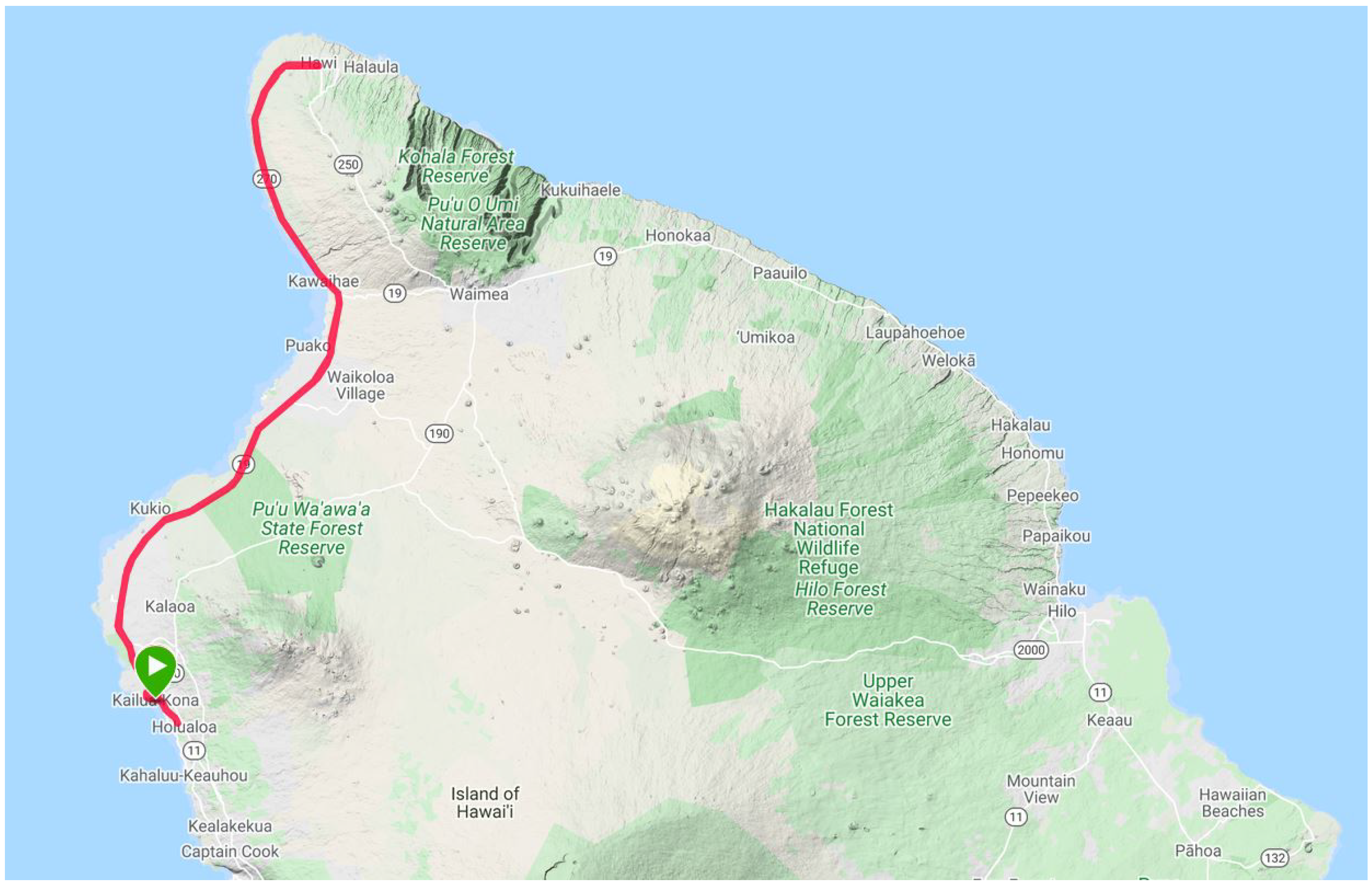
The IM Hawaii venue has been hosting the World Championships for more than 40 years. The hot and humid weather conditions of around 30 °C and even higher and the famous “ho’omumuku” crosswinds of up to 20 m/s on the bike make the race challenging for long distance athletes. The bike course has a length of 180 km and has been in place since 1981 without major changes [19]. Hence, course and wind data are well known and available in detail. The start and finish of the course is in Kailua-Kona directly on the pier. At first riders head south on Kuakini Highway for about 7.5 km, before turning back to Kailua-Kona and heading north all the way up to Hawi, the northernmost point of the island and the highest point on the course. After the turning point, the course leads back the same way on the Queen K’ Highway to Kailua-Kona, where the athletes compete in the final marathon as Figure 8.

The overall course has only a few turns where the athletes need to brake or accelerate, which is one of the reasons to use this course for the bike split model. Moreover, the elevation profile of the course, is relatively smooth, habing an overall ascent of 1238 m. Besides the short and steep uphill section on Palani Road in Kailua-Kona, it has a rolling hill profile with moderate inclines of up to 6%. The slope angle distribution was evaluated by Aerotune, Flensburg, Germany. As a result, 95.1% of the slope angles are represented within the interval of −2 to 4%, with the majority thereof (81.2%) being nearly completely flat.

4.2. Wind Data for IM Hawaii

Wind and weather conditions at IM Hawaii are well known and documented. The event takes place on the exact same weekend every year in October—there are no seasonal changes. Compared to other IM courses, IM Hawaii has a much stronger crosswind [20]. To analyze the wind distribution in more detail, French carbon wheel manufacturer Mavic executed a field study in 2013. They obtained wind measuring points by riding the entire course on 9 October 2013, 3 days prior to IM Hawaii at the same time of day as when the professional athletes would be on course. Mavic stated that the wind conditions were similar to those usually met at that time on race day. The exact time of day during the measurement was highly important, as the wind speed has strong day-time variation [21].

The recorded raw data even showed yaw angles >20° which seem fairly rare in actual cycling. Additionally, the wind distribution seems to be asymmetrical. Noteworthy is also that the wind direction changes as the athletes move along the course due to local thermal conditions. Traditionally, the highest yaw angles show up after the turning point in Hawi. The course is also slightly downhill at this point, and athletes are therefore traveling at high speeds, which is likely favorable for the DB and TT positions that showed the best sailing effects (the sailing effect is a somewhat inaccurate phenomenon: emergence of lift may reduce drag if projected in a specific direction) in the simulations [22]. 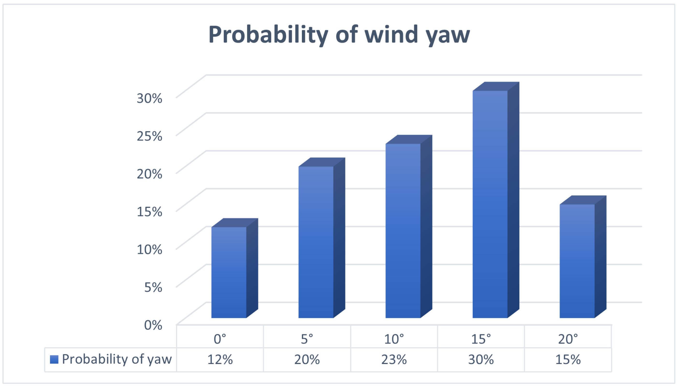Data from [21] were clustered. The low share of yaw angles >20° was not taken into account further. Note that 45% of the wind yaw is seen at angles higher than 10° with a calculated average yaw angle of 10.8°. This average value was later used for the Average CdA Bike Split Model. For the Weighted CdA Bike Split Model the probability of wind yaw was evaluated with the weighted wind distribution presented by Mavic. Yaw angles were binned to simplify the calculation procedure; see Figure 9.

4.3. General Bike Split Model

By using the Nabla Flow CFD simulation tool AeroCloud, a dimensionless CdA coefficient at a flow velocity of $U_x$ of 10m/s was extracted. In addition, drag force $F_d$ at the specified yaw angle $\beta$ was also derived. These two parameters are sufficient to calculate the necessary power to overcome the aerodynamically drag. To have a more accurate estimation of $P_{total}$, we needed to add the rolling resistance $P_{roll}$, the power to climb $P_{elev}$ and mechanical losses $P_{mech}$ (mechanical losses of 3% of the total power output were considered). Therefore, our model is summarized in Equation (1):

$$P_{total}=\left[\frac{1}{2}·\rho ·Cd{A}_{0^{\circ }}·U_x^3·cos\left(\beta \right)+c_r·m·g·U_x+\frac{m·g·dh·U_x}{ds}\right]·1.03$$

(1)

As velocity $U_x$ is represented in Equation (1) with the 3rd power, its accuracy is important. The temperature T also deserves a special discussion. A higher temperature results in a lower air density and cannot be neglected over the whole course of 180 km, nor can the change in altitude (which has the largest influences on the density and humidity). Sample calculations show that all effects—when taken together—result in changes in density of less than 2% Here we rely on data from one of the author’s races at IM Hawaii on 13 October 2018, stored in a TCX-file. (Bike computers record all relevant data, including distance, speed, elevation, etc., and store them in TCX files). For all the following calculations, an average air temperature of 27 °C (300.15 K) was used. The variables used were: $\rho$, density of air; $c_r$, rolling resistance coefficient; m, total mass; g, earth acceleration (9.81 m/s${}^2$); dh/ds, local slope of cycling path.

Other decisive factors are the elevation profile and the system mass of the cyclist and the bike. In this case, the system weighed 94 kg (83 kg athlete + 11 kg equipment). The elevation profile of the course was extracted from the TCX file, and the overall course was cut into 20 distinct segments; see

Table 3. IM Hawaii course segments.

	Total	Elevation	Elevation			Slope
Segment	Distance [m]	Point 1 [m]	Point 2 [m]	dh [m]	ds [m]	Angle [%]
1	3080	23	65	42	3080	1.4
2	3860	65	31	−34	780	−4.4
3	7530	31	95	64	3670	1.7
4	11,100	95	30	−65	3570	−1.8
5	11,800	30	65	35	700	5.0
6	39,900	65	107	42	28,100	0.1
7	49,800	107	34	−73	9900	−0.7
8	62,800	34	107	73	13,000	0.6
9	66,400	107	20	−87	3600	−2.4
10	79,600	20	90	70	13,200	0.5
11	84,900	90	52	−38	5300	−0.7
12	94,900	52	205	153	10,000	1.5
13	96,000	205	205	0	1100	0.0
14	106,000	205	52	−153	10,000	−1.5
15	111,300	52	90	38	5 300	0.7
16	124,500	90	20	−70	13,200	−0.5
17	128,100	20	107	87	3600	2.4
18	141,100	107	34	−73	13,000	−0.6
19	151,000	34	107	73	9900	0.7
20	180,000	107	23	−84	29,000	−0.3

. Segment 5, for instance, marks the short and steep climb at Palani road in Kailua-Kona, so it was not mixed up with another segment, as the average speed for a set power output at this climb is highly affected by $P_{elev}$ and therefore, by the system mass. Segment 12 and 14 will be highlighted as well. They mark the 10 km climb up to Hawi, and in reverse, the fastest part of the course: the 10 km downhill after the turning point. Looking closer at the table, we can also see that the long part on the Queen K Highway is symmetrical (segment 7 to 19) and can be regarded as rolling hills, as previously mentioned. In the downhill segments with negative slope angles $\alpha$, $P_{elev}$ is of particular interest. The so-called downhill slope force will add a negative value to the equation, and therefore allow one to increase the remaining values. Downhill segments are therefore much faster than flat or uphill segments with the same power output.

The last important parameter showing a high impact on the overall performance is the CdA value within the aerodynamic drag expression. As the focus of this work is the optimization of cycling posture to go faster, substantial savings can be seen within the improvement of the CdA value. Considering the different CdA values from the four positions, a bike split calculation was performed for each one of them to determine time saving on the IM Hawaii bike course. The cubic equation, shown in Equation (1), was solved by a simple fixed-point iteration for each increment ds from Table 3. The input power P was set to 300 W constantly. Equation (1) was then solved for $U_x$, and the increment in time dt for an increment in path ds was calculated via $dt=U/ds$.

4.4. Average and Weighted CdA Bike Split Model

For the Average CdA Bike Split Model, Equation (1) with constant yaw of 10.8° from Mavic’s case study was taken. Resulting values are shown in Figure 10. For the Weighted CdA Model the expression of $cos\left(\beta \right)$ is skipped, and a weighted CdA for 0° CdA was introduced instead. The power balance equation was therefore slightly modified; see Equation (2). The weighted CdA values were obtained by incorporating the corresponding probability for yaw; see in Figure 6. Both approaches are presented in Figure 10.

$$P=\left[\frac{1}{2}·\rho ·Cd{A}_{weighted}·U_x^3+c_r·m·g·U_x+\frac{m·g·dh·U_x}{ds}\right]·1.03$$

(2)

4.5. Discussion of the Bike Split Models

Both model predictions showed deviations of approximately 2.5%, resulting in approximately $6.5\pm 1.5$ min time savings. These deviations may be regarded as our model’s accuracy. Values are also shown in detail in

Table 4. Bike split prediction for weighted and averaged CdA model; time in hh:mm:ss.

Position	Average CdA Split	Weighted CdA Split	Differences	Deviation [%]
TT	04:12:48	04:07:11	00:05:38	2.23
DB	04:23:17	04:25:14	00:01:57	0.74
HD	04:41:15	04:57:48	00:06:33	2.25
HH	04:58:02	05:06:06	00:08:04	2.71

. The Average CdA Bike Split Model generally predicts slower times, except for the TT position due to the low change in CdA. The Weighted CdA Model, on the other hand, accounts for the lateral inflow angles, which is necessary on this course, because it is much more exposed to crosswinds than other IM courses.

Accordingly, the model favors positions that benefit from the sail effect at yaw angles.

Clearly visible is that the TT position shows the fastest performance in both models, with a predicted time of 4 h 12 min for the Average CdA Bike Split Model and a time of 4 h 7 min for the weighted CdA. Both are close to the bike course record, held by Cameron Wurf at a time of 4 h 9 min. The constant power output of 300 W resulted in an average speed of approximately 43 km/h in both models. Compared to the HH position, time savings of a little less than 1 h for the same power output can be achieved. Our distribution of the various drag components corresponds very well to measured distributions [9,23].

5. Discussion

5.1. Accuracy of the Complete Model

In addition to the mesh-dependency, a validation simulation for the HH position at 0° was run to investigate the calculated drag force and estimated aerodynamic power output and velocity prediction. Measured data from training rides were analyzed and compared to the simulations, and sufficient accuracy was obtained. Predicted average speeds by simulated CdA values are summarized in

Table 5. Predicted average speeds and comparison with tools Aerotune and Best Bike Splits.

CdA	Average	Weighted	Aerotune	BBS	Aerotune	BBS
Values	CdA [km/h]	CdA [km/h]	[km/h]	[km/h]	Deviation	Deviation
0.242	42.72	-	42.60	42.28	0.28%	1.03%
0.224	-	43.69	44.04	43.45	0.79%	0.56%
0.276	41.02	-	41.10	40.68	0.19%	0.83%
0.283	-	40.72	40.98	40.61	0.63%	0.27%
0.383	37.08	-	37.10	-	0.05%	-
0.412	-	36.27	36.47	-	0.56%	-
0.413	36.24	-	36.30	-	0.17%	-
0.450	-	35.28	35.48	-	0.55%	-

. Additionally, two reference simulations were performed by a German aerodynamic consultant company, Aerotune, Flensburg, Germany; and Best Bike Split from Training Peaks, LV, USA. As we can see in Table 5, the estimated bike splits deviate within a small range of less than 1% only (CdA values > 0.35, however, are not available in BBS simulation). Unlike our static and rather simplified model, the two reference tools use much more powerful algorithms and time-marching algorithms, and many more segments (>500).

These comparisons show that the actual velocity prediction methodology only introduces a minor additional uncertainty of less that 1%. Taking into account the mesh-dependency of CdA values, we estimate the accuracy of our complete procedure to be within engineering rages of 3%.

5.2. Comparing the Positions

As expected, on changing the cyclist’s posture, significant differences were observed. The aerodynamic drag coefficients (CdA) varied by more than a factor of 2, ranging from 0.150 (TT) to 0.328 (HH). Within a position, the CdA tends to increase slightly at crosswind yaw angles of 5–10° and decrease at higher yaw angles compared to a straight head wind. These findings were observed for the HH, HD and DB positions. While the HH and HD positions show poor performance in crosswinds, the DB position remains stable across yaw angles. The TT position, however, benefits from crosswinds and takes advantage of the sail effect.

The fastest bike split was calculated for the TT position (weighted CdA model) with a predicted time of 04:07:11, close to the IM Hawaii bike course record. The slowest bike split, on the other hand, was calculated for the HH position (weighted CdA model) with a predicted time of 05:06:06, and therefore, 20% slower than the TT position. These substantial time savings by roughly 60 min over the course of 180 km were found only by posture optimization. Within the two different bike split models, notable time differences of ±2.5% (5–8 min) were observed. The average CdA model generally predicts slower bike splits; however, it appears to be inaccurate over the whole course. The weighted CdA model, on the other hand, considers wind probability for each segment more accurately. Thus, wind yaw and the use of an appropriate model must be considered for bike split predictions.

6. Summary and Conclusions

The overall performance in a bike or triathlon race is highly dependent on the cyclist’s posture. Although the positioning on the bike is not static throughout the race, a clear trend is visible. By optimizing the cyclist’s posture, depending on the athlete’s bio-mechanical flexibility, from a comfortable to an aggressive position, the aerodynamic drag coefficient (CdA) can be reduced significantly by a factor of 2, which may result in substantial time savings of about 20%, or roughly 60 min over the course of IM Hawaii.

This is also visible in the flow wake structure. For the TT position, the wake is much smoother, whereas in the HH position, it seems to be much more irregular. More extended areas of reversed flow are accompanied by increased drag. Furthermore, within a position, the CdA tends to increase slightly at crosswind yaw angles of 5–10° and decrease at higher yaw angles compared to a straight head wind. These findings were observed for the HH, HD and DB positions. While the HH and HD positions showed negative performance in crosswinds, the DB position remains stable across yaw angles. The TT position, however, benefits from crosswinds and takes advantage presumably because of having the arms closer together, and therefore creating a smoother flow wake.

Our approach showed accurate agreement with prevalent bike split prediction tools, making a simple, mainly open-access-based workflow via iPhone, BLENDER and Nablaflow (AeroCloud) a competitive method for 3D performance analysis of a cyclist’s aerodynamics.

To further simplify and improve the process of geometry acquisition via scanning techniques, a machine learning method for deriving 3D triangulation from 2D pictures was tested. The open-source machine-learning-based tool ExPose was chosen. This approach proved to be feasible, but to improve its accuracy, model training by using more adapted body shapes seems to be necessary.

References

- Aerocloud. 2022. Available online: https://nablaflow.io/aerocloud (accessed on 10 July 2021).
- Wilson, D.G.; Schmidt, T.; Papadopoulos, J. Bicycling Science, 4th ed.; The MIT Press: Cambridge, MA, USA; London, UK, 2020. [Google Scholar]
- Blocken, B.; Toparlar, Y.; van Druenen, T.; Andrianne, T. Aerodynamic drag in cycling team time trials. J. Wind. Eng. Ind. Aerodyn. 2018, 182, 128–145. [Google Scholar] [CrossRef]
- Blocken, B.; van Druenen, T.; Toparlar, Y.; Malizia, F.; Mannion, P.; Andrianne, T.; Marchal, T.; Maas, G.J.; Diepens, J. Aerodynamic drag in cycling pelotons: New insights by CFD simulation and wind tunnel testing. J. Wind. Eng. Ind. Aerodyn. 2018, 179, 319–337. [Google Scholar] [CrossRef]
- Blocken, B.; Malizia, F.; van Druenen, T.; Gillmeier, S. Aerodynamic benefits for a cyclist by drafting behind a motorcycle. Sport. Eng. 2020, 23, 19. [Google Scholar] [CrossRef]
- Kyle, C.R.; Burke, E.R. Improving the racing bicycle. Mech. Eng. 1984, 106, 34–45. [Google Scholar]
- Lukes, R.A.; Chin, S.B.; Haake, S.J. The understanding and development of cycling aerodynamics. Sport. Eng. 2005, 8, 59–74. [Google Scholar] [CrossRef]
- Grappe, F.; Candau, R.; Belli, A.; Rouillon, J.D. Aerodynamic drag in field cycling with special reference to the Obree’s position. Ergonomics 1997, 40, 1299–1311. [Google Scholar] [CrossRef]
- Gross, A.C.; Kyle, C.R.; Malewicki, D.J. The aerodynamics of human-powered land vehicles. Sci. Am. 1983, 249, 126–134. [Google Scholar] [CrossRef]
- Defraeye, T.; Blocken, B.; Koninckx, E.; Hespel, P.; Carmeliet, J. Aerodynamic study of different cyclist positions: CFD analysis and full-scale wind-tunnel tests. J. Biomech. 2010, 43, 1262–1268. [Google Scholar] [CrossRef] [PubMed]
- Blocken, B.; van Druenen, T.; Toparlar, Y.; Andrianne, T. CFD analysis of an exceptional cyclist sprint position. Sport. Eng. 2019, 22, 10. [Google Scholar] [CrossRef]
- Giljarhus, K.E.T.; Stave, D.Å.; Oggiano, L. Investigation of Influence of Adjustments in Cyclist Arm Position on Aerodynamic Drag Using Computational Fluid Dynamics. Proceedings 2020, 49, 159. [Google Scholar] [CrossRef]
- Oggiano, L.; Leirdal, S.; Sætran, L.; Ettema, G. Aerodynamic optimization and energy saving of cycling postures for international elite level cyclists. In Proceedings of the 7th ISEA Conference, Biarritz, France, 3–6 June 2008. [Google Scholar]
- Debraux, P.; Grappe, F.; Manolova, A.; Bertucci, W. Aerodynamic drag in cycling: Methods of assessment. Sport. Biomech. 2011, 10, 197–218. [Google Scholar] [CrossRef] [PubMed]
- Crouch, T.N.; Burton, D.; LaBry, Z.A.; Blair, K.B. Riding against the wind: A review of competition cycling aerodynamics. Sport. Eng. 2017, 20, 81–110. [Google Scholar] [CrossRef]
- Crouch, T.N.; Burton, D.; Thompson, M.C.; Brown, N.A.; Sheridan, J. Dynamic leg-motion and its effect on the aerodynamic performance of cyclists. J. Fluids Struct. 2016, 65, 121–137. [Google Scholar] [CrossRef]
- Elfmark, O.; Giljarus, K.; Liland, F.; Oggiano, L. Aerodynamic investigation of tucked positions in alpine skiing. J. Biomech. 2021, 119, 110327. [Google Scholar] [CrossRef]
- Choutas, V.; Pavlakoe, G.; Bolkart, T.; Tzionas, D.; Black, M. Monocular Expressive Body Regression through Body-Driven Attention. In Proceedings of the Computer Vision ECCV, Glasgow, UK, 23–28 August 2020. [Google Scholar]
- Compressport. Aloha I Kona! 2018. Available online: https://www.compressport.com/ch/en/community/aloha-i-kona-n88/ (accessed on 10 September 2021).
- Barry, N. Real World Yaw Angles: PhD Design Engineer, Cannondale Bicycles. 21 June 2016. Available online: https://www.slowtwitch.com/Tech/Real_World_Yaw_Angles_5844.html (accessed on 24 August 2022).
- Cretoux, B. Yaw Angle Measurement in Real Conditions on Kona Ironman Course: Mavic Research Engineer. 2013. Available online: http://engineerstalk.mavic.com/en/yaw-angle-measurement-in-real-conditions-on-kona-ironman-course/ (accessed on 18 August 2021).
- Dirksen, F. Kona 2017 Recap. 21 November 2017. Available online: https://www.swissside.com/blogs/news/kona-2017-recap?locale=de (accessed on 24 August 2022).
- Isvan, O. Wind speed, wind yaw and the aerodynamic drag acting on a bicycle and rider. J. Sci. Cycl. 2015, 4, 42–50. [Google Scholar]