Article

Generating Activity-Based Mobility Plans from Trip-Based Models and Mobility Surveys

Department of Mobility Systems Engineering, School of Engineering and Design, Technical University Munich, Boltzmannstraße 15, 85748 Garching b. München, Germany
*
Authors to whom correspondence should be addressed.
Appl. Sci. 2022, 12(17), 8456; https://doi.org/10.3390/app12178456
Submission received: 20 June 2022 / Revised: 11 August 2022 / Accepted: 18 August 2022 / Published: 24 August 2022
(This article belongs to the Special Issue Advances in Smart Cities: Smart Grids, Buildings and Mobility Systems)

Abstract

:
Manifold applications in transportation system engineering rely on accurate modeling of human mobility demand. This demand is often represented by so-called mobility plans. Distinguished by their levels of aggregation, activity-based and trip-based models are the most prominent types of demand models in the literature. Macroscopic trip-based models are widely available but do not model mobility at the person level. In contrast, activity-based approaches simulate mobility microscopically but are complex and thus rarely available. The goal of this article is to present, apply, and validate an approach to generate activity-based mobility plans which microscopically reproduce real-world mobility demand but circumvent the complexity of activity-based approaches. To achieve this, existing trip-based models and mobility surveys are employed. Application results for car mobility in the city of Munich show that the obtained mobility plans are realistic on both a microscopic and a macroscopic level with regard to time, space, and activities. The presented approach can thus be considered appropriate for generating activity-based mobility plans whenever the development of a full-scale activity-based demand model is infeasible.

1. Introduction

Many applications in the area of transportation system design rely on accurate modeling of human mobility demand. So-called mobility plans constitute a prominent representation of such demand, which is needed to design new mobility systems for growing and modern cities using, for example, state-of-the-art traffic simulators such as Multi-Agent Transport Simulation (MATSim) [1] or Simulation of Urban Mobility (SUMO) [2]. A set of mobility plans includes information on the coordinates of origins and destinations, as well as departure and arrival times for every individual trip occurring within a population, timeframe, and spatial environment. An exemplary excerpt of one individual’s mobility plan is illustrated in Figure 1.
Synthesizing realistic mobility plans by means of abstracting human travel behavior within demand models has been the subject of many prior studies [3,4,5]. Distinguished by their levels of aggregation, activity-based and trip-based models are the two prominent types of demand models known today. Activity-based models produce mobility plans in which all movements are coherent within the frame of a microscopic entity, such as an individual person or car. In activity-based models, travel demand originates from the desire of individuals to participate in activities and is the result of trips taken to reach these activities [4]. Elaborate models of this type generate mobility plans that contain plausible mobility patterns and activity sequences on a microscopic level in addition to realistic, macroscopic traffic demand with regard to, for example, mileage, times, and locations. Activity-based models are based on simulating human behavior to explain and forecast traffic reactions to transportation policy or system changes, but this simultaneously makes them highly complex and expensive to implement, thus preventing established use [6]. As a result, activity-based demand models are scarcely available. In contrast, trip-based approaches are significantly more common and simpler to implement but fail to be realistic on a microscopic level. They realistically model traffic demand macroscopically by simulating aggregated traffic flows on network links [7].
The purpose of this work is to develop and validate a data-driven method for generating activity-based mobility plans that are realistic and coherent on an individual level without the complexity introduced by the behavioral nature of activity-based models. This places it between trip-based and activity-based demand models, as illustrated in Figure 2.
To this end, the output of an existing trip-based model is combined with data from a general mobility survey to arrive at a model that is capable of producing activity-based mobility plans that are microscopically coherent without losing macroscopic accuracy. This is achieved by merging the macroscopic characteristics of the general mobility survey with the microscopic and location-specific traits of the trip-based model to remodel the statistical properties of the input data without the explicit consideration of dynamic system behaviors that initially led to the observations within the input data sets. Our model is thus empirical and does not provide any basis for extrapolation but is systematically easier to implement than activity-based demand models. The presented model is designed and tested using existing data and models for the city of Munich. Nevertheless, this approach is applicable to any situation in which both a trip-based model and a general mobility survey for the study area are at hand, and building a full activity-based demand model is infeasible or inefficient. To reduce application complexity, the model is confined to a single mode of transportation, a structurally homogeneous spatial environment, and weekdays. The main contributions of the approach presented in this article are as follows:
  • An assessment of state-of-the-art mobility modeling;
  • The identification of a research gap spanning between easy-to-implement, macroscopic trip-based models and complex, behavioral activity-based models;
  • An approach to efficiently generate activity-based mobility plans from existing trip-based models and mobility surveys;
  • Its application to the city of Munich;
  • An overview and validation of the obtained results.
The remainder of this article is structured as follows. The related literature, including insights into mobility plan generation, mobility modeling, and existing mobility data, is presented in Section 2. Based on the literature assessment, the research gap is subsequently identified in Section 2.2, before Section 3 introduces an approach to generate activity-based mobility plans from trip-based models and general mobility surveys. The presented approach is applied to the city of Munich, and the obtained results are presented and validated in Section 4 before a discussion and conclusion of the presented ideas finish the article at hand in Section 5 and Section 6, respectively.

2. The Related Literature and Problem Statement

Planners of transportation systems need to know how many goods or people have to be transported at what times across which locations to design suitable transportation solutions. This section provides an overview of the related literature on mobility models which have been developed for transportation system planning. Building on this literature review, a research gap is identified and converted into a problem statement, motivating the introduction of a novel data-based approach to mobility plan generation.

2.1. The Related Literature

Due to the importance of mobility insights, a large body of the literature and practical mobility studies is available today. In contrast to the technical transportation perspective, which focuses and builds on origin-destination matrices as a proxy variable for mobility demand, mobility studies, which are rooted in the social sciences, require information on the reasons for transport demand. Hence, the assessment of human needs that induce activity patterns, location choices, and decision making adds to the bigger picture of human mobility. The mobility data sets available as a foundation for mobility studies can be divided into two groups based on the type of data sources: trace data, providing the locations of individual entities, and survey data, providing the mobility schedules of individual entities [8,9,10]. Trace data, when mined from existing data like call detail records [11,12] or social media data [13,14], have large samples sizes ( n 10 5 ), but oftentimes, no information regarding activities or persons emitting the traces are available [8,9]. In cases in which trace data can be attributed to identifiable persons, privacy preservation is a major challenge [15]. Aside from mining, trace data can be purposefully created using global positioning system (GPS) trackers. This enables capturing sociodemographic data and activity purposes, yet the sample sizes are small due to the high incurred cost (commonly n 10 3 ) [9]. In contrast to trace data, the survey data results are from censuses or travel surveys. A fundamental element of survey data is sociodemographic information. Censuses provide static data about residential and employment locations as well as high-level mobility metrics, such as the average commuting distance [8,9]. Travel surveys contain detailed information about the respondents’ mobility, especially with regard to trip purpose, mode of transport, time, and distance [16,17,18]. Compared with trace data, survey data have the advantage of providing sociodemographic information as well as information about the conducted activities. Their disadvantages are the high incurred effort, a coarse geospatial resolution to maintain anonymity, and dependence on the reporting accuracy on human memory [8,9]. The high effort additionally leads to them being infrequent and reflecting transportation changes with a delay [11].
Aside from mobility data collection through, for example, tracing and surveying, the identification of movement and behavioral patterns in raw data and the subsequent abstraction of such patterns allow for mobility forecasting and extrapolation. Partial models of mobility patterns include, among others, driving willingness models [19,20,21,22,23], location selection models [5,12,14,24,25,26], detour behavior models [27,28,29,30,31,32,33], and models for activity scheduling [18,34,35,36,37,38,39,40]. Integrated models, aimed at modeling the overall movements of larger populations, are clustered into trip-based and activity-based mobility models. These are reviewed in the following sections.

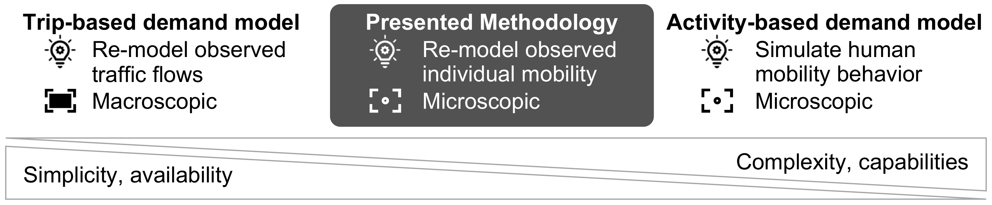
2.1.1. Trip-Based Mobility Models

The traditional trip-based model predicts aggregated traffic flows. It consists of four steps, namely trip generation, trip distribution, mode choice, and assignment. The modeled area is discretized into traffic analysis zones (TAZs), and the time of day is discretized into time bins. The trip generation step determines the number of trips originating from or terminating in each TAZ based on its sociodemographic and spatial attributes. During trip distribution, origins and destinations are linked to create trips. This step results in an origin-destination matrix, quantifying the traffic flow between any two TAZs. During mode choice, the trips are distributed onto the available modes of transport based on distance or travel time. The assignment step assigns the modal traffic flow between the TAZs to the transport network, resulting in a prediction of the aggregated traffic flow on each network link. Any interested readers can refer to Rasouli and Timmermans [41], who provide further information on the four-step model. Disaggregated versions of the traditional model differentiate between different groups of persons or even individuals to allow for a more realistic assignment of activities and modes, rather than assuming everyone in a TAZ behaves the same way. These modifications are made to overcome some of the traditional model’s disadvantages, such as the aggregation bias, yet do not provide spatially or temporally consistent mobility plans on a microscopic, individual level [42]. Tour-based models additionally prevent the traditional model’s knowledge loss and reduce inconsistencies. Rather than considering trips independently, they are combined into tours starting and ending at home. Thus, all trips can be traced back to households with their associated sociodemographic properties. Constraints ensuring the consistency of the sequence, location, time, and mode of trips may be introduced [7,43].

2.1.2. Activity-Based Mobility Models

Activity-based models aim to realistically represent the interdependencies of activities, times, locations, modes, and routes on a microscopic level. Most activity-based models share their two-step structure. They first generate a synthetic population to then generate schedules for each member or household within the population. A prototypical example for an activity-based model was presented by Bowman and Ben-Akiva [43]. Activity-based models are predominantly disaggregated.
Utility-based models were the first activity-based models to predict full-scale mobility plans. They simulate the human decision-making process as a two-step process of first generating a choice set and forming the solution space, followed by selecting the best alternative [42]. The decisions are modeled to imitate the human desire to maximize utility [41]. While the participation in activities yields a positive utility, the financial and temporal cost associated with traveling result in negative utility [3]. The research community further differentiates utility-based models into econometric models [4,43,44] and utility-based microsimulations [4].
Computational process models, occasionally termed rule-based, equal utility-based microsimulations in their focus on a complex search heuristic and the application of sequential decision-making processes, resulting in a specific solution. The two models differ in their decision-making processes: utility-maximizing approaches assume optimal decision making by humans, which has been deemed unrealistic by the authors of computational process models [41]. Hence, computational process models strive to select the first sufficient option rather than the globally optimal one [44].
Driven by the advances in the field of artificial intelligence, numerous models that leverage vast sets of trace data to train artificial mobility plan generators have recently emerged as new means to model human mobility. Some of these generative models generate artificial mobility plans that are indistinguishable from real ones. In contrast, others learn behavior from traces and allow the model developer to alter behavioral parameters. Applied techniques include generative adversarial networks [45], variational autoencoders [46], decision and regression trees [47], Markov models [48], hidden Markov models [49], and recurrent neural networks [50]. The downside of these approaches, however, is their reliance on large data sets for the target region to be modeled. Mining existing data sets to this end entails privacy challenges.

2.1.3. Hybrid Mobility Models

Moeckel et al. [5] identified a research gap between activity-based and trip-based mobility models. They presented a hybrid form in between these types that overcame some of the limitations inherent to trip-based models. Their framework, called Microsimulation Transport Orchestrator (MITO), models the trip demand of individual persons using activity-based methods, yet the model is easier to implement than activity-based models. They thoroughly covered the entire mobility of the population (i.e., all modes of transport) in a large, heterogeneous area, including both dense urban and rural areas. However, this led to compromises with regard to trip assignment to reduce model complexity. Hence, while the trip generation is highly realistic on a disaggregated level regarding sociodemographic factors, and macroscopic traffic indicators are validated to represent the observed mobility behavior, the assignment is not necessarily spatially or temporally consistent on a personal level.

2.2. Problem Statement

While activity-based models achieve remarkably realistic levels in modeling human behavior in theory, the inherent complexity and implementation efforts simultaneously restrict them from widespread use in practice. As a result, there is a gap between the state-of-the-art research and general application [5,51]. In conclusion, the implementation efforts of activity-based models still outweigh the limitations of trip-based models in the eyes of many potential users, such as transportation researchers, city planners, and governmental authorities. Hybrid models such as the one presented by Moeckel et al. [5] opt to reduce the gap between trip-based and activity-based models while simultaneously retaining the induced implementation efforts at a manageable level. Nevertheless, existing hybrid models do not reproduce microscopically accurate results. As a result, mobility plans generated by these approaches may include virtual agents who are located in two places at once or conduct activities in unreasonable frequencies or orders.
In addition to hybrid approaches, the gap between the trip-based macrosimulations and activity-based microsimulations of human behavior also houses the potential for a second intermediary research domain that microscopically reconstructs mobility on a personal, vehicular, or household level for a singular scenario with regard to time and space. This domain differs from activity-based models by not modeling the behavior required to, for example, simulate the traffic response to policy changes such as congestion charges but still reproduce the existing mobility of individual entities in a consistent and realistic way while simultaneously retaining realistic macroscopic transport indicators. Compared with activity-based models, this significantly reduces the effort of applying the model while, at the same time, providing the same value to applications that need a realistic microscopic model of today’s traffic but do not require to model’s behavioral responses at all. This work presents an approach to filling the outlined gap by building a model on two different input data sets: an existing trip-based model reflecting accurate mobility behavior for the target region with regard to the macroscopic indicators and spatial resolution and a general mobility survey comprising information on the typical activity patterns of people representative of the population of the same target region. Utilizing these data sets as well as existing partial mobility models on, for example, driving and detour willingness, the presented approach fills the outlined research gap.
One possible application, forming the motivation for the contribution presented in this article, is the simulation of urban electromobility using a simulation framework presented by Adenaw and Lienkamp [52]. In this application, microscopically realistic mobility plans of individual battery electric vehicles are required to consistently simulate their state of charge and induced charging behavior. The respective approach is based on the hypothesis that future electric vehicle users behave exactly as today’s drivers of internal combustion engine vehicles do with respect to mobility behavior. To this end, the overall amount, length, and spatial distribution of car trips needs to be remodeled based on the status quo for the target region in order to evaluate the spatiotemporal infrastructure utilization in the future. Although real transport demand is known to be elastic and hence sensitive to, for example, price changes [53,54,55] which inevitably come with the switch to another propulsion technology, a ceteris paribus analysis of charging behavior helps to reveal the general influences of technological changes and serves to reduce the system complexity to a manageable level. In these kinds of circumstances, activity-based models are out of scope and trip-based, and existing hybrid models are also not applicable because the traceability of individual cars is not provided. Similar usages may be found in other areas of transportation engineering in which no explicit modeling of behavioral responses but a reconstruction of the status quo mobility demand is needed on both a microscopic and a macroscopic level. This is due to the practical motivation of charging infrastructure simulation that the approach presented in this study is evaluated through a case study in Munich and focuses exclusively on the reconstruction of car mobility. In consequence, all generated mobility plans ought to be diaggregated onto cars, in contrast to the more prominent disaggregation onto people. To the best of the authors’ knowledge, no similar approach of reconstructing micro- and macroscopic mobility behavior realistically on a personal, vehicular, or household level, other than the more complex and resource-intensive agent-based models, has been presented before.

3. Materials and Methods

This section introduces an approach to generating synthetic yet realistic mobility plans before Section 4 presents the results obtained from its case study application to the city of Munich. Section 3.1 clarifies the requirements, metrics, and scope of application considered in this article. Based on these considerations, suitable input data for the case study application are derived in Section 3.2. These input data consist of the outputs of an existing trip-based model for the city of Munich as well as a general mobility survey for the whole of Germany. The developed approach employing these input data sets to reconstruct mobility behavior within Munich, effectively closing the aforementioned research gap, is presented in Section 3.3.

3.1. Requirements, Metrics, and Scope of Application

Prior to developing an approach to generate activity-based mobility plans from mobility survey data and a trip-based model, the requirements, validation metrics, and a scope of application are to be defined. Figure 3 visualizes the aforementioned fundamental structure of the presented approach together with the applied requirements and metric categories. Starting with separate information on the population’s general mobility behavior, as given by a mobility survey, and the location-specific behavior, represented by a trip-based model, activity-based mobility plans are generated. These plans have to respect both the macroscopic mobility behavior, including a realistic frequency, order, and time of activities as well as the microscopically accurate choice of activity locations, and the spatial and temporal consistency of the plans.
We distinguish between two types of requirements for the solution approach: output requirements and data requirements. These are further specified in the following and provide a framework for the later validation of the obtained results.

3.1.1. Output Requirements

Three output requirements (Req 1 ) are imposed on the methodology to ensure that the generated mobility plans are qualitatively similar to those generated by full-scale activity-based models.
Output Requirements Req 1
The generated methodology is implemented to accomplish the following:
  • Req 1 a : generate microscopically consistent and feasible activity-based mobility plans;
  • Req 1 b : achieve realistic macroscopic mobility behavior with regard to the order, frequency, location, time, and duration of activities as well as the induced travel distances;
  • Req 1 c : differentiate by sociodemographic groups.
In Req 1 a , consistency refers “to the space–time constraints of the individual” and feasibility to the “temporal, spatial and institutional constraints set by the environment” [41]. The main challenge of Req 1 b is to simultaneously exhibit the same realistic general mobility (frequency, order, and time) and location-specific behavior that the input data sets individually exhibit while not infringing on Req 1 a [48]. Therefore, the selection of activity locations must simultaneously show a realistic geographical distribution of locations (location-specific behavior) and a realistic distribution of driven distances (general mobility behavior). Since different sociodemographic groups are known to show different mobility behavior [56], sociodemographic characteristics are to be considered during this process Req 1 c .

3.1.2. Data Requirements

The aim to reduce complexity compared with activity-based models induces input requirement Req 2 a , stating that the methodology is to employ existing data. Req 2 b is induced by Req 1 c . To be precise, the input data consist of two existing data sets, as visualized in Figure 3. On the one hand, this requires a general mobility survey for modeling general mobility behavior (e.g., sequence and duration of activities, as well as drive times and distances of trips between activities). On the other hand, this requires a trip-based model to provide a synthetic population and model location preferences specific to the region for which activity-based mobility plans are to be generated. Lastly, due to the fact that our approach is set to remodel the observed mobility behavior without any analytical modeling of behavioral aspects and system dynamics, all characteristics relevant to the respective application within which our model is to be applied need to be reflected by the chosen input data sets (i.e., the input data need to be representative of the already relaxed mobility behavior of the study area, timeframe, mode, and user group at both the microscopic and a microscopic level). The elasticities, push and pull, or substitution effects, as well as any other form of user or system interaction, are not explicitly introduced into the model but instead assumed to be indirectly reflected by the input data sets.
Data Requirements Req 2
The methodology is to employ input data that fulfills the following:
  • Req 2 a : already exists (i.e., not specifically created);
  • Req 2 b : contains sociodemographic characteristics;
  • Req 2 c : contains all microscopic and microscopic traits of the mobility behavior to be reflected.

3.1.3. Scope of Application

Due to the scope and initial motivation of this work, the presented methodology exclusively models a car’s mobility behavior. Additionally, it is limited to modeling one distinct and structurally homogeneous spatiotemporal environment (Lim 2 ) (i.e., the presented approach models trips by car in an area of homogeneous density of development and a specific point in time). It is hence not designed to extrapolate or be applied to scenarios in which, for example, regions with heterogeneous mobility behaviors such as rural or urban regions are within the study area for which mobility plans are to be generated. The spatiotemporal environment of the case study is an urban area on working days, namely the city of Munich.
Limitations per Design
The methodology is to be limited to the following:
  • Lim 1 : trips by car;
  • Lim 2 : one homogeneous spatiotemporal environment.
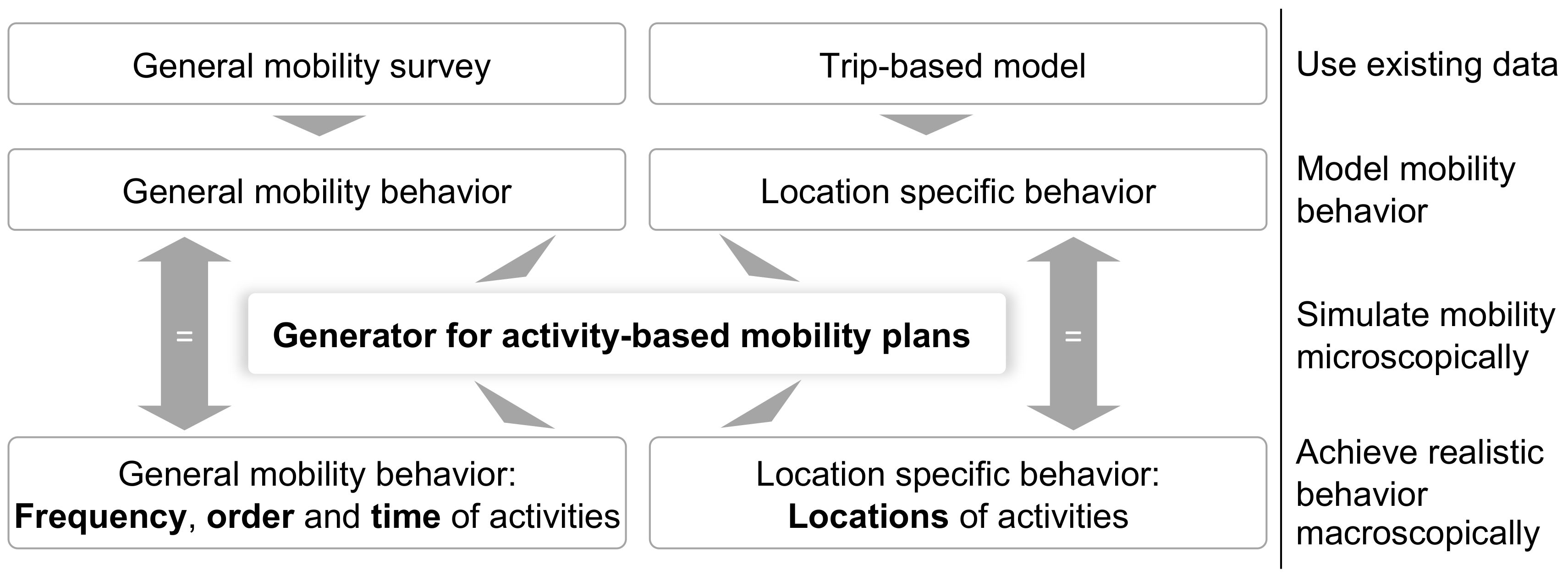
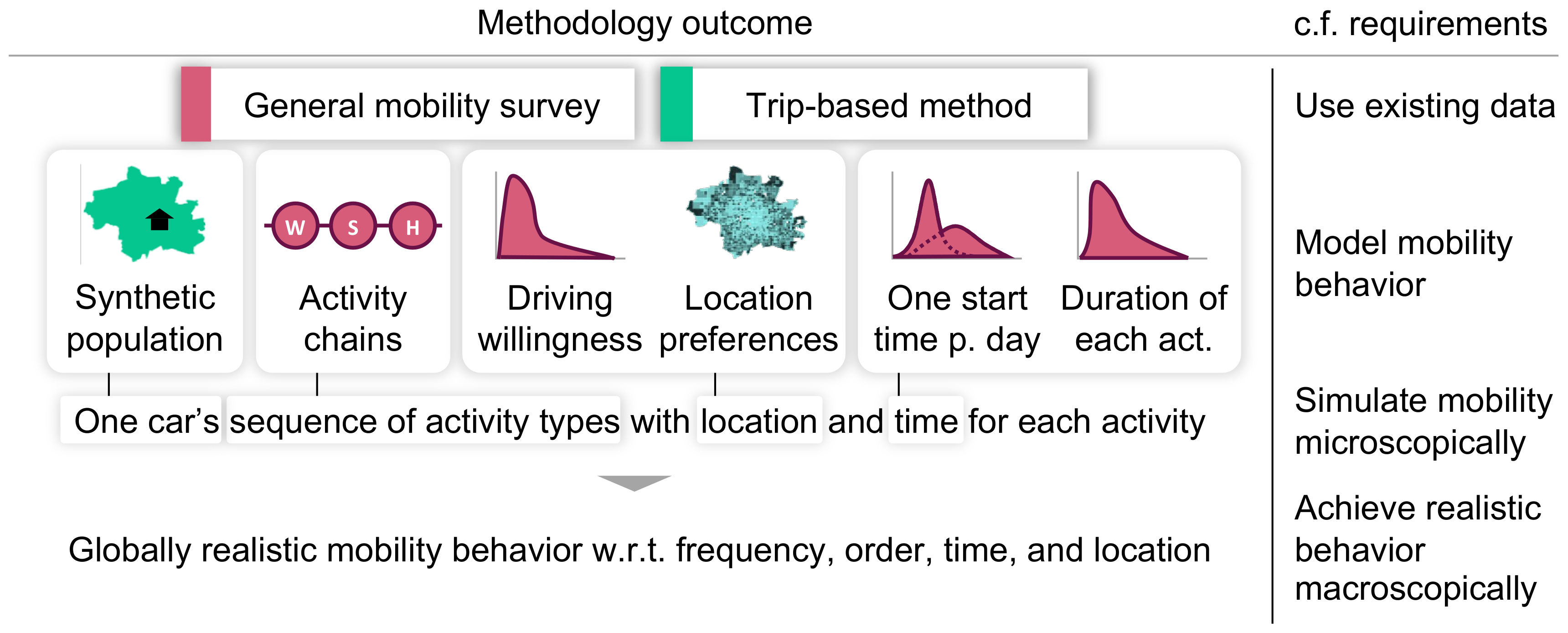
3.2. Input Data

Mobility behavior consists of two fundamental elements: general mobility behavior, which covers all characteristics such as the trip length independent of the context, and context-specific mobility behavior, which contains characteristics related to the observed situations (e.g., specific location preferences) [8]. Based on the requirements to employ existing data and to apply the methodology to the city of Munich, Mobilität in Deutschland (MID), a general mobility survey, and MITO, a trip-based model for the greater Munich area, were used as input data.
The mobility survey MID represents everyday mobility in Germany. The data consist of 960,619 trips conducted by 316,361 surveyed persons belonging to 156,420 households. Each household was tasked with reporting all trips of all household members on a randomly assigned date. The reported trip data comprise, among others, purpose, distance, origin and destination, time of departure and arrival, and mode of transport [16]. A weighting factor is provided for each trip to balance out the selection probability of sampling and achieve that relevant criteria such as age and sex are distributed equally in the sample and in the residential population of Germany.
MITO employs a microsimulation to individually model the mobility of households and persons that in turn constitute a realistic travel demand when aggregated. The model has been applied to the greater Munich area and provides location-specific preferences and a synthetic population for our application. Location preferences quantitatively compare the attractiveness of TAZs for a given activity type. The synthetic population contains households and persons for which travel demand is simulated. Aside from household composition and home location, it defines the destinations of mandatory trips for work and education purposes.
Based on the requirement to model car mobility on a weekday in the city of Munich, the input data had to be filtered and transformed from a person to a car perspective. To this end, the MID survey was filtered for trips in metropolitan environments on a regular weekday by a uniquely identifiable car. Out of 960,619 trips in MID, 2.9%, or 27,658 trips by 9053 cars, remained for further analysis. The strongest reductions were, applied in this order, the limitation to a metropolitan area of residency ( 82.4 % ) and trips where the reporting person was driving a car ( 72.0 % ). Each car was assigned a unique car identifier for further processing. Aside from the adjustments to the MID results, the MITO data were also preprocessed to meet this work’s requirements. First, the location preferences of MITO were filtered to only contain TAZs within the city limits of Munich. Second, the synthetic population was filtered to those living, working, and studying in Munich (1,223,532 people). Because of the car perspective employed in this approach, the synthetic population was also reduced to persons in possession of a driver’s license, ultimately resulting in 900,032 persons living in 624,571 households. Based on this, the synthetic car-population was created. Considering the number of cars per household and the limitation that a household could not simultaneously use more cars than members with driver’s licenses, the synthetic car population comprised 482,991 cars for which artificial mobility plans could be generated.

3.3. Approach

This section presents the developed approach for generating activity-based mobility plans from the data sets introduced before. Based on our focus on car mobility behavior, we defined the mobility plans as one car’s sequence of activity types with the location and time for each activity. This definition is depicted in Figure 4.
The figure also illustrates the operations and outcomes of the methodology, matching the requirements listed as known in Figure 3. Our approach consists of four generation steps. A synthetic (car) population for the target region is generated in the first step. Secondly, activity chains derived from the general mobility survey are attributed to the population. In a third step, locations are associated based on the information available from the trip-based input data before, in the fourth and final step, the time and duration of each of these activities are determined. The following sections elaborate on these steps. The resulting methodology is applied to the Munich case study in Section 4.

3.3.1. Initialize the Population

The car population contained static information about all simulated cars and thereby provided the foundation for generating mobility plans. The static information comprised everything that was assumed to not change throughout the simulation period for which mobility plans were generated [57]:
  • A car’s home location;
  • The driver’s static activities, such as work and education. When performed, they were always assumed to be at the same place and at the same time of day;
  • The driver’s work status.
The simulated car population was created by randomly sampling the desired number of cars from the synthetic car population known from Section 3.2 and assigning information on the static activities of the cars’ households’ inhabitants.
The data structure for the activity-based mobility plans was initiated by creating a table for each simulated car, comprising columns for activity type, time, duration, and location. Each car of the population started with a dummy activity to initialize the mobility plan. This fictitious “0th” activity set the start time and location of the mobility plan. The location of the 0th activity was set to the home location of the car. A second table was initiated to store the static information associated with the car.
Whether a car was used to get to work was based on whether the person drawn from the household had work information provided. This decision was thereby carried over from the trip-based model MITO, which is based on a realistic synthetic population. Hyperparameters p no _ worker and p worker were used to calibrate the share of the working population in case mobility plans were generated for samples small enough to skew the initially calibrated proportion of workers in the input population. If adjustments were not needed, then both were set to p = 0 . p no _ worker is the probability of replacing a working person with a non-working person, and vice-versa for p worker .

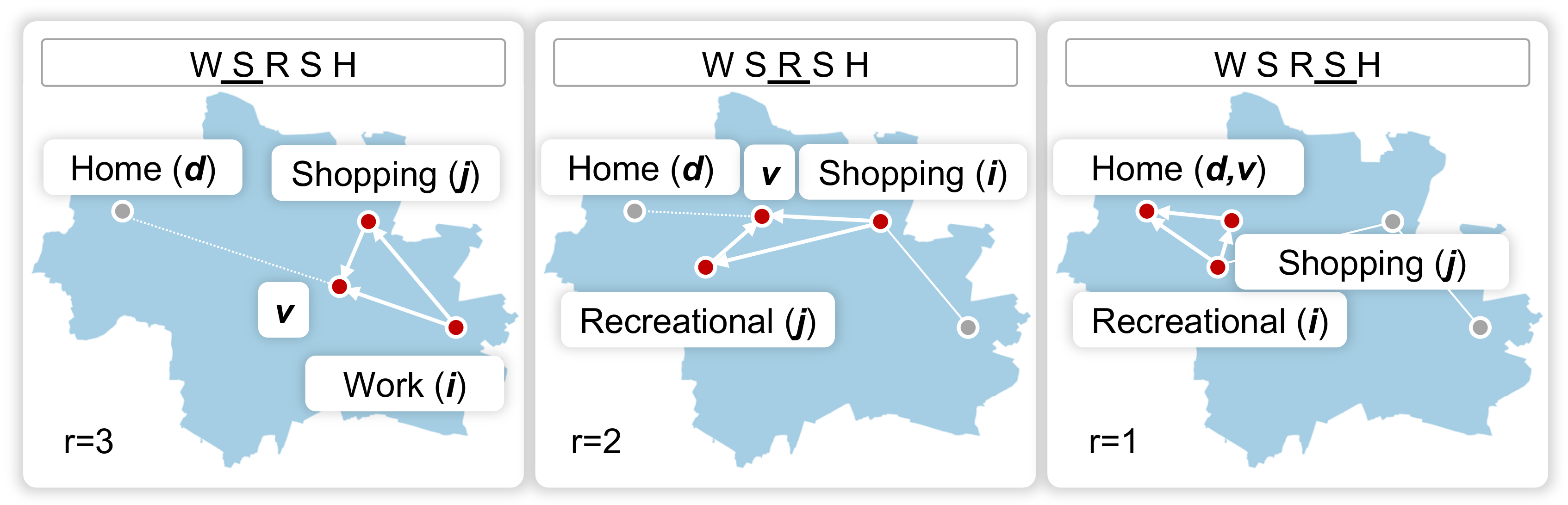
3.3.2. Derive the Activity Chains

An activity chain is a sequence of activity types throughout one day without any associated locations or timestamps. Due to the significant effort of creating realistic activity sequences [58] and the objective of this methodology being to facilitate application, activity chains were obtained from MID rather than being artificially generated. The main and secondary activities are distinguished within the activity chains. The main activities are the main purpose of leaving home as indicated in the mobility survey. Each roundtrip starting and ending at home therefore has exactly one main activity. All remaining activities are considered secondary activities. This information is used later on when locating activities in Section 3.3.3 and when assigning the times and durations of activities in Section 3.3.4. During location choice, the difference between the main and secondary activities induces different amounts of driving and detour willingness. In addition to the consideration of main and secondary activities, the relative weightings of the reporting persons from MID has to be respected in the derivation of activity chains. MID, like other general mobility surveys, uses weightings to correct for biases introduced by the participant selection frame, as opposed to the composition of the general population [16]. These weightings were carried over to the transformed car-based mobility survey and subsequently propagated to weightings of the aggregated activity chains.
Depending on the weighting factor of the obtained activity chains, sampling probabilities can be derived and exceptionally uncommon activity chains can explicitly be removed if desired for the respective application.
Using the presented approach, 1737 unique activity chains were identified within MID. MID includes a dedicated trip type for the “return from a previous activity”. Since the following activity type could not be deduced from this label, and due to its low share among all trip types ( 2.5 % ), all activity chains containing this type were removed. Furthermore, activity chains with less than five weighted occurrences were considered to be exceptionally rare and thus removed from the set of activity chains. A qualitative assessment of these rare activity chains showed that they were especially prone to implausibilities. These are, for example, the excessive repetition of activity types at home or work. fter all filtering steps, 173 unique activity chains with their respective probabilities remained.
Once the activity chains were generated and filtered as described before, each car was iteratively assigned an activity chain for each day of the desired simulation period. The result of this step was that each car then possessed a sequence of activity types for the simulated period of time. In multi-day simulation scenarios, some cars—mostly owned by the non-working share of the population—are expected to not be driven daily. To reflect this sociodemographic influence on activity selection, the activity chains were split into four groups based on whether or not they contained work activities and whether or not they started at home in the morning. While other studies distinguish more than two clusters in order to represent all relevant mobility groups within a population [59], the division into working and non-working populations was chosen to simplify the approach. This equals the methodology of Bhat [44] in that respect.
In order to model the difference between the working and non-working parts of the population, two additional hyperparameters were introduced into the model: p drive _ every _ day and p car _ driven . First, it was decided whether a car was driven every day based on the probability p drive _ every _ day . If this was not the case, then the second step was to decide daily whether the car was used or not with a probability p car _ driven and hence whether an activity chain was to be drawn for this day of the simulation.

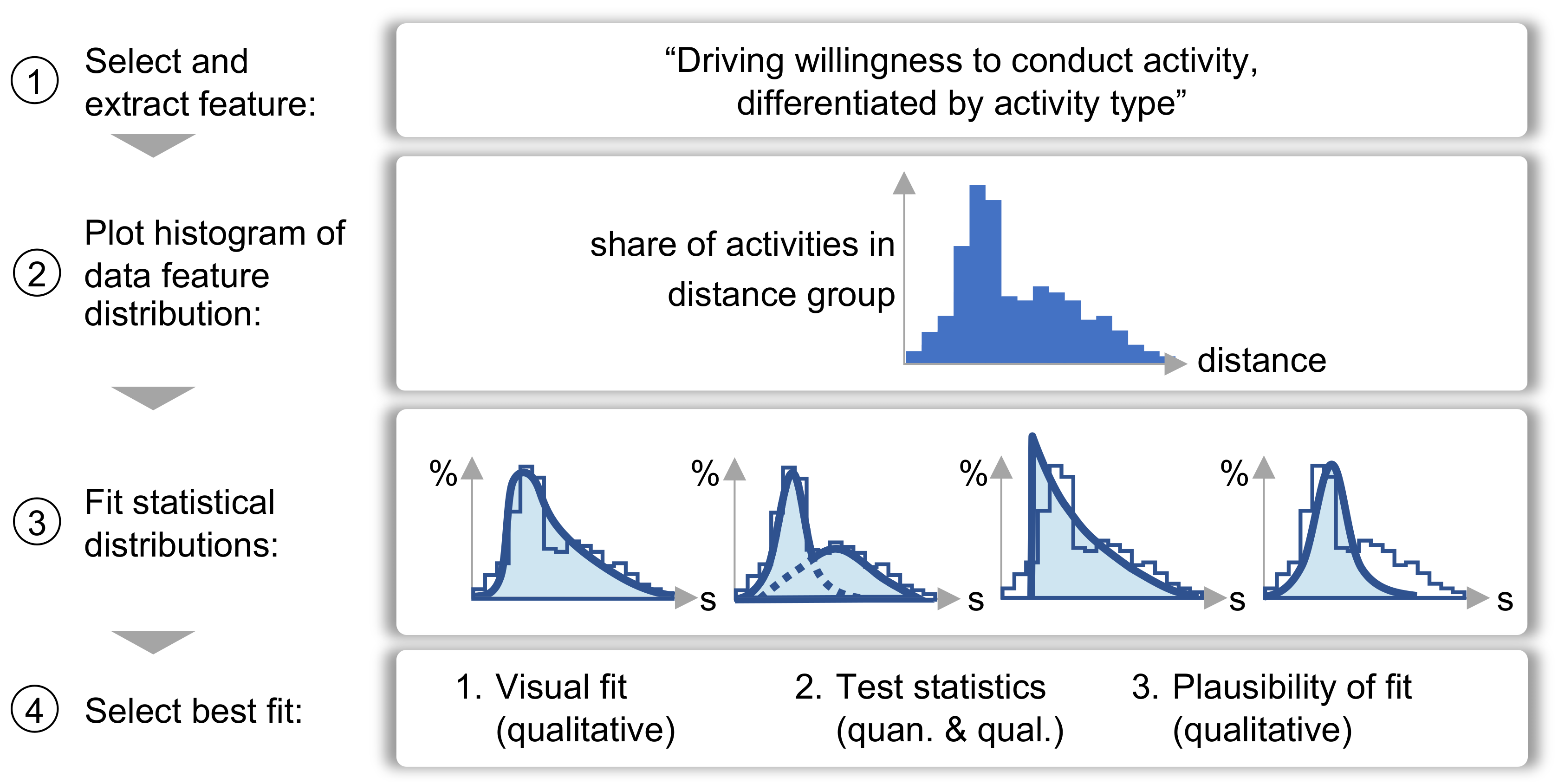
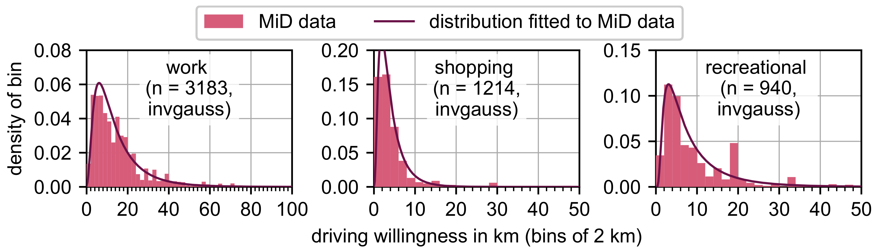
3.3.3. Assign Activity Locations

This section explains the assignment of TAZs to activities. As mentioned before, we distinguished between the main and secondary activities based on the survey results provided by MID. It was assumed that the distance to (and therefore the location of) the main activity does not depend on any other activities, which is why all main activities are located independently. Thereafter, all secondary activities would be located depending on the main activities’ locations. This resembles the approach of Hertkorn and Wagner [60] and Bowman and Ben-Akiva [43], who first assigned locations to activities on the highest hierarchical level—main activities in this context—and then, based thereon, the locations of activities on the lower or secondary hierarchical levels.
The locations of the static main activities were inserted from the car information table. The locations of all unassigned main activities were chosen based on a combined concept of TAZ attractivity and driving willingness. While, per definition, the locations of static activity types such as home and work always remained the same, the locations of non-static activity types such as shopping and recreation were chosen for each activity individually, (i.e., two main activities of the same activity type might not be located in the same location).
Driving willingness distributions model the willingness of persons to drive for a certain distance to conduct an activity. Driving willingness has been modeled by employing a variety of different distributions fitted with real-life trace data. Using this method, scholars considered gamma [19,21], Weibull [20], lognorm [20,21], exponential [22,23], and chi-squared [20] distributions. A clear consensus could not be identified. Hence, all aforementioned distribution types were fitted to the reported driving distances from MID using the following approach, as illustrated in Figure 5. For each activity type p occurring as a main activity, one probability density function (PDF) f p D ( d , p a r a m e t e r s p ) of driving willingness d over a continuous random distance variable D is created. The driving willingness of activity type p is the distribution of distances d i p (non-directed) of all trips p i ¯ and i p ¯ between home i and main activity p. In case of trips i p i ¯ , the considered distance is d p = 1 2 ( d i p + d p i ) .
Each distribution was determined by fitting a set of distribution types to the analyzed feature and qualitatively selecting the best fit based on three criteria:
  • Qualitative evaluation of the visual fit of the fitted distribution and a histogram of the analyzed feature, especially around the extreme values;
  • Quantitative (Kolmogorov–Smirnov test and Anderson–Darling test) and qualitative (QQ-plot) evaluation of statistical tests;
  • Qualitative plausibility check of whether the fitted distribution could be explained by real-life behavior, especially regarding overfitting.
The exemplary results are depicted in Figure 6.
To finally draw the locations of the main activities based on the driving willingness distribution and TAZ attraction, the probability Π j | i , p of choosing TAZ j for conducting main activity p when currently being in TAZ i is given by Equation (1):
Π j | i , p = w j | i , p l = 1 m w l | i , p
with
w j | i , p = c o n f j | i , p a t t j , p ,
c o n f j | i , p = d = d i j f p D ( d , p a r a m e t e r s p ) d d
= 1 F p D ( d i j , p a r a m e t e r s p ) ,
d i j = a dist d i j ¯ .
where m is the number of possible TAZs. This formula structurally resembles a multinominal logit choice model comparing all possible activity locations. Hence, locations were selected from all feasible alternatives. In line with econometric models, there was no pre-selection of alternatives [4]. Equation (1) is a modified version of the formula introduced by Moeckel et al. [5], who also determined activity locations based on a multinomial logit model that employs driving willingness and TAZ attraction. In contrast to their version, the mobility behavior conformance term c o n f j | i , p expresses how likely it is that one would drive at least the distance d i j to conduct activity type p. The conformance term is based on f p D and F p D , which are the PDF and cumulative distribution function (CDF), respectively, of the driving willingness distribution. D is the random continuous distance variable of these functions. The distribution type and parameters are specific to each activity type p and result from the distribution fitting process, and a t t is the TAZ-specific attraction, which corresponds to the number of places in a TAZ, where activity p can be performed, which was taken from MITO in our application. Meanwhile, d i j is the road distance between the centroids of TAZ i and j, approximated by the direct line distance d i j ¯ and a dist , a constant factor to approximate the road distance based on the direct line distance that is used to avoid routing and hence reduce the model complexity.
In reality, the selection of activity locations is a trade-off between the benefit of visiting a location and the effort of getting there [5]. Equation (1) models this behavior by rewarding an attractive TAZ ( a t t ) and penalizing long distances ( c o n f decreases with an increasing distance). Moeckel et al. [5] penalized the displeasure of transport by an exponential distance function. Hence, short distances are strictly favored over long distances. Our methodology, however, applies the probability of driving at least the considered distance. This models the trip’s conformance with observed mobility behavior, which decreases with the distance. The probability is calculated by integrating the driving willingness PDF over the interval from the considered distance to infinity. This slightly different approach was chosen to enforce that the simulated driven distances followed the same distribution as the underlying general mobility survey and allow different activity types to have different distribution types. This came at the cost of not modeling a human desire: the location choice was not constrained by the displeasure of driving but was statistically remodeled based on the observed distributions. This is more similar to trip-based methods than activity-based methods.
Following the assignment of the main activities’ locations, the secondary activities’ locations were assigned. The process for secondary activities differs from the one for main activities. This employs a concept of detour willingness instead of driving willingness while simultaneously respecting that there may be multiple secondary activities instead of a single main activity. As with driving willingness distributions, detour willingness distributions are used to quantify the willingness of persons to take a detour of a certain distance off of the direct route between home and a main activity to conduct a secondary activity. In our approach, detour willingness distributions were determined using the same distribution fitting approach as that for the driving willingness distributions. For each activity type p occurring as a secondary activity, one PDF f detour , p D ( d , p a r a m e t e r s p ) of a detour distance d over a continuous random distance variable D is created. This willingness was assumed to depend solely on the activity type of the considered secondary activity. The detour willingness of activity type p is derived from triangular trips i p j i ¯ originating from and ending at home i. In the case of the absolute detour distance, it is a distribution over detours d detour , p | i , j and is calculated as follows:
d detour , p | i j = d i p + d p j d i j ,
where j is the main activity and p is the secondary activity [33]. The distances were assumed to be undirected (i.e., Equation (6) is equally applicable for triangular trips i j p i ¯ ). This assumption induced small inaccuracies, as in reality, the distances on typical street networks do depend on the direction.
To connect multiple secondary activities, an iterative approach was chosen, as illustrated in Figure 7.
The algorithm connects the secondary activities of all activity chain snippets, with these being defined as activity sequences starting with a main or home activity with a coordinate i , followed by at least one secondary activity (without a location yet) and ending in a home or a main activity with a coordinate d . The variable i will be reassigned in each step to represent the current coordinate of the agent. The detour associated with visiting a TAZ is not calculated based on the direct route between the current coordinate i and destination d but between i and the newly introduced virtual destination coordinate v :
v = i + 1 r ( d i )
where r is the number of remaining secondary activities in the activity chain snippet which have not yet been assigned a location. With this concept of virtual destination, the agent gradually gets closer to the actual destination. On the one hand, this ensures that moving further away from the actual destination—which would be an undesired behavior [27]—is unlikely. On the other hand, the gradual movement ensures that, in the case of long activity chain snippets, the agent does not end up in the proximity of the actual destination early to then rotate around it.
The probability Π j | i , v , p of choosing TAZ j to conduct a secondary activity p, causing a detour from the direct route between the current location i and destination location v, is
Π j | i , v , p = w j | i , v , p l = 1 m w l | i , v , p
with
w j | i , v , p = c o n f j | i , v , p a t t j , p ,
c o n f j | i , v , p = d = d detour , j | i v f detour , p D ( d , p a r a m e t e r s p ) d d
= 1 F detour , p D ( d detour , j | i v , p a r a m e t e r s p ) ,
d detour , j | i v = d i j + d j v d i v ,
d x y = a dist d x y ¯ .
The difference between this and Equation (1) is the use of d detour , j | i v and f detour , p D / F detour , p D instead of d i j and f p D / F p D . Exact coordinates need to be determined once all activities have been assigned to a TAZ. While the coordinates of the home and work locations are already known from the synthetic population, the coordinates of the secondary activities are drawn to occur randomly within their target TAZ to simplify the approach.

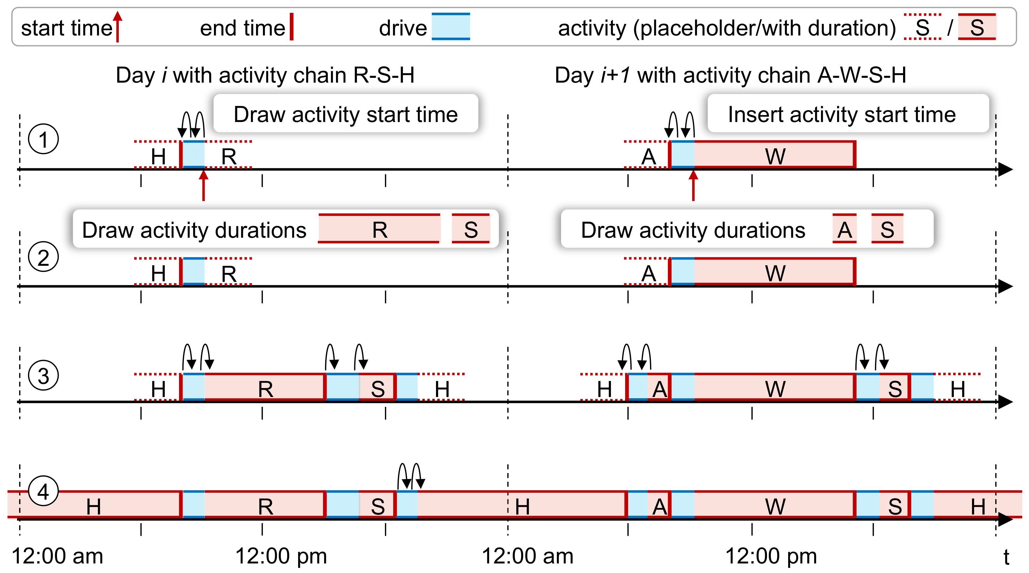
3.3.4. Determine the Times and Durations of the Activities

The time and duration of each activity can be determined once all activity locations have been determined, as the former depends on the drive time between activities, which in turn depends on the latter. The process of assigning a time and duration for each activity consists of four steps, as illustrated in Figure 8. To simplify the approach, it was assumed that the activities, activity start times, and activity durations were independent.
  • Step 1: Determining One Anchor Time per Day
The anchor time (one end time per day) locates a sequence of activities on the timeline. The first step depends on whether the start time information is available for any of the activities, which is the case if it is a static activity known from the synthetic population, such as working. If so, the start time of the first activity with available information is used as the anchor. If not, the start time of the day’s first activity is drawn from a start time distribution for the respective activity type. Using this start time, the end time of the previous activity is calculated and used as the next anchor time.
The start time distributions model the start times of activities. The distribution fitting process was the same as for the driving and detour willingness. For each activity type p (including the activity of being at home), one PDF f p T ( t , p a r a m e t e r s p ) of start time t over a continuous random time variable T is created. It is not further differentiated between main and secondary activities in order to prevent the creation of many small groups. The same applies to activity duration distributions. Since the start time behavior distribution is provided as a continuous PDF, probabilities can only be calculated for intervals and not for individual values, and those intervals are of l e n bin , s t a r t . We used bin lengths of 30 min ( l e n bin , s t a r t = 30 min ) for the start time distributions. This comparably large bin size was motivated by the distribution not being skewed toward the value 0 (midnight) and by the distribution covering a comparably large span of 24 h . This bin size represents a good balance of realistically representing the distributions’ major characteristics while not overfitting to the data.
The end time or anchor time of the preceding activity is calculated and inserted into the mobility plan based on the start time and the drive time to this activity. In the case of a drawn start time, a bin is drawn with a probability Π bin i :
Π bin i = t b i n i f p T ( t , p a r a m e t e r s p ) d t .
where f p T is the PDF of the start time distribution and T is the random continuous time variable. The distribution type is once more specific to the activity type p and the fitting parameters p a r a m e t e r s p , which results from the distribution fitting process. The center of the drawn bin is then taken as the start time. The drive times Δ t drive , x y between arbitrary locations x and y are calculated using the direct line distance d x y ¯ , a constant factor a dist for estimating the road distance based on the direct line distance, and the average velocity v avg , city of the analyzed urban area:
Δ t drive , x y = v avg , city 1 a dist d x y ¯ .
The average speed of cars in Munich, v avg , Munich = 32 km h , is applied for calculating the drive times [61]. The applied constant factor to approximate the road distance based on the direct line distance is a dist = 1.5 in the city of Munich [62]. In case both the activity start time and duration are available, the duration and the end time of that activity are already inserted into the mobility plan. In the case of work activities, the provided duration is the total daily duration of all work activities. Therefore, the provided work duration is distributed randomly to all of the day’s work and work-related activities.
  • Step 2: Drawing the Activity Durations
The activity duration distributions model the durations of activities. For each activity type p, including the activity of being at home, one PDF f p T ( Δ t , p a r a m e t e r s p ) of activity durations Δ t over a continuous random time variable T is created. The distribution fitting process is the same as for driving willingness. While the durations of the main and secondary activities might not exactly follow the same distributions, there is no differentiation between the main and secondary activities, as this differentiation would have to be made for the activity chains as well. This in turn would increase the number of unique activity chains and, at the same time, reduce the number of samples per unique activity chain. The probability Π bin i of b i n i is
Π bin i = Δ t b i n i f p T ( Δ t , p a r a m e t e r s p ) d Δ t .
where f p T is the PDF of the duration distribution and T is the random continuous time variable. The distribution type is specific to the activity type p which, along with the fitting parameters p a r a m e t e r s p , resulted from the distribution fitting process. The activity duration distributions have l e n bin , d u r = 5 min, which is the implicit resolution of the survey data. Out of the 15,815 trips for which duration information was provided, 90.2% or 14,260 trips had a reported duration of a multiple of 5 min, making it the most common multiple aside from the trivial multiple of 1 min. Due to most distributions being strongly skewed toward short durations, the bin size was chosen to be equal to the lower bound (i.e., the implicit resolution). Using the bin probability, a bin was drawn, and the lower edge of the drawn bin was used as the duration. The choice of the lower edge over the bin’s center was made to not underrepresent the bin containing the value 0. If the bin’s center were used, half of the bin containing 0 would be in the negative space and have a probability of 0. This choice would, however lead to a systematic underestimation of values, further motivating a small bin size to reduce the error.
The durations were drawn for all but the day’s last activities to not over-determine the schedule. Since there is one anchor time per day, n 1 out of n activities between two anchor times can have an independent duration. Furthermore, given that most mobility surveys cover 24 h starting at midnight, the duration of the last activity ending the following day is not known, (i.e., no duration distribution can be derived). The activity of being home was considered an activity like any other when it was encompassed by two non-home activities during the day. For this purpose, the duration distribution for this activity type was generated as well.
  • Steps 3 & 4: Calculating the Activity End Times for All Activities and Calculating the Day’s Last Activity’s Duration
The durations are iteratively inserted into the mobility plan, originating from the anchor time and calculating the drive times to or from the activities in each iteration. By calculating the drive times in each iteration, the algorithm is prepared for calculating time-of-day-dependent drive times, as the departure or arrival times are known when calculating the drive time.
As stated above, the duration of the day’s last activity cannot be drawn, but it is calculated in the fourth step from the penultimate activity’s end time, drive time to get there, and its own end time, which is on the following day.
Once the start times and durations were determined for all activities of all cars, cars with implausibly long total daily activity durations were removed. The total daily activity duration is the duration of all drives and activities in a day, except for the last activity. A total daily activity duration was considered implausibly long if it exceeded the available duration between the drawn adjacent end times. This case can easily be identified in the mobility plans because the duration of the problematic days’ last activity is negative in these cases. To reduce the approach’s complexity, this approach was chosen to solve the challenge of daily durations that exceeded the available duration between two end times.

4. Results and Validation

The presented approach was applied to the city of Munich. Table 1 lists the simulation parameters used to generate artificial workday mobility plans based on the presented methodology. In order to obtain a significant amount of mobility plans for evaluation, plans for 50,000 cars were generated for a 7-day period, of which 2 days were considered padding. This padding was used to eliminate the impact of edge effects on the beginning and end of the plans by removing the first and last day. Since a first test revealed a slight overestimation of the work activities, small nudges were applied using the p no _ worker parameter. Consequently, a car with work information provided was drawn to not belong to a working person with a probability of p no _ worker = 0.05 . The inverse probability remained p worker = 0 to not counteract the intended reduction of the working population. Intermediary test runs showed that the daily driving behavior of cars best matched the general mobility behavior judged by the MID study results when the remaining hyperparameters were set to p drive _ every _ day = 0.59 and p car _ driven = 0.4 . This means that the simulation assumed that approximately 59% of all cars within Munich were driven daily, whereas cars that were not driven daily were used on 40% of the days, or once every 2.5 d.
In the following, the obtained simulation results are shown in two separate sections. First, Section 4.1 provides an overview of the general mobility behavior reflected in the generated mobility plans, and the metrics employed in this section evaluate whether the order, frequency, and travel distances of the generated mobility plans were macroscopically realistic, as imposed by Req 1 b in Section 3.1.1.
Indicators of the general mobility behavior were validated by comparison with data from the employed general mobility survey MID. Subsequently, Section 4.2 assesses the spatiotemporal quality of the generated mobility plans based on a comparison with the results from MITO and MID. The herein conducted comparison of locations, times, and durations of activities concludes the evaluation of Req 1 b .

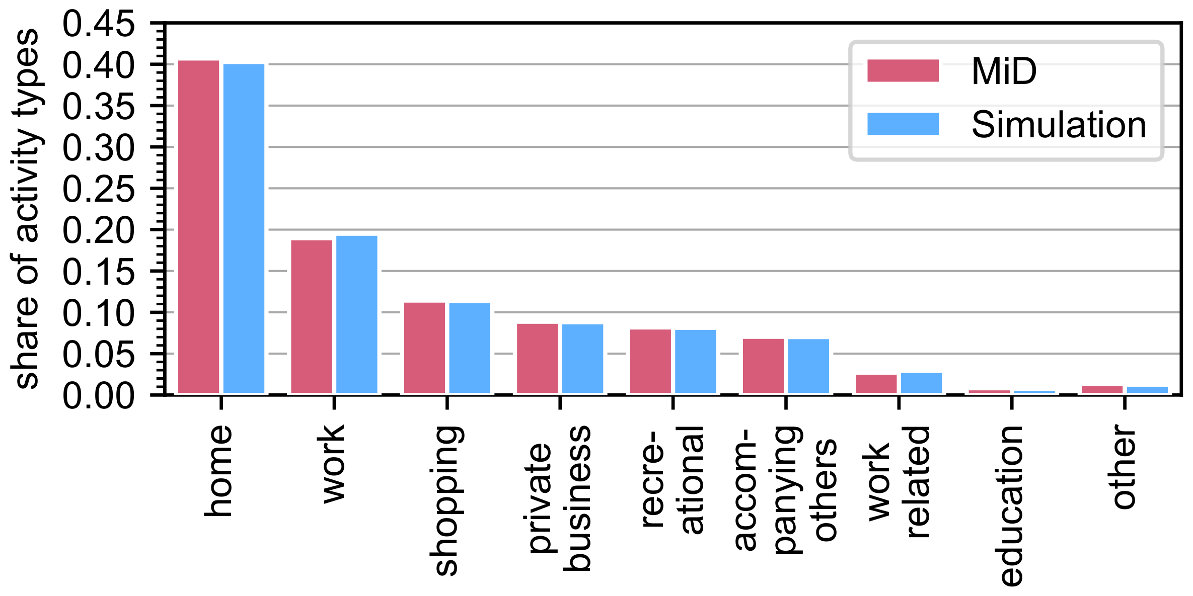
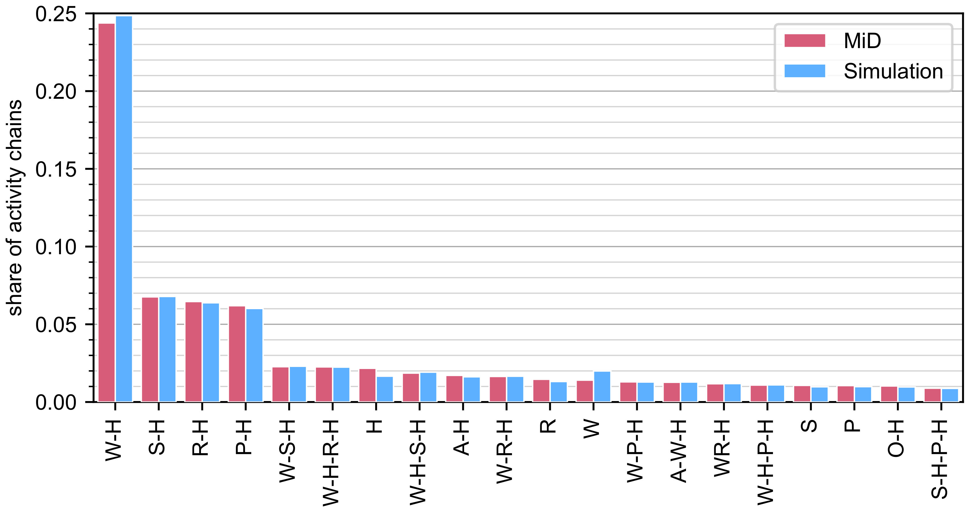
4.1. General Mobility Behavior

The urge to take part in activities steers human mobility behavior and induces travel demand. Hence, mobility models ought to accurately represent the types and prominence of different activities. Guided by the trip types used in MID and MITO, our model distinguishes nine different activities, namely “home”, “work”, “shopping”, “private business”, “recreational”, “accompanying others”, “work related”, “education”, and “other”. Figure 9 depicts the relative share for each activity type for the simulated mobility plans and the reference given by the general mobility survey MID. In MID, the survey participants were asked to report all trips occurring within one day starting and ending at midnight. However, MID does not report activities; rather, it reports trip types. From these trip types, a subsequent activity type can be implied (e.g., a trip labeled “shopping” is interpreted to end in a shopping activity). Looking at the results, it is evident that both the ranking of activity types regarding their prominence as well as the absolute share of each activity type were accurately reflected within the simulation results. A slight over-accentuation of work and work-related activities was present in the simulation results but amounted to less than 2% in terms of the relative activity share.
Aside from the occurrence frequencies of individual activity types, the order of activities within the generated mobility plans is another important characteristic. Figure 10 shows the share of the most prominent daily activity chains within the generated mobility plans in comparison to their MID counterparts. Special attention is to be paid to the circumstance that the initial activity of each day was unknown from the MID survey. The only exception is if the reporting person was at home in the morning, since this was separately asked. To allow for a fair comparison with MID, all activity chains resulting from the simulation were clipped to exclude the initial activity. Hence, the activity chains presented in the figure are to be thought of as partial activity chains. Most of these partial activity chains can be expected to start with a home activity in both MID and our generated mobility plans, as validated further below. A comparison on the basis of these partial chains reveals that the generated activity chain frequencies closely matched the MID reference, with deviations in the single-digit percentiles.
Since the information of whether an activity chain started from home was excluded, Table 2 consequently validates the share of people returning to and starting their days from home in contrast to chains starting or ending elsewhere.
On a more aggregated level, the amount of activities per car and day as well as the daily driven distance per car and day served as measures for the macroscopic modeling capabilities of our approach regarding general mobility behavior. Figure 11 marks the findings regarding these central mobility indicators when comparing the simulation results with MID. Similar to the aforementioned mobility factors, the distribution of the number of daily activities closely resembled the MID findings. Regarding the daily driven distances, however, a slight underrepresentation of large mileages can be observed, resulting in a smaller mean of daily driven distances per car. This phenomenon is based on the fact that our model is restricted to the boundaries of the city of Munich, effectively reducing the maximum possible trip distances to approximately 40 k m . Nevertheless, the existing deviations remained, on average, below 5 k m per car and day. Hence, in addition to realistic activities, the model also delivered reliable traffic benchmarks. Because of their apparent impact on the daily distances and the successful validation of these, our parameter choices for v avg , Munich and a dist were implicitly validated.
Figure 12 serves to elaborate on another aspect of the traffic indicators. It depicts the share of traveled distances per activity type. It is striking that the share of the travel distances associated with work activities within our mobility model was smaller than expected, although the share of working activities was found to be slightly larger than that in the reference survey. This may be due to the fact that the study area was restricted to the city of Munich, resulting in the implicit omission of any commuting for work or work-related activities. As a consequence, the share of the trip distances for all other activity types was marginally overestimated by our model.

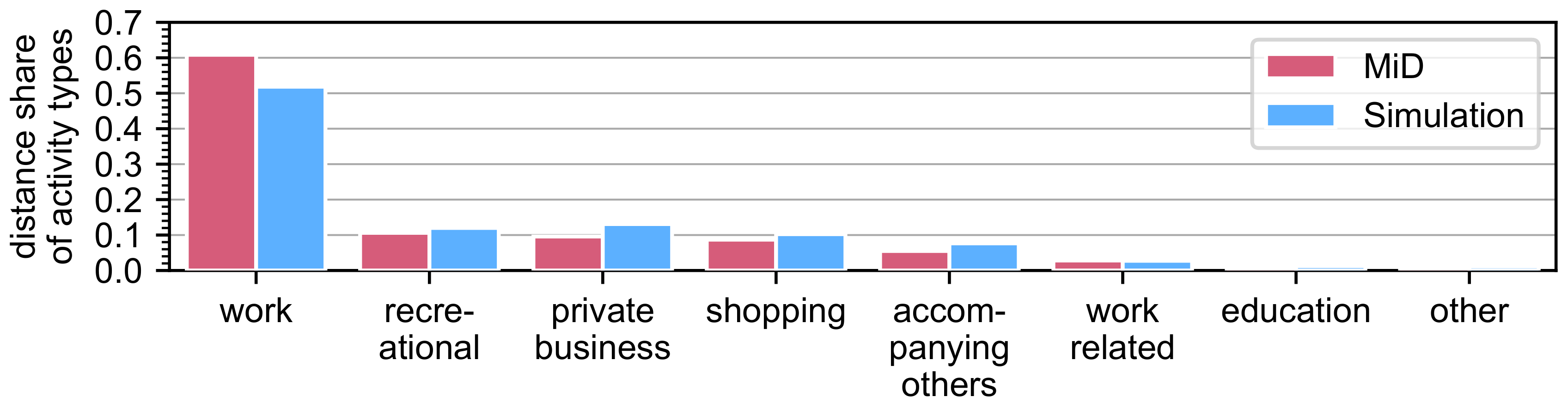
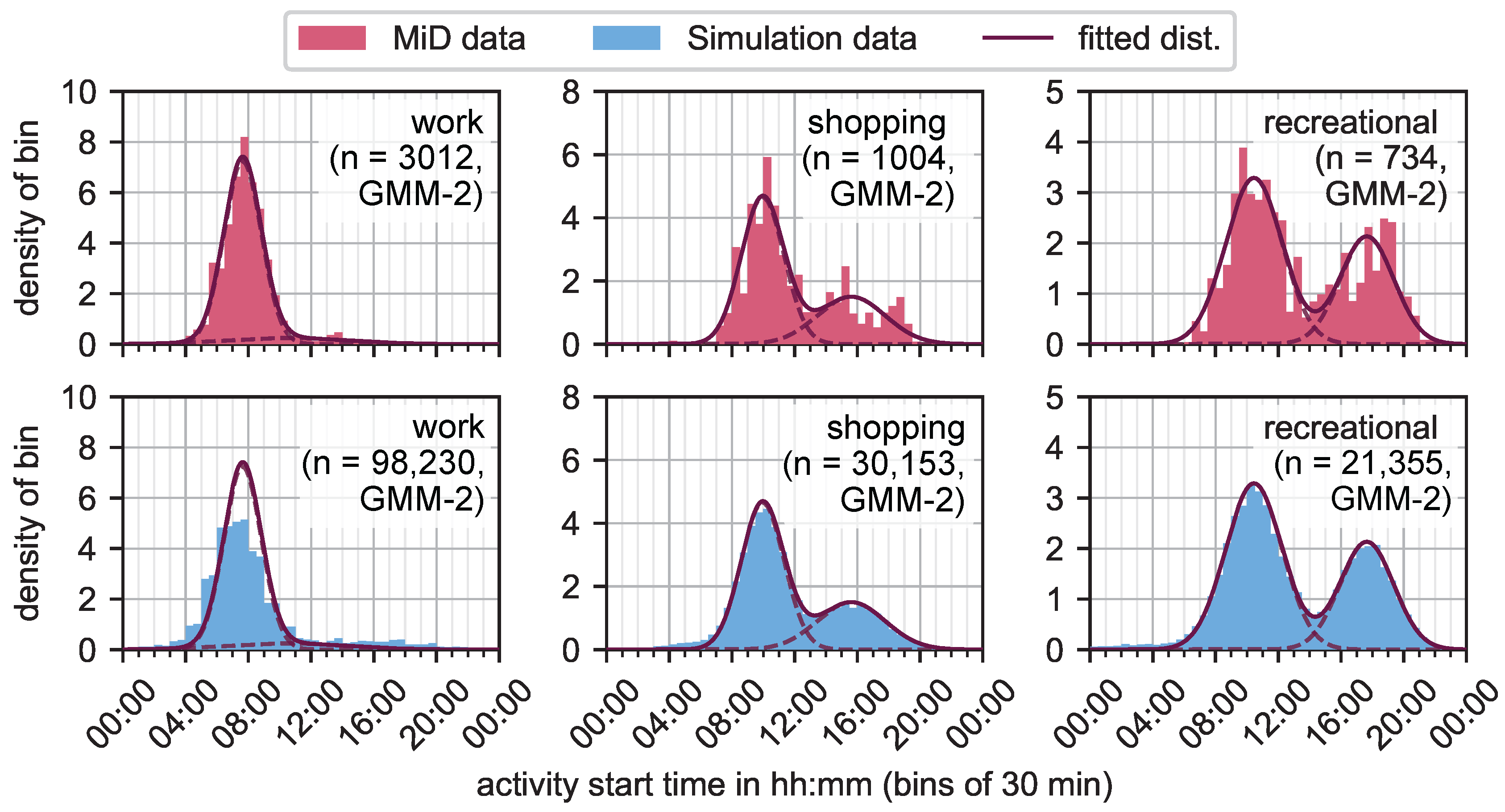
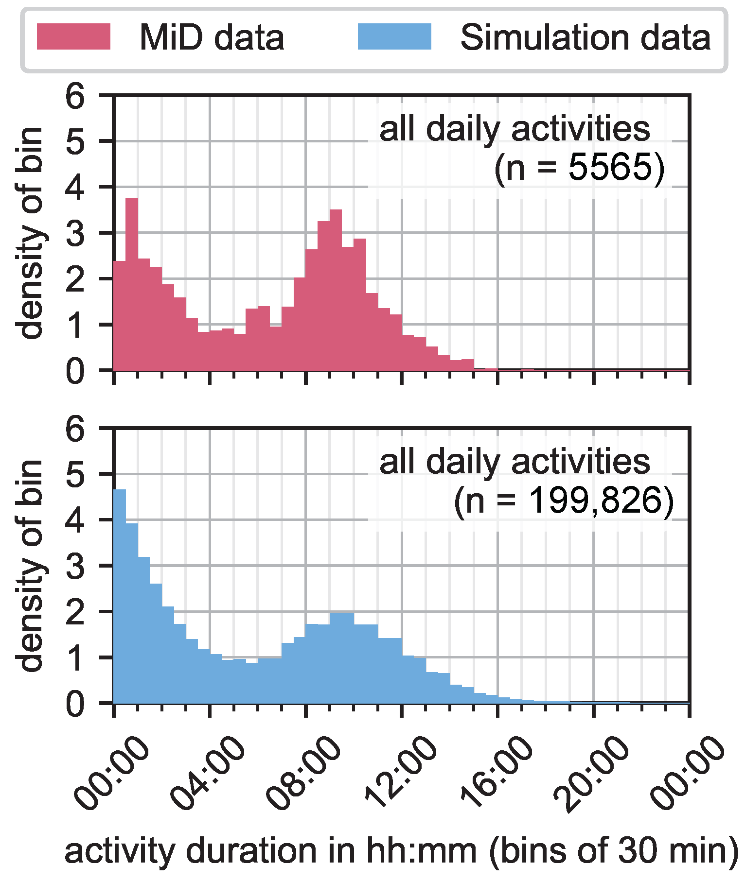
4.2. Spatiotemporal Mobility Behavior

This section presents the results regarding the spatiotemporal realism of the generated mobility plans. Figure 13 compares the start time distribution for work, shopping, and recreational activities in MID with their counterparts from our simulation. As expected, the generated start times accurately followed the fitted start time distributions and hence the original MID data. A slight exception was given by the work activities. The work activity distribution of our results exhibited a larger proportion of later work times. This deviation from MID is rooted in the fact that work activities are often main activities, serving as anchor times for their mobility plans based on the work time from the synthetic MITO population. It remains an open question whether MITO models the local Munich working behavior more accurately than the more aggregated MID survey.
The total activity duration per car and day is presented in Figure 14. A qualitative comparison of the activity durations reveals that the generated durations were mostly similar to those of the reference. It is to be noted, however, that the share of the short activity duration sums was larger than expected, resulting in overly short dwelling times at activity locations.
Aside from temporal considerations, the spatial modeling capabilities of the presented approach play an important role in its usability for transportation engineering tasks. In contrast to all previously mentioned statistics, MITO stepped up as the reference data set in this regard, since it focuses on the spatiotemporal modeling of mobility demand in Munich. Figure 15 can be used to assess whether the generated activities were distributed realistically among the different TAZs. The figure consists of four parts which are subsequently explained. The first row shows the distribution of visits per activity type according to the MITO reference. Work, shopping, and recreational activities are used to differentiate between the most important non-home activity types. Home locations are not shown since these were taken directly from MITO and thus matched the reference by design. In contrast, the distributions of non-home activities were a direct result of the presented location choice methodology and hence needed validation. For each TAZ, the absolute number of visits n v was divided by the total number of activities of the respective type N v to obtain the share associated with the TAZ. It can be seen that no single TAZ exceeded a share of 0.7% of any activity type. Considering the study area’s 1904 unique TAZs, a uniform distribution would result in 0.053% per zone. A logarithmic colorbar was used to better reveal the existing heterogeneity regarding activity distribution. Qualitatively, the city center and the outskirts can be recognized as the main working areas. Shopping is mostly focused around the city center, and recreational activities are distributed almost uniformly. The second row of the figure displays the same statistic for the simulated data set, qualitatively yielding the same results. To better access the differences between the reference and our results, a measure of error is needed. Hence, the symmetric mean absolute percentage error (SMAPE) was used as a measure for the deviations between MITO and our simulation. In this context, it is defined by Equation (17):
SMAPE = | n ˜ v , MITO n ˜ v , Simulation | n ˜ v , MITO + n ˜ v , Simulation
Herein, n ˜ v , MITO and n ˜ v , Simulation denote the share of visits n ˜ v = n v / N v per TAZ for a certain activity type. The third row of Figure 15 depicts the error distribution, conforming a first visual comparison of row one and two. The TAZs for which neither of the data sets counted any visits were left blank in this statistic. The vast majority of the remaining zones exhibited SMAPE values in the single-digit percentages, effectively validating a realistic distribution of activities by our approach. A more aggregated view on the same matter is shown in the fourth row of the figure. Here, the distribution of n v is summarized for both MITO and the simulation. Additionally, the distribution of the absolute errors | n ˜ v , MITO n ˜ v , Simulation | is depicted. The maximum number of visits per single zone m as well as the maximum absolute difference are also indicated. Please note that for comparability, all absolute numbers in the fourth row concerning MITO were scaled to match the simulation (i.e., they were multiplied by N v , Simulation / N v , MITO ). These figures support the conclusion that activities were successfully located by our approach, and because of small absolute differences, qualitatively similar visit distributions were found in comparison with the reference data set as well as similar maximum numbers of visits per individual zone.

5. Discussion

This section discusses the presented approach, the obtained results, and their implications from two different perspectives. First, Section 5.1 discusses the extend to which the presented approach fulfills the requirements set in Section 3.1, and Section 5.2 elaborates on the limitations of this work.

5.1. Requirement Fulfillment

Motivated by the research gap identified in Section 2.1, two output and two data requirements were imposed on the approach to be developed in Section 3.1. Following these requirements, the aim of the presented methodology is to generate microscopically consistent and feasible activity-based mobility plans (Req 1 a ) while simultaneously achieving a realistic macroscopic mobility behavior with regard to the order, frequency, location, time, and duration of each activity as well as the induced travel distances (Req 1 b ). Furthermore, the influence of sociodemographic factors on typical mobility patterns is to be respected (Req 1 c ). In order to reduce the complexity of the approach, it is required to operate on existing data only (Req 2 a ). These input data need to contain all necessary information, including the sociodemographic characteristics (Req 2 b ) considered in the fulfillment of Req 1 c . Within our validation case study for the city of Munich, we successfully fulfilled the input requirements Req 2 a and Req 2 b by employing the existing data sets MID and MITO. As a consequence, implementation of the approach did not involve any further data acquisition. It is worth noting that the presented methodology itself is not location-specific, in contrast to the data sets employed within our case study. The methodology can therefore be transferred to any study area for which equivalent input data sets are at hand. These data sets have to comprise a (synthetic) population, an associated set of trips within the study region, as well as a general mobility survey to deduce a realistic macroscopic mobility behavior. Fortunately, such data sets are widely available since they are used in many transportation engineering tasks. MID, for example, covers the whole of Germany and may be representative for other areas within central Europe. Despite these principle advantages regarding generalizability, the approach is always reliant on a location-specific trip data set and artificial population. Due to its input requirements, it is not a model that can be applied without location-specific engineering efforts. Looking at the output requirements, it can be said that the generated mobility plans are microscopically consistent and feasible with real-life mobility behavior (Req 1 a ) while being macroscopically realistic (Req 1 b ) at the same time. This statement is backed up by the successful validation of activity shares, activity chains, the number of activities per car and day, the realistic start times and durations, as well as the faithful spatial distribution of the different activity types, as presented in Section 4. From a methodological perspective, microscopic consistency was achieved by sequentially planning the drive and activity pairs, and hence no two activities of the same car could take place simultaneously in different locations. Each drive started where the previous one terminated. By design, no two consecutive activities were in the same place, ensuring that there was an actual drive between activities. Cars exceeding the available time (i.e., having activities longer than the time between two start times) were excluded from the simulation. Spatial feasibility was ensured by applying distance and drive time proxies, which resulted in trip distances and drive times that were between Google Maps’ estimates for low- and high-traffic scenarios. Hence, the travel speed was realistic as well. Temporal feasibility of individual activities was ensured by drawing from a distribution fitted to real activities, but the total daily activity duration was not ensured by design. Unrealistically long days may have occurred as a result, but they were filtered out. Institutional feasibility was not ensured by design either (e.g., shopping activities did not always take place during regular opening hours), though usually, this was because they were drawn from a respective distribution of shopping start times that statistically respected opening hours. The traveled distances per car and day and the work distance share among all activities were found to be underrepresented due to a small share of longer trips. This can be explained by the strict distance limit on the simulated cars imposed by not leaving the city limits. The underestimation of work’s distance share affirms the observation that the underrepresentation of long distances predominantly affects work trips, which is plausible considering the significant share of people commuting to places outside of Munich in reality. With these slight restrictions, the resulting mobility plans can be considered generally realistic, and the induced modeling complexity remains manageable. Specifically, it is smaller than the efforts entailed by building a full-scale activity-based model. This is due to the fact that only four hyperparameters are used within our model, and no explicit behavioral modeling is needed aside from the fitting of statistical distributions to ensure realistic mobility behaviors. In addition, the needed input data sets are pervasively available in urban regions. Nevertheless, some limitations remain. These will be discussed in the following section.

5.2. Limitations

The most apparent limitation of this work is given by its exclusive focus on car mobility. No other mode is considered by the employed methodology. This focus was set by design (Lim 1 ) because of the initial motivation that led to the development of the presented framework and the overall scope of this work. The question of whether and to what extent the presented methodology is generalizable to multi-modal mobility behavior remains unanswered. It is to be suspected, however, that the inclusion of multiple alternative modes of transport will incur additional modeling efforts, mainly due to the manifold interdependencies between mode choice, location choice, travel times, and activity durations. Another fundamental limitation of the work at hand is its applicability, which is restricted to homogeneous spatiotemporal environments (Lim 2 ). Based on the design of our approach and all means by which we validated it, no definite statement regarding its applicability to more heterogeneous areas that, for example, contain both urban and rural areas can be made. Regarding temporal mobility behavior, it has to be said that the existing approach is only fit to model weekdays. To enhance the capabilities of the methodology, the model could be extended to also include weekends. In addition to the existing mobility distributions for the working week, this would require replicating all distributions with the weekend data. Concatenating working weeks and weekends would allow one to significantly increase the simulation horizon to span a whole or even multiple weeks. However, the assumption of cars staying within an area of homogeneous mobility behavior does not hold as strong for weekends and longer time frames, interfering with the existing limitation to a restricted spatial domain. This leads to another potential enhancement of the capabilities: boundary conditions on the flow out of and into the area of homogeneous mobility behavior could enable modeling the strong geographical interdependencies of transportation systems without facing the complexity of them. These conditions can allow entities to temporarily leave the simulated areas and allow entities from outside to temporarily enter them without expanding the area of the simulation. The boundary condition would only determine at what time and, for example, with which state of charge cars return or enter. If the boundary conditions turn out to be realistically implementable, then the simulation of large areas of heterogeneous mobility behavior could be simplified by simulating many small areas of homogeneous mobility behavior and connecting them using boundary conditions. Another limitation of this work lies in the resolution with which sociodemographic influences were captured. Currently, the population is clustered into working and non-working people. A further differentiation promises to increase the quality and resolution of the results [63]. Additionally, to reduce the complexity of the approach, habitual behavior with regard to location selection was not modeled. This simplification is not assumed to impact the model’s validity, since it is of no relevance to the car whether the driver knows the destination as long as the distances are realistic.
A final but noteworthy limitation arises from the basic solution principal employed: the presented methodology is a data-driven and mostly statistical approach aimed at reproducing mobility behavior. It does so by incorporating both the general mobility behavior and the location-specific mobility behavior from two separate data sets without explicitly modeling human behavior. Hence, all mobility plans constructed by our approach merely represent the traits available in the input data, effectively merging two separate data sources Req 2 c . This procedure drastically reduces the modeling and application efforts in contrast to activity-based models while delivering similar outputs, but it prevents the usage of this model for any extrapolation or explanation of human mobility behavior. The desired scope of application of our model comprises ceteris paribus analyses of technological, organizational, and regulatory changes that are not expected to induce substantial changes to the population’s travel behavior. While this scope of application does offer various potential use cases, a more detailed and analytical modeling of elasticities, user behavior, and overall system dynamics is required for others. Therefore, our approach does not aim to replace or improve any kind of existing models but seeks to add to the toolbox of existing methods of mobility modeling, facilitating the options transportation engineers, researchers, and city planners can make use of when developing or evaluating new mobility solutions.

6. Conclusions

This article presents an approach to reconstructing activity-based mobility plans from trip-based data and a general mobility survey. The presented approach was developed, implemented, and validated with the goal of generating artificial mobility plans that are realistic yet efficient to obtain. It is applicable to any geographically limited area with homogeneous mobility behavior, and it was tested and validated using a case study in the city of Munich.
Based on a literature review on existing mobility models and the need for activity-based mobility plans in transportation engineering, this article identified a need for easy-to-implement mobility models capable of reproducing microscopically and macroscopically coherent mobility behaviors similar to activity-based models. While the capabilities of activity-based models with regard to the forecasting and explanation of mobility behavior are not needed for many applications, such as charging infrastructure simulations [52], their inherent complexities make them hard to implement and prevent them from being used pervasively. In contrast, the less complex trip-based or hybrid mobility models fail to model mobility behavior with the required microscopic accuracy. Hence, this article proposed a novel approach aimed at the reconstruction of status-quo mobility behavior from the output of trip-based models and general mobility surveys, with the general idea being that all information required to model mobility macroscopically and microscopically is conveyed by these two data sources and may be combined in a data-driven approach that is, for the most part, not reliant on any explicit behavioral modeling. While the resulting model does not offer the same forecasting and explanation potential as activity-based models and does not allow for any extrapolation of mobility behavior onto future scenarios, it is conceptually easier to implement and can be used in all cases in which the development of full-scale activity-based models is out of scope, but microscopic mobility modeling is needed. Within a case study conducted in the city of Munich, this approach proved to be both efficient and effective in creating activity-based mobility plans that were highly disaggregated yet did not fail to represent population-wide traffic indicators. The results obtained within the case study were based on data from MID and MITO, and they validated the suggested approach for the city of Munich, thus exemplifying that it is possible to generate realistic activity-based demands from trip-based models and general mobility survey data without adding the complexity of behavioral activity-based models.

Author Contributions

L.A. and Q.B. contributed equally to this work. L.A. conceived of the original idea to merge trip-based mobility plans with large-scale mobility survey data to generate activity-based mobility plans usable for mobility system simulation. Conceptualization, L.A. and Q.B.; methodology, L.A. and Q.B.; software, Q.B.; validation, L.A. and Q.B.; formal analysis, L.A. and Q.B.; data curation, L.A. and Q.B.; writing—original draft preparation, L.A. and Q.B.; writing—review and editing, L.A. and Q.B.; visualization, L.A. and Q.B. All authors have read and agreed to the published version of the manuscript.

Funding

This research was funded by the Technical University of Munich (TUM) in the framework of the Open Access Publishing Program.

Data Availability Statement

Within this study two major input data sets have been used and described: general mobility data from the MID study and an output data set from the MITO model. Restrictions apply to the availability of both of these data sets. MID data was obtained from the “DLR Clearing House Transport” and are available upon request at https://daten.clearingstelle-verkehr.de/279/ (accessed on 19 June 2022) with the permission of “DLR Clearing House Transport”. MITO data was obtained from the Professorship of Travel Behavior at the Technical University Munich and are available through this party on individual request. The output data generated by our model and presented in this study are not publicly available due to the possibility to reconstruct parts of the aforementioned third party input data sets from the results. Arrangements with all involved parties may be possible on request.

Acknowledgments

We would like to thank Rolf Moeckel and Carlos Llorca Garcia from the Professorship of Travel Behavior, who provided us with valuable views on mobility demand generation, artificial mobility plans, MITO, and SILO. Furthermore, we are grateful that they supplied us with the MITO data sets for use in the presented case study.

Conflicts of Interest

The authors declare no conflict of interest. The funders had no role in the design of the study; in the collection, analyses, or interpretation of data; in the writing of the manuscript, or in the decision to publish the results.

Abbreviations

The following abbreviations are used in this manuscript:
CDFcumulative distribution function
GPSglobal positioning system
MATSimMulti-Agent Transport Simulation
MITOMicrosimulation Transport Orchestrator
MIDMobilität in Deutschland
PDFprobability density function
QQ-plotquantile–quantile plot
SMAPEsymmetric mean absolute percentage error
SUMOSimulation of Urban Mobility
TAZTAZ

References

  1. Horni, A.; Nagel, K.; Axhausen, K.W. The Multi-Agent Transport Simulation MATSim; Ubiquity Press: London, UK, 2016. [Google Scholar] [CrossRef]
  2. Lopez, P.A.; Behrisch, M.; Bieker-Walz, L.; Erdmann, J.; Flötteröd, Y.P.; Hilbrich, R.; Lücken, L.; Rummel, J.; Wagner, P.; Wiessner, E. Microscopic Traffic Simulation using SUMO. In Proceedings of the 2018 21st International Conference on Intelligent Transportation Systems (ITSC), Maui, HI, USA, 4–7 November 2018; pp. 2575–2582. [Google Scholar] [CrossRef]
  3. Adler, T.; Ben-Akiva, M. A theoretical and empirical model of trip chaining behavior. Transp. Res. Part B 1979, 13, 243–257. [Google Scholar] [CrossRef]
  4. Bowman, J.L.; Ben-akiva, M. Activity based travel forecasting. In Proceedings of the Conference of Activity Based Travel Forecasting (Transcript of a Tutorial on Activity Based Travel Forecasting), New Orleans, LA, USA, 2–5 June 1996; Travel Model Improvement Program, US Department of Transportation and Environmental Protection: Washington, DC, USA, 1996; pp. 1–32. [Google Scholar]
  5. Moeckel, R.; Kuehnel, N.; Llorca, C.; Moreno, A.T.; Rayaprolu, H. Agent-Based Simulation to Improve Policy Sensitivity of Trip-Based Models. J. Adv. Transp. 2020, 2020, 1902162. [Google Scholar] [CrossRef]
  6. Moeckel, R.; Huntsinger, L.; Donnelly, R. From Macro to Microscopic Trip Generation: Representing Heterogeneous Travel Behavior. Open Transp. J. 2017, 11, 31–43. [Google Scholar] [CrossRef]
  7. Donnelly, R.; Erhardt, G.D.; Moeckel, R.; Davidson, W. NCHRP Synthesis 406: Advanced Practices in Travel Forecasting, 1st ed.; Transportation Research Board of the National Academies: Washington, DC, USA, 2010; pp. 1–90. [Google Scholar]
  8. Hess, A.; Hummel, K.A.; Gansterer, W.N. Data-driven human mobility modeling: A survey and engineering guidance for mobile networking. ACM Comput. Surv. 2015, 48, 1–39. [Google Scholar] [CrossRef]
  9. Barbosa, H.; Barthelemy, M.; Ghoshal, G.; James, C.R.; Lenormand, M.; Louail, T.; Menezes, R.; Ramasco, J.J.; Simini, F.; Tomasini, M. Human mobility: Models and applications. Phys. Rep. 2018, 734, 1–74. [Google Scholar] [CrossRef]
  10. González, M.C.; Hidalgo, C.A.; Barabási, A.L. Understanding individual human mobility patterns. Nature 2008, 453, 779–782. [Google Scholar] [CrossRef]
  11. Yin, M.; Sheehan, M.; Feygin, S.; Paiement, J.F.; Pozdnoukhov, A. A Generative Model of Urban Activities from Cellular Data. IEEE Trans. Intell. Transp. Syst. 2018, 19, 1682–1696. [Google Scholar] [CrossRef]
  12. Song, C.; Koren, T.; Wang, P.; Barabási, A.L. Modelling the scaling properties of human mobility. Nat. Phys. 2010, 6, 818–823. [Google Scholar] [CrossRef] [Green Version]
  13. Wu, L.; Zhi, Y.; Sui, Z.; Liu, Y. Intra-urban human mobility and activity transition: Evidence from social media check-in data. PLoS ONE 2014, 9, e97010. [Google Scholar] [CrossRef]
  14. Noulas, A.; Scellato, S.; Lambiotte, R.; Pontil, M.; Mascolo, C. A tale of many cities: Universal patterns in human urban mobility. PLoS ONE 2012, 7, e37027. [Google Scholar] [CrossRef]
  15. Bindschaedler, V.; Shokri, R. Synthesizing Plausible Privacy-Preserving Location Traces. In Proceedings of the 2016 IEEE Symposium on Security and Privacy, San Jose, CA, USA, 22–26 May 2016; IEEE: Piscataway, NJ, USA, 2016; pp. 546–563. [Google Scholar] [CrossRef]
  16. Nobis, C.; Köhler, K. Mobilität in Deutschland—MiD Nutzerhandbuch; Technical Report; Infas Institut für Angewandte Sozialwissenschaft GmbH: Bonn, Germany, 2018. [Google Scholar]
  17. Schneider, C.M.; Rudloff, C.; Bauer, D.; González, M.C. Daily travel behavior: Lessons from a week-long survey for the extraction of human mobility motifs related information. In Proceedings of the ACM SIGKDD International Conference on Knowledge Discovery and Data Mining, Chicago, IL, USA, 11–14 August 2013. [Google Scholar] [CrossRef]
  18. Raux, C.; Ma, T.Y.; Cornelis, E. Variability in daily activity-travel patterns: The case of a one-week travel diary. Eur. Transp. Res. Rev. 2016, 8, 26. [Google Scholar] [CrossRef]
  19. Shi, C.; Li, Q.; Lu, S.; Yang, X. Modeling the distribution of human mobility metrics with online car-hailing data-an empirical study in Xi’an, China. ISPRS Int. J. Geo-Inf. 2021, 10, 268. [Google Scholar] [CrossRef]
  20. Plötz, P.; Jakobsson, N.; Sprei, F. On the distribution of individual daily driving distances. Transp. Res. Part B Methodol. 2017, 101, 213–227. [Google Scholar] [CrossRef]
  21. Alessandretti, L.; Sapiezynski, P.; Lehmann, S.; Baronchelli, A. Multi-scale spatio-temporal analysis of human mobility. PLoS ONE 2017, 12, e0171686. [Google Scholar] [CrossRef]
  22. Bazzani, A.; Giorgini, B.; Rambaldi, S.; Gallotti, R.; Giovannini, L. Statistical laws in urban mobility from microscopic GPS data in the area of Florence. J. Stat. Mech. Theory Exp. 2010, 2010, P05001. [Google Scholar] [CrossRef]
  23. Jiang, S.; Guan, W.; Zhang, W.; Chen, X.; Yang, L. Human mobility in space from three modes of public transportation. Phys. A Stat. Mech. Its Appl. 2017, 483, 227–238. [Google Scholar] [CrossRef]
  24. Pappalardo, L.; Simini, F.; Rinzivillo, S.; Pedreschi, D.; Giannotti, F.; Barabási, A.L. Returners and explorers dichotomy in human mobility. Nat. Commun. 2015, 6, 8166. [Google Scholar] [CrossRef]
  25. Cuttone, A.; Lehmann, S.; González, M.C. Understanding predictability and exploration in human mobility. EPJ Data Sci. 2018, 7, 1–17. [Google Scholar] [CrossRef]
  26. Barbosa, H.; de Lima-Neto, F.B.; Evsukoff, A.; Menezes, R. The effect of recency to human mobility. EPJ Data Sci. 2015, 4, 21. [Google Scholar] [CrossRef]
  27. König, A.; Grippenkoven, J. Travellers’ willingness to share rides in autonomous mobility on demand systems depending on travel distance and detour. Travel Behav. Soc. 2020, 21, 188–202. [Google Scholar] [CrossRef]
  28. Zhang, W.; He, R.; Xiao, Q.; Ma, C. Research on Strategy Control of Taxi Carpooling Detour Route under Uncertain Environment. Discret. Dyn. Nat. Soc. 2016, 2016, 4702360. [Google Scholar] [CrossRef]
  29. Beojone, C.V.; Geroliminis, N. A Path to Take Passengers from Single to Shared Rides: A Study on Ridesplitting; Urban Transport Systems Laboratory: Ecublens, Switzerland, 2020; pp. 1–10. [Google Scholar]
  30. Santi, P.; Resta, G.; Szell, M.; Sobolevsky, S.; Strogatz, S.H.; Ratti, C. Quantifying the benefits of vehicle pooling with shareability networks. Proc. Natl. Acad. Sci. USA 2014, 111, 13290–13294. [Google Scholar] [CrossRef] [PubMed]
  31. Alonso-Mora, J.; Samaranayake, S.; Wallar, A.; Frazzoli, E.; Rus, D. On-demand high-capacity ride-sharing via dynamic trip-vehicle assignment. Proc. Natl. Acad. Sci. USA 2017, 114, 462–467. [Google Scholar] [CrossRef] [PubMed]
  32. Schneider, U. User perceptions of the emerging hydrogen infrastructure for fuel cell electric vehicles. In Proceedings of the ECEEE Summer Study, Belambra Les Criques, Toulon/Hyeres, France, 29 May–3 June 2017; pp. 867–876. [Google Scholar]
  33. Schneider, F.; Daamen, W.; Hoogendoorn, S. Trip chaining of bicycle and car commuters: An empirical analysis of detours to secondary activities. Transp. A Transp. Sci. 2021, 2021, 1–24. [Google Scholar] [CrossRef]
  34. Meister, K.; Frick, M.; Axhausen, K.W. A GA-based household scheduler. Transportation 2005, 32, 473–494. [Google Scholar] [CrossRef]
  35. Hilgert, T.; Heilig, M.; Kagerbauer, M.; Vortisch, P. Modeling week activity schedules for travel demand models. Transp. Res. Rec. 2017, 2666, 69–77. [Google Scholar] [CrossRef]
  36. Schneider, C.M.; Belik, V.; Couronné, T.; Smoreda, Z.; González, M.C. Unravelling daily human mobility motifs. J. R. Soc. Interface 2013, 10, 20130246. [Google Scholar] [CrossRef]
  37. Schlich, R.; Axhausen, K.W. Habitual travel behaviour: Evidence from a six-week travel diary. Transportation 2003, 30, 13–36. [Google Scholar] [CrossRef]
  38. Scherr, W.; Manser, P.; Joshi, C.; Frischknecht, N.; Métrailler, D. Towards agent-based travel demand simulation across all mobility choices—the role of balancing preferences and constraints. Eur. J. Transp. Infrastruct. Res. 2020, 20, 152–172. [Google Scholar] [CrossRef]
  39. Pas, E.I. Weekly travel-activity behavior. Transportation 1988, 15, 89–109. [Google Scholar] [CrossRef]
  40. Stopher, P.R.; Zhang, Y. Repetitiveness of daily travel. Transp. Res. Rec. 2011, 2230, 75–84. [Google Scholar] [CrossRef]
  41. Rasouli, S.; Timmermans, H. Activity-based models of travel demand: Promises, progress and prospects. Int. J. Urban Sci. 2014, 18, 31–60. [Google Scholar] [CrossRef]
  42. Feil, M. Choosing the Daily Schedule. Ph.D. Thesis, ETH Zurich, Zurich, Switzerland, 2010. [Google Scholar]
  43. Bowman, J.; Ben-Akiva, M. The Daily Activity Schedule Approach to Travel Demand Analysis. Ph.D. Thesis, Massachusetts Institute of Technology, Cambridge, MA, USA, 1998. [Google Scholar]
  44. Bhat, C.R.; Guo, J.Y.; Srinivasan, S.; Sivakumar, A. Comprehensive econometric microsimulator for daily activity-travel patterns. Transp. Res. Rec. 2004, 1894, 57–66. [Google Scholar] [CrossRef]
  45. Ouyang, K.; Shokri, R.; Rosenblum, D.S.; Yang, W. A non-parametric generative model for human trajectories. IJCAI Int. Jt. Conf. Artif. Intell. 2018, 2018, 3812–3817. [Google Scholar] [CrossRef]
  46. Huang, D.; Song, X.; Fan, Z.; Jiang, R.; Shibasaki, R.; Zhang, Y.; Wang, H.; Kato, Y. A Variational Autoencoder Based Generative Model of Urban Human Mobility. In Proceedings of the 2nd International Conference on Multimedia Information Processing and Retrieval, MIPR 2019, San Jose, CA, USA, 28–30 March 2019; pp. 425–430. [Google Scholar] [CrossRef]
  47. Drchal, J.; Čertický, M.; Jakob, M. Data-driven activity scheduler for agent-based mobility models. Transp. Res. Part C Emerg. Technol. 2019, 98, 370–390. [Google Scholar] [CrossRef]
  48. Pappalardo, L.; Simini, F. Data-Driven Generation of Spatio-Temporal Routines in Human Mobility; Springer: Berlin/Heidelberg, Germany, 2018; Volume 32, pp. 787–829. [Google Scholar] [CrossRef]
  49. Pozdnoukhov, A. Travel Demand Nowcasting; Technical Report 19; Department of Transportation: Washington, DC, USA, 2018. [Google Scholar]
  50. Kulkarni, V.; Garbinato, B. Generating Synthetic Mobility Traffic Using RNNs. In Proceedings of the 1st Workshop on Artificial Intelligence and Deep Learning for Geographic Knowledge Discovery, Los Angeles Area, CA, USA, 7–10 November 2017; pp. 1–4. [Google Scholar]
  51. Davidson, W.; Donnelly, R.; Vovsha, P.; Freedman, J.; Ruegg, S.; Hicks, J.; Castiglione, J.; Picado, R. Synthesis of first practices and operational research approaches in activity-based travel demand modeling. Transp. Res. Part A Policy Pract. 2007, 41, 464–488. [Google Scholar] [CrossRef]
  52. Adenaw, L.; Lienkamp, M. Multi-criteria, co-evolutionary charging behavior: An agent-based simulation of urban electromobility. World Electr. Veh. J. 2021, 12, 18. [Google Scholar] [CrossRef]
  53. Graham, D.J.; Glaister, S. Road Traffic Demand Elasticity Estimates: A Review. Transp. Rev. 2004, 24, 261–274. [Google Scholar] [CrossRef]
  54. Libardo, A.; Nocera, S. Transportation elasticity for the analysis of Italian transportation demand on a regional scale. Traffic Eng. Control 2008, 49, 187–192. [Google Scholar]
  55. Wardman, M. Price Elasticities of Surface Travel Demand A Meta-analysis of UK Evidence. J. Transp. Econ. Policy JTEP 2014, 48, 367–384. [Google Scholar]
  56. Luo, F.; Cao, G.; Mulligan, K.; Li, X. Explore spatiotemporal and demographic characteristics of human mobility via Twitter: A case study of Chicago. Appl. Geogr. 2016, 70, 11–25. [Google Scholar] [CrossRef]
  57. Arentze, T.A.; Timmermans, H.J. A learning-based transportation oriented simulation system. Transp. Res. Part B Methodol. 2004, 38, 613–633. [Google Scholar] [CrossRef]
  58. Auld, J.; Mohammadian, A.K. Activity planning processes in the Agent-based Dynamic Activity Planning and Travel Scheduling (ADAPTS) model. Transp. Res. Part A Policy Pract. 2012, 46, 1386–1403. [Google Scholar] [CrossRef]
  59. Jiang, S.; Ferreira, J.; González, M.C. Clustering daily patterns of human activities in the city. Data Min. Knowl. Discov. 2012, 25, 478–510. [Google Scholar] [CrossRef]
  60. Hertkorn, G.; Wagner, P. The application of microscopic activity based travel demand modelling in large scale simulations. In Proceedings of the World Conference on Transport Research (WCTR), Istanbul, Turkey, 4–8 July 2004; pp. 1–10. [Google Scholar]
  61. Durchschnittsgeschwindigkeit in Europäischen Städten. Available online: https://de.statista.com (accessed on 17 August 2022).
  62. Schröder, D.; Gotzler, F. Comprehensive spatial and cost assessment of urban transport options in Munich. J. Urban Mobil. 2021, 1, 100007. [Google Scholar] [CrossRef]
  63. Eagle, N.; Pentland, A.S. Eigenbehaviors: Identifying structure in routine. Behav. Ecol. Sociobiol. 2009, 63, 1057–1066. [Google Scholar] [CrossRef] [Green Version]
Figure 1. Exemplary mobility plan of all trips of an individual on one day. The last activity of the preceding day provides the work trip’s origin.
Applsci 12 08456 g001
Figure 2. The presented methodology is located between trip-based and activity-based demand models.
Applsci 12 08456 g002
Figure 3. Overview of input and output requirements on methodology.
Applsci 12 08456 g003
Figure 4. Definition of an activity-based mobility plan and outcomes of the methodology’s steps. Red and green elements belong to general and geospatial-specific mobility, respectively.
Applsci 12 08456 g004
Figure 5. Schematic illustration of the process of generating driving willingness distributions.
Applsci 12 08456 g005
Figure 6. Observed driving willingness (original weighted data) and fitted distributions with the best fit.
Applsci 12 08456 g006
Figure 7. Exemplary illustration of determining secondary activity locations for an activity chain with three secondary activities (from left to right). The activity assigned in the current step is underlined. The virtual destination v always lies on the direct line between the previously assigned activity location i and the destination d and is applied for calculating the detour. Bold arrows represent the distances applicable in the respective current step.
Applsci 12 08456 g007
Figure 8. Exemplary illustration of the four process steps of assigning an end time and duration to each activity. The red arrow in step one marks the drawn or inserted start time. Vertical red lines represent activity end times. Bent arrows illustrate that that element at the head of the arrow can uniquely be located on the timeline given the element the arrow originates from. Blue and red represent driving and activity, respectively. Drive times are exaggerated for illustrative purposes. Please note that the underlying mobility plan is not consistent with the assumption that a person either has work activities on all days (working) or on none (non-working), but it was chosen to illustrate both cases.
Applsci 12 08456 g008
Figure 9. Share of activity types. Comparison of simulation and MID.
Applsci 12 08456 g009
Figure 10. Share of partial activity chains. Comparison of simulation and MID. Activity types are abbreviated by their first letters (home = H, work = W, shopping = S, recreational = R, work-related = WR, private business—P, accompanying others = A, education = E, and other = O).
Applsci 12 08456 g010
Figure 11. Comparison of the simulation output with MID survey data in terms of daily distances and number of activities. (a) Number of activities per car and day. (b) Distance driven per car and day.
Applsci 12 08456 g011
Figure 12. Distance share among activity types. Comparison of simulation and MID.
Applsci 12 08456 g012
Figure 13. Start times of the first activity per activity type. Comparison of simulation and MID.
Applsci 12 08456 g013
Figure 14. Total activity duration per car and day. Comparison of simulation and MID.
Applsci 12 08456 g014
Figure 15. The heatmaps geographically compare activity locations of MITO and our simulation. The two rows from below validate whether the distribution of visits per TAZ is realistic.
Applsci 12 08456 g015
Table 1. Simulation parameters.
ParameterValueParameterValueParameterValue
n cars 50,000 Δ t 7 d Δ t p a d d i n g 2 d
p drive _ every _ day 0.59 p car _ driven 0.4 p no _ worker 0.05
p worker 0 a dist 1.5 v avg , Munich 32 km h
Table 2. Share of cars returning to and starting from home at the end of a day when comparing MID and the simulation.
MIDSimulation
EndHomeElsewhereEndHomeElsewhere
StartStart
Home0.8010.079Home0.8110.089
Elsewhere0.0890.031Elsewhere0.0720.028
Publisher’s Note: MDPI stays neutral with regard to jurisdictional claims in published maps and institutional affiliations.

