
A Computer-Aided Diagnostic System for Diabetic Retinopathy Based on Local and Global Extracted Features

 , ,
, ,  ,
,  , , ,
, , , 
Abstract
:Featured Application
Abstract
1. Introduction
- Some studies contain a low number of test subjects;
- Traditionally, the input to the CNN is the original image, which may not be sufficient to report a high accuracy score;
- The overall accuracy can be improved.
- The novel representation of the three input channels of the CNN network to integrate local (high-level) and global (low-level) information of the OCT image;
- The overall accuracy is improved compared to the related work.
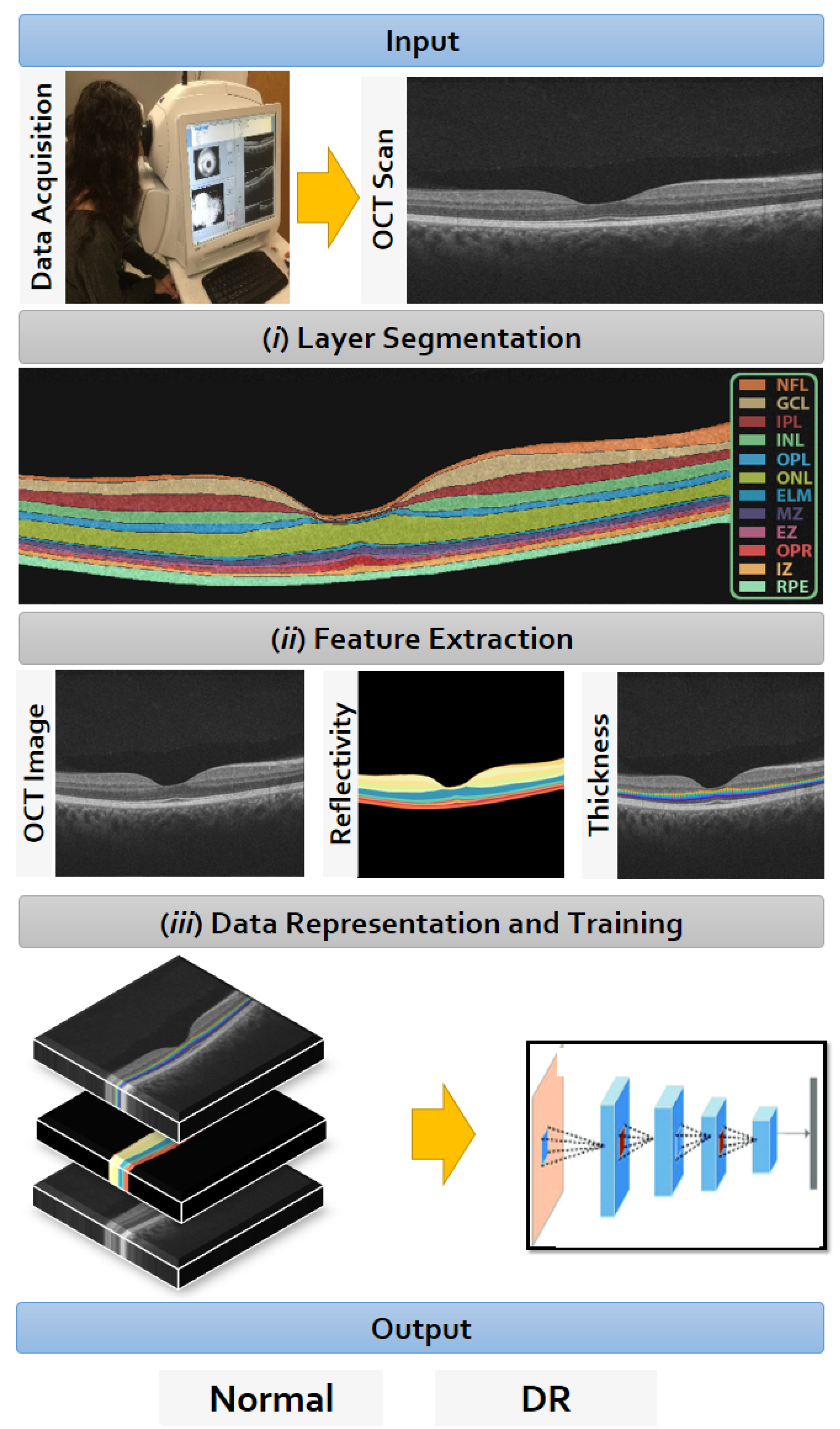
2. Materials and Methods
2.1. Data Collection
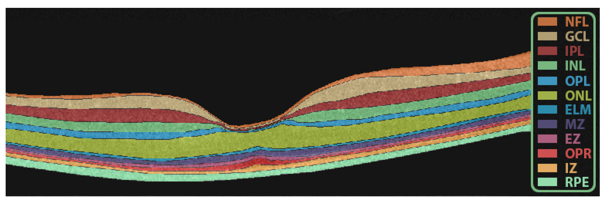
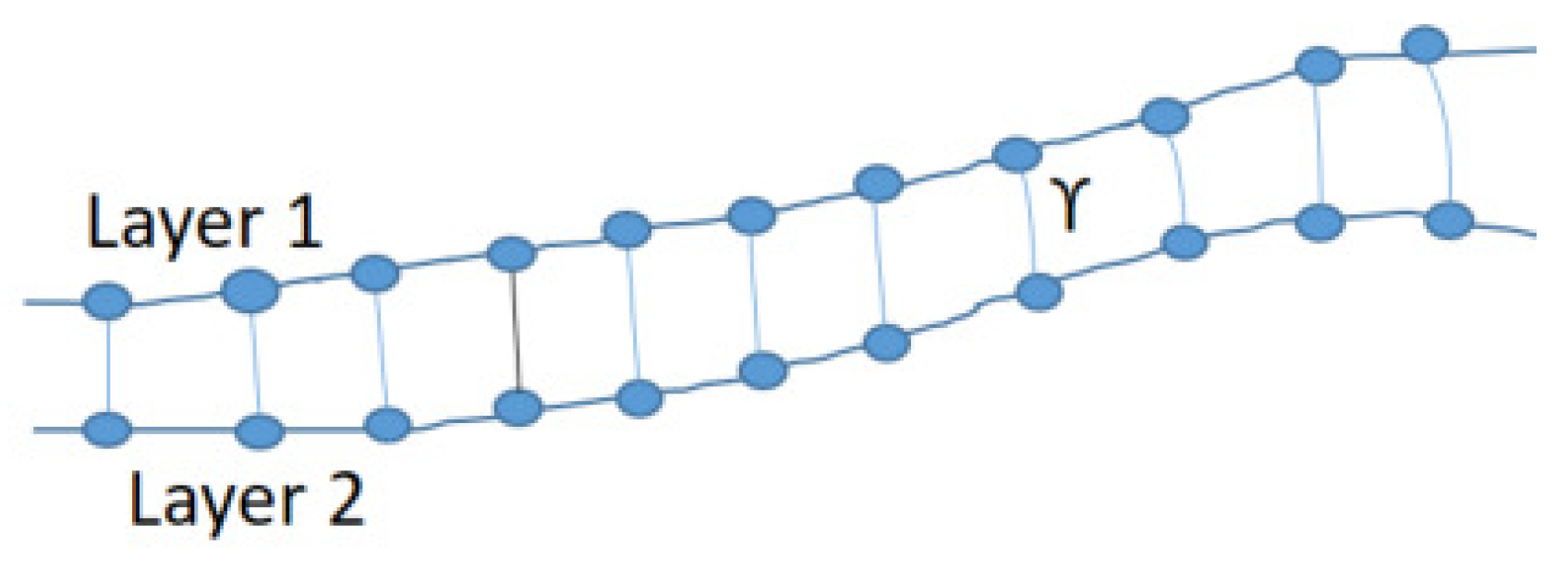
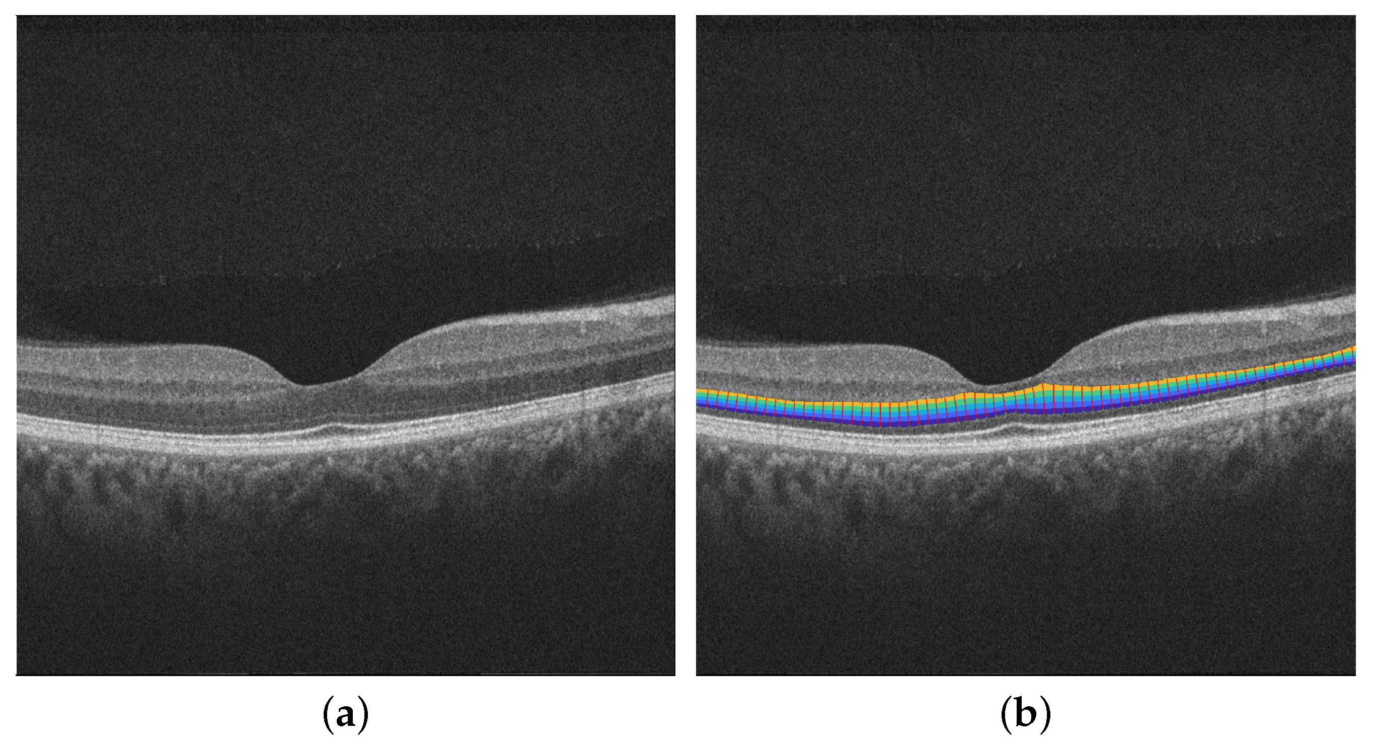
2.2. Retinal Layers Segmentation
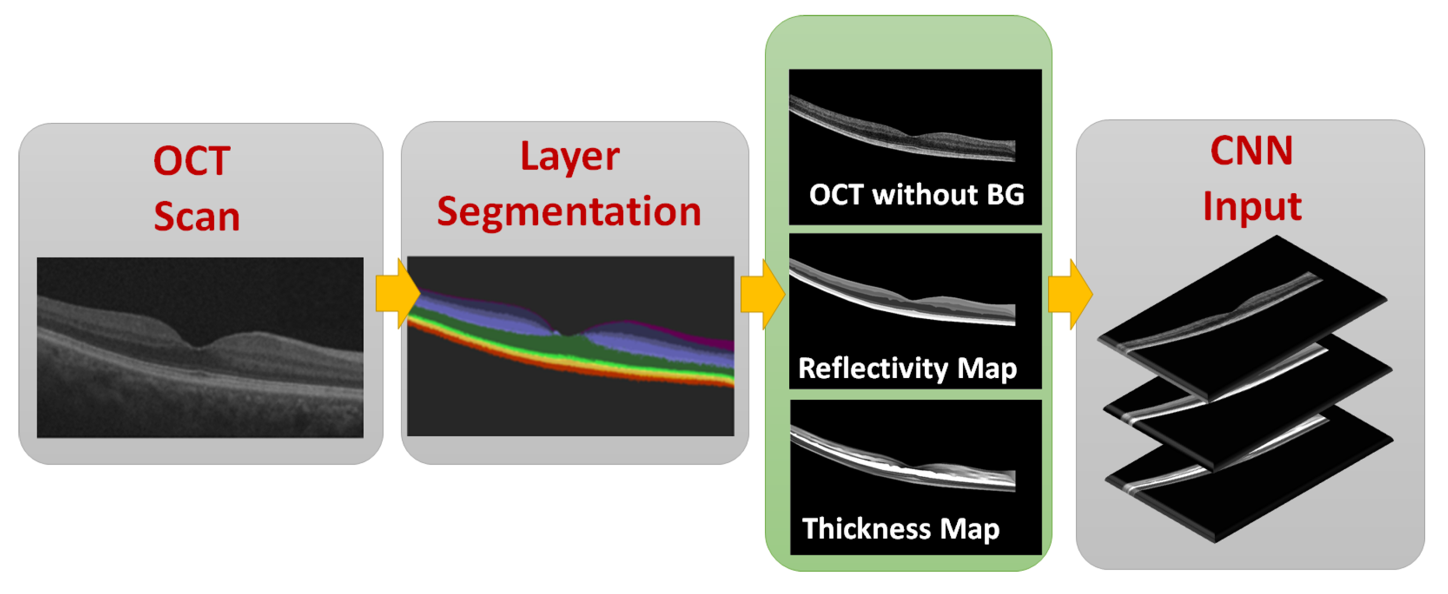
2.3. CNN Input Data Representation
2.3.1. OCT without BG
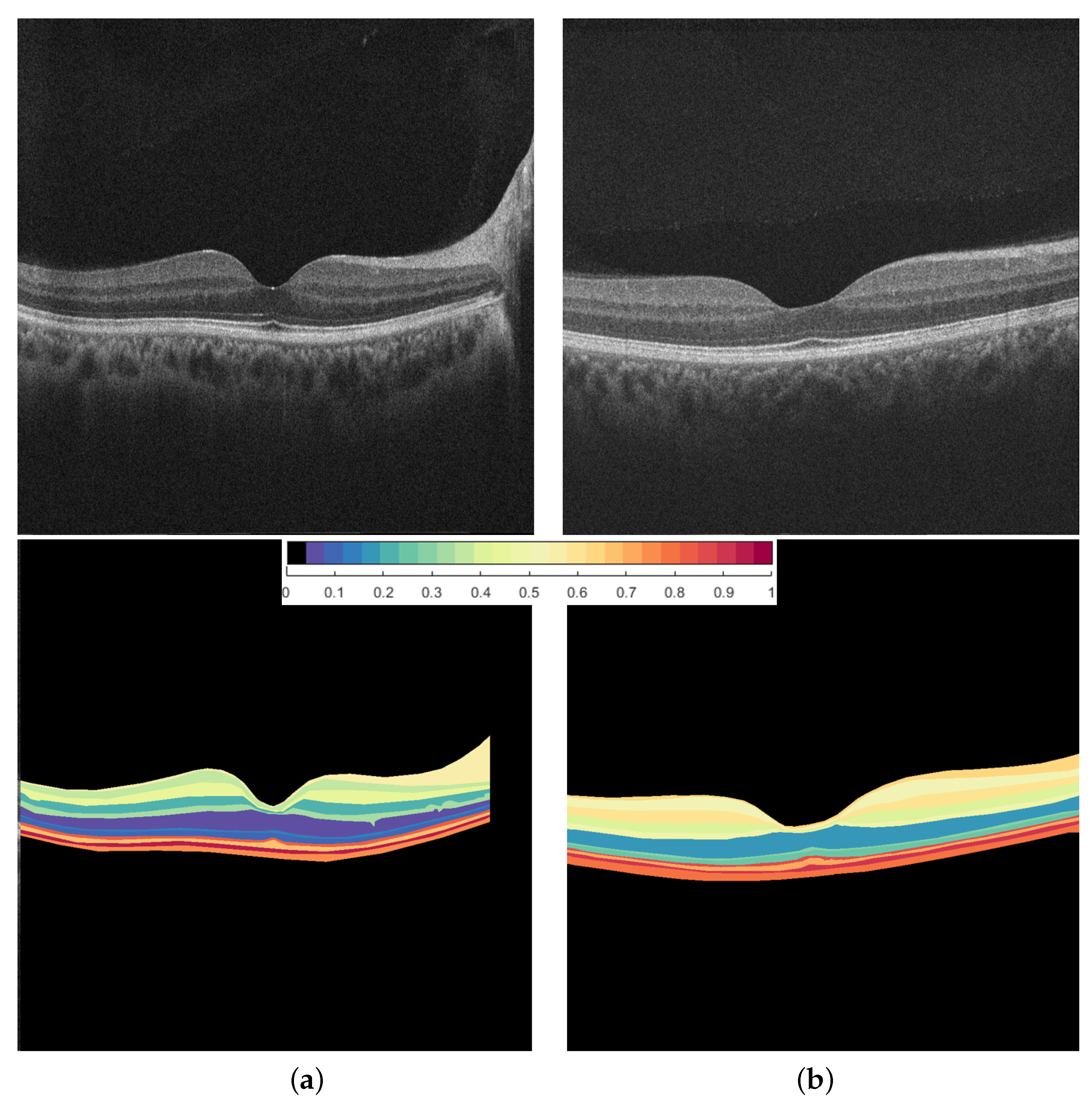
2.3.2. Reflectivity Map
2.3.3. Thickness Map
2.4. Data Representation to the CNN
2.5. Diagnostic CNN
- First convolutional layer with input of 256 × 256 and 16 kernels;
- Max. pooling layer;
- Second convolutional layer with 32 kernels;
- Max. pooling layer;
- Third convolutional layer with 64 kernels;
- Max. pooling layer;
- Fourth convolutional layer with 128 kernels;
- Max. pooling layer;
- The output of the last layer is then flattened and applied to the fully connected NN input;
- First layer of a fully connected dense layer of 4096 nodes with ReLu activation function;
- Second dense layer of 1024 nodes with ReLu activation function;
- Final single node with sigmoid activation to discriminate the two classes.
3. Results
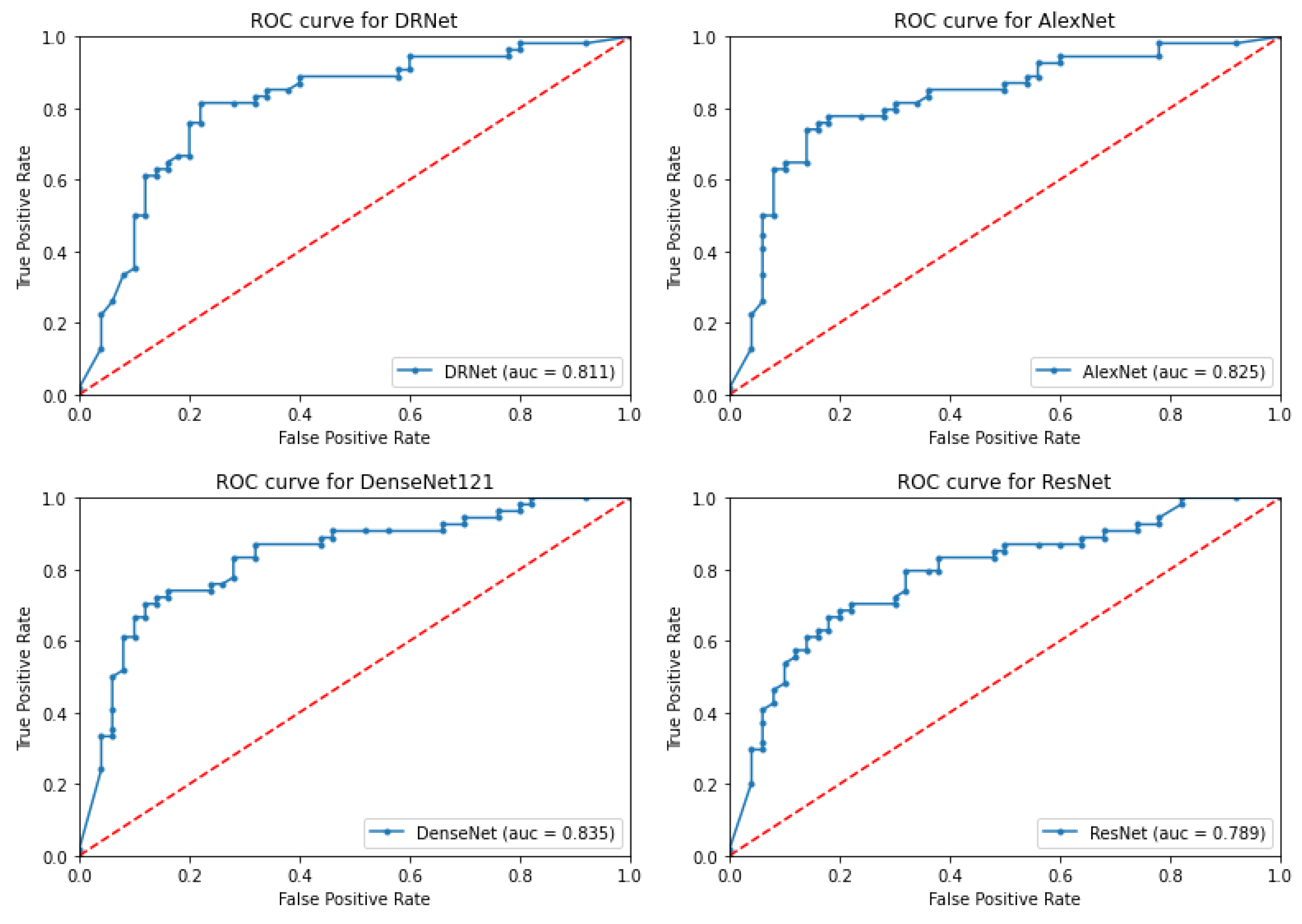
3.1. Proposed System Results
3.2. Ablation Study
4. Discussion
5. Conclusions
Author Contributions
Funding
Institutional Review Board Statement
Informed Consent Statement
Data Availability Statement
Conflicts of Interest
References
- Qiao, L.; Zhu, Y.; Zhou, H. Diabetic retinopathy detection using prognosis of microaneurysm and early diagnosis system for non-proliferative diabetic retinopathy based on deep learning algorithms. IEEE Access 2020, 8, 104292–104302. [Google Scholar] [CrossRef]
- Sabanayagam, C.; Banu, R.; Chee, M.L.; Lee, R.; Wang, Y.X.; Tan, G.; Jonas, J.B.; Lamoureux, E.L.; Cheng, C.Y.; Klein, B.E.; et al. Incidence and progression of diabetic retinopathy: A systematic review. Lancet Diabetes Endocrinol. 2019, 7, 140–149. [Google Scholar] [CrossRef]
- Mookiah, M.R.K.; Acharya, U.R.; Chua, C.K.; Lim, C.M.; Ng, E.Y.K.; Laude, A. Computer-aided diagnosis of diabetic retinopathy: A review. Comput. Biol. Med. 2013, 43, 2136–2155. [Google Scholar] [CrossRef]
- Bhardwaj, C.; Jain, S.; Sood, M. Hierarchical severity grade classification of non-proliferative diabetic retinopathy. J. Ambient. Intell. Humaniz. Comput. 2021, 12, 2649–2670. [Google Scholar] [CrossRef]
- Simonyan, K.; Zisserman, A. Very deep convolutional networks for large-scale image recognition. arXiv 2014, arXiv:1409.1556. [Google Scholar]
- He, K.; Zhang, X.; Ren, S.; Sun, J. Deep residual learning for image recognition. In Proceedings of the IEEE Conference on Computer Vision and Pattern Recognition, Las Vegas, NV, USA, 27–30 June 2016; pp. 770–778. [Google Scholar]
- Wang, S.; Wang, X.; Hu, Y.; Shen, Y.; Yang, Z.; Gan, M.; Lei, B. Diabetic retinopathy diagnosis using multichannel generative adversarial network with semisupervision. IEEE Trans. Autom. Sci. Eng. 2020, 18, 574–585. [Google Scholar] [CrossRef]
- Gadekallu, T.R.; Khare, N.; Bhattacharya, S.; Singh, S.; Maddikunta, P.K.R.; Srivastava, G. Deep neural networks to predict diabetic retinopathy. J. Ambient. Intell. Humaniz. Comput. 2020. [Google Scholar] [CrossRef]
- Kang, Y.; Fang, Y.; Lai, X. Automatic detection of diabetic retinopathy with statistical method and Bayesian classifier. J. Med. Imaging Health Inform. 2020, 10, 1225–1233. [Google Scholar] [CrossRef]
- Oh, K.; Kang, H.M.; Leem, D.; Lee, H.; Seo, K.Y.; Yoon, S. Early detection of diabetic retinopathy based on deep learning and ultra-wide-field fundus images. Sci. Rep. 2021, 11, 1897. [Google Scholar] [CrossRef]
- Stolte, S.; Fang, R. A survey on medical image analysis in diabetic retinopathy. Med. Image Anal. 2020, 64, 101742. [Google Scholar] [CrossRef]
- Akram, M.U.; Khalid, S.; Tariq, A.; Khan, S.A.; Azam, F. Detection and classification of retinal lesions for grading of diabetic retinopathy. Comput. Biol. Med. 2014, 45, 161–171. [Google Scholar] [CrossRef] [PubMed]
- Wan, S.; Liang, Y.; Zhang, Y. Deep convolutional neural networks for diabetic retinopathy detection by image classification. Comput. Electr. Eng. 2018, 72, 274–282. [Google Scholar] [CrossRef]
- Shankar, K.; Sait, A.R.W.; Gupta, D.; Lakshmanaprabu, S.K.; Khanna, A.; Pandey, H.M. Automated detection and classification of fundus diabetic retinopathy images using synergic deep learning model. Pattern Recognit. Lett. 2020, 133, 210–216. [Google Scholar] [CrossRef]
- Zhang, W.; Zhong, J.; Yang, S.; Gao, Z.; Hu, J.; Chen, Y.; Yi, Z. Automated identification and grading system of diabetic retinopathy using deep neural networks. Knowl. Based Syst. 2019, 175, 12–25. [Google Scholar] [CrossRef]
- Pratt, H.; Coenen, F.; Broadbent, D.M.; Harding, S.P.; Zheng, Y. Convolutional neural networks for diabetic retinopathy. Procedia Comput. Sci. 2016, 90, 200–205. [Google Scholar] [CrossRef] [Green Version]
- Gao, Z.; Li, J.; Guo, J.; Chen, Y.; Yi, Z.; Zhong, J. Diagnosis of diabetic retinopathy using deep neural networks. IEEE Access 2018, 7, 3360–3370. [Google Scholar] [CrossRef]
- Sayres, R.; Taly, A.; Rahimy, E.; Blumer, K.; Coz, D.; Hammel, N.; Krause, J.; Narayanaswamy, A.; Rastegar, Z.; Wu, D.; et al. Using a deep learning algorithm and integrated gradients explanation to assist grading for diabetic retinopathy. Ophthalmology 2019, 126, 552–564. [Google Scholar] [CrossRef] [Green Version]
- Zhao, Z.; Zhang, K.; Hao, X.; Tian, J.; Chua, M.C.H.; Chen, L.; Xu, X. Bira-net: Bilinear attention net for diabetic retinopathy grading. In Proceedings of the 2019 IEEE International Conference on Image Processing (ICIP), Taipei, Taiwan, 22–25 September 2019; IEEE: Piscataway, NJ, USA, 2019; pp. 1385–1389. [Google Scholar]
- Li, X.; Hu, X.; Yu, L.; Zhu, L.; Fu, C.W.; Heng, P.A. CANet: Cross-disease attention network for joint diabetic retinopathy and diabetic macular edema grading. IEEE Trans. Med. Imaging 2020, 39, 1483–1493. [Google Scholar] [CrossRef] [Green Version]
- Gulshan, V.; Rajan, R.P.; Widner, K.; Wu, D.; Wubbels, P.; Rhodes, T.; Whitehouse, K.; Coram, M.; Corrado, G.; Ramasamy, K.; et al. Performance of a deep-learning algorithm vs manual grading for detecting diabetic retinopathy in India. JAMA Ophthalmol. 2019, 137, 987–993. [Google Scholar] [CrossRef] [Green Version]
- Sandhu, H.S.; Eltanboly, A.; Shalaby, A.; Keynton, R.S.; Schaal, S.; El-Baz, A. Automated diagnosis and grading of diabetic retinopathy using optical coherence tomography. Investig. Ophthalmol. Vis. Sci. 2018, 59, 3155–3160. [Google Scholar] [CrossRef] [Green Version]
- Li, X.; Shen, L.; Shen, M.; Tan, F.; Qiu, C.S. Deep learning based early stage diabetic retinopathy detection using optical coherence tomography. Neurocomputing 2019, 369, 134–144. [Google Scholar] [CrossRef]
- ElTanboly, A.; Ismail, M.; Shalaby, A.; Switala, A.; El-Baz, A.; Schaal, S.; Gimel’farb, G.; El-Azab, M. A computer-aided diagnostic system for detecting diabetic retinopathy in optical coherence tomography images. Med. Phys. 2017, 44, 914–923. [Google Scholar] [CrossRef] [PubMed]
- Sandhu, H.S.; Eladawi, N.; Elmogy, M.; Keynton, R.; Helmy, O.; Schaal, S.; El-Baz, A. Automated diabetic retinopathy detection using optical coherence tomography angiography: A pilot study. Br. J. Ophthalmol. 2018, 102, 1564–1569. [Google Scholar] [CrossRef] [PubMed]
- Sandhu, H.S.; Elmogy, M.; Sharafeldeen, A.T.; Elsharkawy, M.; El-Adawy, N.; Eltanboly, A.; Shalaby, A.; Keynton, R.; El-Baz, A. Automated diagnosis of diabetic retinopathy using clinical biomarkers, optical coherence tomography, and optical coherence tomography angiography. Am. J. Ophthalmol. 2020, 216, 201–206. [Google Scholar] [CrossRef]
- Alam, M.; Zhang, Y.; Lim, J.I.; Chan, R.V.; Yang, M.; Yao, X. Quantitative optical coherence tomography angiography features for objective classification and staging of diabetic retinopathy. Retina 2020, 40, 322–332. [Google Scholar] [CrossRef]
- ElTanboly, A.H.; Palacio, A.; Shalaby, A.M.; Switala, A.E.; Helmy, O.; Schaal, S.; El-Baz, A. An automated approach for early detection of diabetic retinopathy using SD-OCT images. Front. Biosci. 2018, 10, 197–207. [Google Scholar]
- Schaal, S.; Ismail, M.; Palacio, A.C.; ElTanboly, A.; Switala, A.; Soliman, A.; Neyer, T.; Hajrasouliha, A.; Hadayer, A.; Sigford, D.K.; et al. Subtle early changes in diabetic retinas revealed by a novel method that automatically quantifies spectral domain optical coherence tomography (SD-OCT) images. Investig. Ophthalmol. Vis. Sci. 2016, 57, 6324. [Google Scholar]
- Krizhevsky, A.; Sutskever, I.; Hinton, G.E. Imagenet classification with deep convolutional neural networks. Adv. Neural Inf. Process. Syst. 2012, 25, 1106–1114. [Google Scholar] [CrossRef]
- Huang, G.; Liu, Z.; Van Der Maaten, L.; Weinberger, K.Q. Densely connected convolutional networks. In Proceedings of the IEEE Conference on Computer Vision and Pattern Recognition, Honolulu, HI, USA, 21–26 July 2017; pp. 4700–4708. [Google Scholar]
- Szegedy, C.; Sergey, I.; Vincent, V.; Alemi, A.A. Inception-v4, inception-resnet and the impact of residual connections on learning. In Proceedings of the Thirty-First AAAI Conference on Artificial Intelligence, San Francisco, CA, USA, 4–9 February 2017. [Google Scholar]
- Deng, J.; Dong, W.; Socher, R.; Li, L.J.; Li, K.; Li, F.-F. Imagenet: A large-scale hierarchical image database. In Proceedings of the IEEE Conference on Computer Vision and Pattern Recognition, Miami, FL, USA, 20–25 June 2009; pp. 248–255. [Google Scholar]
- Hagras, H. Toward human-understandable, explainable AI. Computer 2018, 51, 28–36. [Google Scholar] [CrossRef]


| Used | Gray | Gray | Gray | Fused | Fused | Fused |
|---|---|---|---|---|---|---|
| Network | Acc | Sen | Sp | Acc | Sen | Sp |
| DRNet | 76.3 ± 1.4 | 76.0 ± 1.0 | 77.7 ± 0.9 | 93.3 ± 1.4 | 92.5 ± 0.6 | 94.0 ± 0.9 |
| AlexNet | 73.8 ± 8 | 72.0 ± 5 | 75.9 ± 2.7 | 93.5 ± 2 | 93.1 ± 1.2 | 93.5 ± 0.6 |
| DenseNet121 | 89.8 ± 3 | 86.1 ± 3 | 92.4 ± 2.2 | 94.8 ± 2 | 96.0 ± 5 | 94.5 ± 0.7 |
| ResNet101 | 82.8 ± 6 | 82.1 ± 5 | 86.2 ± 4.7 | 88.5 ± 2 | 85.0 ± 5 | 91.2 ± 4.7 |
| Used | Gray | Gray | Gray | Fused | Fused | Fused |
|---|---|---|---|---|---|---|
| Network | Acc | Sen | Sp | Acc | Sen | Sp |
| DRNet | 85.3 ± 5 | 83.1 ± 1.1 | 86.6 ± 0.9 | 97.1 ± 0.7 | 98.0 ± 0.4 | 96.7 ± 0.5 |
| AlexNet | 86.1 ± 3 | 84.0 ± 2.9 | 89.0 ± 3.5 | 97.7 ± 0.5 | 98.1 ± 0.6 | 98.3 ± 0.5 |
| DenseNet121 | 90.1 ± 2 | 87.8 ± 2 | 93.1 ± 2.4 | 97.3 ± 0.4 | 98.3 ± 0.5 | 98.0 ± 0.4 |
| ResNet101 | 83.2 ± 3 | 84.3 ± 4.1 | 86.1 ± 3.7 | 91.6 ± 2.8 | 92.3 ± 2.1 | 91.1 ± 1.8 |
| Applied Network | Acc% | Sen% | Sp% |
|---|---|---|---|
| DRNet | 88.1 ± 1.5 | 84.0 ± 2.2 | 90.0 ± 1.7 |
| AlexNet | 89.5 ± 2.8 | 86.1 ± 2.5 | 92.1 ± 2.7 |
| DenseNet121 | 89.3 ± 3 | 86.2 ± 1.6 | 92.5 ± 1.8 |
| ResNet101 | 82.2 ± 6 | 80.3 ± 3.1 | 85.0 ± 2.9 |
| Applied Network | Acc% | Sen% | Sp% |
|---|---|---|---|
| DRNet | 89.9 ± 0.8 | 86.0 ± 2.2 | 92.6.1 ± 2.0 |
| AlexNet | 91.8 ± 1.4 | 89.0 ± 2.9 | 94.5 ± 2.1 |
| DenseNet121 | 91.3 ± 2 | 88.0 ± 1.8 | 94.4 ± 2.3 |
| ResNet101 | 84.1 ± 5 | 82.3 ± 4 | 85.1 ± 3.1 |
Publisher’s Note: MDPI stays neutral with regard to jurisdictional claims in published maps and institutional affiliations. |
© 2022 by the authors. Licensee MDPI, Basel, Switzerland. This article is an open access article distributed under the terms and conditions of the Creative Commons Attribution (CC BY) license (https://creativecommons.org/licenses/by/4.0/).
Share and Cite
Haggag, S.; Elnakib, A.; Sharafeldeen, A.; Elsharkawy, M.; Khalifa, F.; Farag, R.K.; Mohamed, M.A.; Sandhu, H.S.; Mansoor, W.; Sewelam, A.; et al. A Computer-Aided Diagnostic System for Diabetic Retinopathy Based on Local and Global Extracted Features. Appl. Sci. 2022, 12, 8326. https://doi.org/10.3390/app12168326
Haggag S, Elnakib A, Sharafeldeen A, Elsharkawy M, Khalifa F, Farag RK, Mohamed MA, Sandhu HS, Mansoor W, Sewelam A, et al. A Computer-Aided Diagnostic System for Diabetic Retinopathy Based on Local and Global Extracted Features. Applied Sciences. 2022; 12(16):8326. https://doi.org/10.3390/app12168326
Chicago/Turabian StyleHaggag, Sayed, Ahmed Elnakib, Ahmed Sharafeldeen, Mohamed Elsharkawy, Fahmi Khalifa, Rania Kamel Farag, Mohamed A. Mohamed, Harpal Singh Sandhu, Wathiq Mansoor, Ashraf Sewelam, and et al. 2022. "A Computer-Aided Diagnostic System for Diabetic Retinopathy Based on Local and Global Extracted Features" Applied Sciences 12, no. 16: 8326. https://doi.org/10.3390/app12168326
APA StyleHaggag, S., Elnakib, A., Sharafeldeen, A., Elsharkawy, M., Khalifa, F., Farag, R. K., Mohamed, M. A., Sandhu, H. S., Mansoor, W., Sewelam, A., & El-Baz, A. (2022). A Computer-Aided Diagnostic System for Diabetic Retinopathy Based on Local and Global Extracted Features. Applied Sciences, 12(16), 8326. https://doi.org/10.3390/app12168326