A Fast and Simple Method for Absolute Orientation Estimation Using a Single Vanishing Point

Abstract

Absolute orientation estimation is one of the key steps in computer vision, and n 2D–3D point correspondences can be used to obtain the absolute orientation, which is known as the perspective-n-point problem (PnP). The lowest number of point correspondences is three if there is no other information, and the corresponding algorithm is called the P3P solver. In practice, the real scene may consist of some geometric information, e.g., the vanishing point. When scenes contain parallel lines, they intersect at vanishing points. Hence, to reduce the number of point correspondences and increase the computational speed, we proposed a fast and simple method for absolute orientation estimation using a single vanishing point. First, the inertial measurement unit (IMU) was used to obtain the rotation of the camera around the Y-axis (i.e., roll angle), which could simplify the orientation estimation. Then, one vanishing point was used to estimate the coarse orientation because it contained direction information in both the camera frame and world frame. Finally, our proposed method used a non-linear optimization algorithm for solution refining. The experimental results show that compared with several state-of-the-art orientation estimation solvers, our proposed method had a better performance regarding numerical stability, noise sensitivity, and computational speed in synthetic data and real images.

1. Introduction

Orientation estimation for cameras is an old but continually developing subject, and the oldest paper on this topic was published in 1841 [1], which described a PnP (perspective-n-point) problem where n 2D–3D point correspondences between 3D points of known positions and their 2D image projections were used to estimate the camera orientation and position. Recently, a large number of PnP solvers have been published [2,3,4,5,6,7] and have expand the orientation estimation methods. The reason this topic is still popular is that pose estimation is essential in computer vision [8,9,10,11] and 3D reconstruction [12,13,14,15]. In addition, some solvers use 2D–3D line correspondences, not point correspondences, to estimate the camera orientation, which are known as PnL (perspective-n-line) solvers [16,17,18]. For both 2D–3D point and line correspondences, each correspondence provides two constraints [19], and because the camera pose has six dof (three for orientation and three for position), the minimal number of correspondences is three. What is more, the six dof are coupled and cannot be estimated independently if there is no other constraint.

With the recent development of sensors, orientation sensors, e.g., IMU or gradienter, have been widely used and the accuracy of the cheap IMU is increasing [20]. This popularity has resulted in more and more cameras being equipped with orientation sensors in computer vision and SfM [21,22], which can simplify the problem of pose estimation. It also inspired the idea to propose a new and fast method in this paper.

For PnP solvers, for 2D–3D point correspondences of known positions not fewer than three, many algorithms have been proposed [23,24,25]. Note that most algorithms cannot estimate the orientation or position independently, and hence the number of point correspondences cannot be decreased. When the number of 2D–3D point correspondences is three, up to four solutions can be given through the non-linear algorithm, and the corresponding methods are called P3P solvers [26,27,28,29]. When more 2D–3D point correspondences are given, some intrinsic camera parameters can be simultaneously estimated, i.e., using P4Pf solvers [30,31] and P5Pfr solvers [32]. When the number of 2D–3D point correspondences of known positions is not fewer than six, the camera orientation and position can be estimated linearly, and the corresponding solvers are called DLTs (direct linear transforms) [33,34,35,36].

In practice, however, it is difficult to obtain 3D points with known positions. Some algorithms have been proposed to reduce the number of 3D points with known positions or orientations [37,38,39], but they still need two or more 3D points. In some scenes, 3D lines exist (e.g., ceilings and floors indoor, or the walls of buildings) and thus many PnL solvers have been proposed [40,41,42,43] that can use this information. Similar to the 3D points in the PnP problem, 3D lines with known absolute positions are also difficult to obtain. This restriction prevents the application of PnL solvers from scenarios where not enough 3D lines with known absolute positions are provided. However, when scenes contain parallel lines, they intersect at a vanishing point in images, and some algorithms [44,45,46,47] use this information to estimate the camera pose because many parallel lines, e.g., ceilings and floors indoors, may exist in certain scenarios. Grammatikopoulos proposed a method to use two vanishing points to estimate the camera pose [48]. However, this method has a disadvantage as it supposes that the parallel lines of the first set are perpendicular to those of the second, and the intersection of the two sets is the origin of the world frame. When more vanishing points or other constraints are given, the disadvantage can be overcome and more parameters of the camera can be estimated [49]. More vanishing points can estimate more parameters and improve the accuracy. However, many scenarios may only have one or two vanishing points and thus the origin of the world frame could be arbitrary, which limits the corresponding methods from being employed.

In this paper, we proposed a fast and simple method for absolute orientation estimation using a single vanishing point to overcome these disadvantages descried above. Our proposed method uses IMU to provide the roll angle, and then estimates the camera orientation using only one vanishing point. Moreover, the positions of the parallel 3D lines of this vanishing point are not essential, only the direction vector. Our proposed method can separate the camera orientation from the position, and hence the orientation can be estimated independently because the six dof are not coupled in our method. This increases the computational speed. The angular accuracy of the roll angle in low cost IMUs [39,50] is about 0.02°, and hence using the roll information cannot decrease the accuracy of our proposed method. The known roll angle can simplify the rotation matrix, and this simplification results in being able to estimate the other two orientations independently, which also enormously improve both the efficiency and accuracy, because the system of non-linear equations could decrease both. Then, our proposed method uses a vanishing point of parallel lines whose direction vector is known in order to estimate the camera orientation. Actually, the vanishing point contains the rotation between the camera frame and world frame, and it does not contain the information about the translation; thus, the coarse orientation can be estimated independently. Last, a non-linear optimization algorithm is given to refine the orientation and it improves the accuracy of our proposed method. In addition, the usable range of our proposed method is given, which is the vanishing point that cannot be used to estimate orientation in this method, and the algebraic derivation is given.

The rest of this paper is organized as follows: Section 2 provides the Materials and Methods, including the vanishing point and method statement, orientation refining, and limitations of parallel lines and their algebraic derivations. Section 3 is the Experiments and Results, including the numerical stability, noise sensitivity, computational speed in synthetic data, and testing in real images, compared with several state-of-the-art orientation estimation solvers. Section 4 provides the Discussion and Section 5 is the Conclusions.

2. Materials and Methods

In this paper, the roll angle was set to zero using the IMU mounted on the camera. Then, a single vanishing point was used to estimate the orientation. Here, the standard pinhole camera model [51] was used and we assumed its principal point was the center of the image, and the focal length was given by the image header (EXIF). We systematically formulated this problem in the following basic procedures.

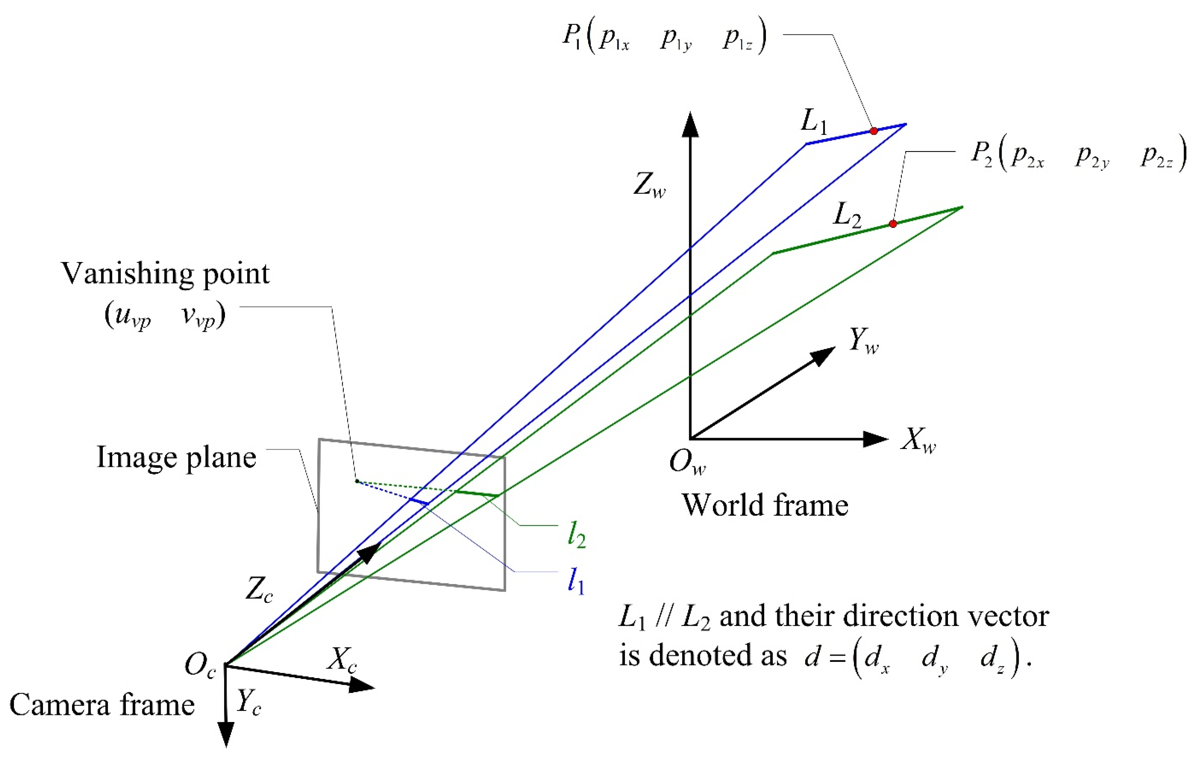
2.1. Vanishing Point and Method Statement

The geometrical drawing of this paper is illustrated in Figure 1. The direction vector of a 3D line L₁ in the camera frame Oc_XcYcZc is denoted as $d=\left(\begin{array}{ccc}{d}_x& d_y& d_z\end{array}\right)$ and a point $P_1\left(\begin{array}{ccc}{p}_{1x}& p_{1y}& p_{1z}\end{array}\right)$ is on this line.

From Figure 1, the 3D line L₁ can be written as follows:

$$L_1=P_1+k_1\cdot d$$

(1)

Here, k₁ is the arbitrary scale value. Similarly, another 3D line L₂ that is parallel to, L₁, in the camera frame can be denoted as $L_2=P_2+k_2\cdot d$. k₂ is an arbitrary scale value and $P_2\left(\begin{array}{ccc}{p}_{2x}& p_{2y}& p_{2z}\end{array}\right)$ is a 3D point on line L₂. According to the standard pinhole camera model, the image projection l₁ of the 3D line L₁ can be written as follows:

$$\begin{array}{l}{u}_1=f\frac{X_c}{Z_c}=f\frac{p_{1x}+k_1\cdot d_x}{p_{1z}+k_1\cdot d_z}\\ v_1=f\frac{Y_c}{Z_c}=f\frac{p_{1y}+k_1\cdot d_y}{p_{1z}+k_1\cdot d_z}\end{array}$$

(2)

Here, f is the focal length, which can be either known or unknown in this paper. When $k_1\to \infty$ and d_z is not zero, the image projection of line L₁ can be denoted as follows:

$$\begin{array}{l}{u}_{1\infty }=\underset{k_1\to \infty }{\lim }f\frac{p_{1x}+k_1\cdot d_x}{p_{1z}+k_1\cdot d_z}=\frac{d_x}{d_z}\\ v_{1\infty }=\underset{k_1\to \infty }{\lim }f\frac{p_{1y}+k_1\cdot d_y}{p_{1z}+k_1\cdot d_z}=\frac{d_y}{d_z}\end{array}$$

(3)

Similarly, the image projection l₂ of line L₂ can be denoted as follows:

$$\begin{array}{l}{u}_{2\infty }=\underset{k_2\to \infty }{\lim }f\frac{p_{2x}+k_2\cdot d_x}{p_{2z}+k_2\cdot d_z}=\frac{d_x}{d_z}\\ v_{2\infty }=\underset{k_2\to \infty }{\lim }f\frac{p_{2y}+k_2\cdot d_y}{p_{2z}+k_2\cdot d_z}=\frac{d_y}{d_z}\end{array}$$

(4)

It can be seen that the image projections of the 3D line L₁, L₂, in camera frame intersects at the same point, which is called the vanishing point.

$$\begin{array}{l}{u}_{vp}=\frac{d_x}{d_z}\\ v_{vp}=\frac{d_y}{d_z}\end{array}$$

(5)

The image projections of l₁ and l₂ can be extracted and thus the corresponding vanishing point $\left(\begin{array}{cc}{u}_{vp}& v_{vp}\end{array}\right)$ is known. Consequently, the direction vector of the parallel lines of L₁ and L₂ can be found from Equation (5) using

$$d=\left(\begin{array}{ccc}{d}_x& d_y& d_z\end{array}\right)=d_z\cdot \left(\begin{array}{ccc}{u}_{vp}& v_{vp}& 1\end{array}\right)$$

(6)

Hence, the unit direction vector d_c of the parallel lines of L₁ and L₂ in the camera frame is obtained using

$$d_c=\left(\begin{array}{ccc}{d}_{cx}& d_{cy}& d_{cz}\end{array}\right)=\frac{1}{\sqrt{u_{vp}^2+v_{vp}^2+1}}\left(\begin{array}{ccc}{u}_{vp}& v_{vp}& 1\end{array}\right)$$

(7)

It can be seen that the unit direction vector of the parallel lines in the camera frame can be obtained through the corresponding vanishing point. Then, the unit direction vector d_w of the parallel lines of L₁ and L₂ in the world frame can be given according the rotation between the world frame and the camera frame, as follows.

$$d_w=\left[\begin{array}{c}{d}_{wx}\\ d_{wy}\\ d_{wz}\end{array}\right]=R_{c\_w}\cdot \left[\begin{array}{c}{d}_{cx}\\ d_{cy}\\ d_{cz}\end{array}\right]$$

(8)

Here, $R_{c\_w}$ is the rotation matrix that contains the information of three rotational angles $\left(\begin{array}{ccc}{a}_x& a_y& a_z\end{array}\right)$. Because the roll angle is set to zero through the IMU, $a_y=0$ and the other two roatational angles are unknown and need to be estimated in this paper. Then, according to the rigid motion, $R_{c\_w}$ can be written as

$$R_{c\_w}=\left[\begin{array}{ccc}\cos a_z& -\sin a_z\cdot \cos a_x& \sin a_z\sin a_x\\ \sin a_z& \cos a_z\cos a_x& -\cos a_z\sin a_x\\ 0& \sin a_x& \cos a_x\end{array}\right]$$

(9)

When the unit direction vector d_w of the parallel lines of L₁ and L₂ in the world frame is known, from the vanishing point and Formulas (8) and (9), three equations can be given and the third equation is written as follows.

$$d_{cy}\cdot \sin a_x+d_{cz}\cdot \cos a_x=d_{wz}$$

(10)

Then, the rotational angle $a_x$ is obtained using

$$a_x=a_1-a_2,\{\begin{array}{c}{a}_1=\arcsin \frac{d_{wz}}{\sqrt{d_{cy}^2+d_{cz}^2}}\\ a_2=\arcsin \frac{d_{cz}}{\sqrt{d_{cy}^2+d_{cz}^2}}\end{array}$$

(11)

Last, the rotational angle $a_z$ can be estimated according to $a_x$ and formulas (8) and (9), as follows.

$$a_z=a_3-a_4,\{\begin{array}{c}{a}_3=\arcsin \frac{d_{wx}}{\sqrt{d_{cx}^2+{\left(d_{cz}\cdot \sin a_x-d_{cy}\cdot \cos a_x\right)}^2}}\\ a_2=\arcsin \frac{d_{cx}}{\sqrt{d_{cx}^2+{\left(d_{cz}\cdot \sin a_x-d_{cy}\cdot \cos a_x\right)}^2}}\end{array}$$

(12)

Now, the coarse camera orientation is obtained.

2.2. Orientation Refining

In this section, the coarse camera orientation $\left(\begin{array}{cc}{a}_x& a_z\end{array}\right)$ obtained in Section 2.1 is used as the initial solution $\left(\begin{array}{cc}{a}_{x0}& a_{z0}\end{array}\right)$ to refine the camera orientation. Three cost functions can be found, from Equations (8) and (9), as follows.

$$\begin{array}{l}{f}_1=\cos a_z\cdot d_{cx}-\sin a_z\cdot \cos a_x\cdot d_{cy}+\sin a_z\cdot \sin a_x\cdot d_{cz}-d_{wx}\\ f_2=\sin a_z\cdot d_{cx}+\cos a_z\cdot \cos a_x\cdot d_{cy}-\cos a_z\cdot \sin a_x\cdot d_{cz}-d_{wy}\\ f_3=0\cdot d_{cx}+\sin a_x\cdot d_{cy}+\cos a_x\cdot d_{cz}-d_{wz}\end{array}$$

(13)

The goal of orientation refining is to minimize $f_i\left(i=1,2,3\right)$ with the initial solution $\left(\begin{array}{cc}{a}_{x0}& a_{z0}\end{array}\right)$. Here, the Gauss–Newton method [52] was used and the processing was as follows.

First, according to the cost functions (Equation (13)), the Jacobian matrix J is given by

$$J^T=\left[\begin{array}{ccc}\frac{\partial f_1}{\partial a_x}& \frac{\partial f_2}{\partial a_x}& \frac{\partial f_3}{\partial a_x}\\ \frac{\partial f_1}{\partial a_z}& \frac{\partial f_2}{\partial a_z}& \frac{\partial f_3}{\partial a_z}\end{array}\right]$$

(14)

Then, we refine the orientation using

$$\left[\begin{array}{c}{a}_{xk+1}\\ a_{zk+1}\end{array}\right]=\left[\begin{array}{c}{a}_{xk}\\ a_{zk}\end{array}\right]-{\left(J^{T}J\right)}^{-1}{J}^T\left[\begin{array}{c}{f}_1\\ f_2\\ f_3\end{array}\right]$$

(15)

Here, $J^{T}J$ is the Hessian matrix. This is an iterative algorithm and a parameter will be given to stop the iteration

$$t=\sqrt{{\left(a_{xk+1}-a_{xk}\right)}^2+{\left(a_{zk+1}-a_{zk}\right)}^2}$$

(16)

If t is below the threshold we set, the iteration stops and the orientation refining is finished.

2.3. Limitation of Parallel Lines

In Section 2.1, only one vanishing point is used to estimate the camera orientation and this expands the range of application for our proposed method. However, the limitation of parallel lines exists in this paper. In this section, we assume this limitation, i.e., $d_w\ne \left(\begin{array}{ccc}0& 0& 1\end{array}\right)$ and its algebraic derivation is conducted as follows.

Here, we assume the unit direction vector d_w of the parallel lines of L₁ and L₂ in the world frame is $\left(\begin{array}{ccc}0& 0& 1\end{array}\right)$. From Formulas (8) and (9), we can obtain

$$\begin{gathered} \left[\begin{array}{c}{d}_{cx}\\ d_{cy}\\ d_{cz}\end{array}\right]=R_{\mathrm{w}\_\mathrm{c}}\cdot \left[\begin{array}{c}{d}_{wx}\\ d_{wy}\\ d_{wz}\end{array}\right]=R_{\mathrm{w}\_\mathrm{c}}\cdot \left[\begin{array}{c}0\\ 0\\ 1\end{array}\right] \\ {R}_{\mathrm{w}\_\mathrm{c}}=\left[\begin{array}{ccc}\cos a_z& \sin a_z& 0\\ -\cos a_x\sin a_z& \cos a_x\cos a_z& \sin a_x\\ \sin a_x\sin a_z& -\sin a_x\cos a_z& \cos a_x\end{array}\right] \end{gathered}$$

(17)

Consequently, the unit direction vector d_c in the camera frame can be given using

$$\begin{array}{l}{d}_{cx}=0\\ d_{cy}=\sin a_x\\ d_{cz}=\cos a_x\end{array}$$

(18)

From the first equation of formula (8), a new equation can be given

$$d_{cx}\cos a_z+\left(d_{cz}\sin a_x-d_{cy}\cos a_x\right)\sin a_z=0$$

(19)

Equation (19) is rewritten using formula (18), and a new equation is obtained

$$0\cdot \cos a_z+0\cdot \sin a_z=0$$

(20)

From Equation (20), it can be seen that $a_z$ can be an arbitrary value. This means there are infinite solutions of camera orientation and hence we cannot estimate the orientation if $d_w=\left(\begin{array}{ccc}0& 0& 1\end{array}\right)$.

After analyzing the limitation of our proposed method theoretically, we analyzed it using intuitional geometry. The projections of parallel lines of L₁ and L₂ whose direction vector is $\left(\begin{array}{ccc}0& 0& 1\end{array}\right)$ in world frame are illustrated in Figure 2.

In Figure 2, the initial world frame $O_{w1}-X_{w1}{Y}_{w1}{Z}_{w1}$ is rotated around the Z-axis by α degrees to the new world frame $O_{wn}-X_{wn}{Y}_{wn}{Z}_{wn}$. It can be seen that the direction vector of parallel lines of L₁ and L₂ is not changed, and is still $\left(\begin{array}{ccc}0& 0& 1\end{array}\right)$. Moreover, the spatial positions of the two lines in the camera frame $O_c-X_c{Y}_c{Z}_c$ are also not changed, which means their image projections of l₁ and l₂ are not changed after rotating. In brief, the 2D–3D line correspondences of parallel lines L₁ and L₂ are not changed when the world frame is rotated around the Z-axis, and hence the corresponding vanishing point is unchanged. Now, this vanishing point and the direction vector can be obtained from the camera frame $O_c-X_c{Y}_c{Z}_c$ and world frame $O_{w1}-X_{w1}{Y}_{w1}{Z}_{w1}$, respectively, but can also be obtained from the camera frame $O_c-X_c{Y}_c{Z}_c$ and world frame $O_{wn}-X_{wn}{Y}_{wn}{Z}_{wn}$, respectively. The phenomenon shows that infinite solutions can be estimated using parallel lines whose direction vector is $\left(\begin{array}{ccc}0& 0& 1\end{array}\right)$, and we cannot obtain the uniqueness. This is consistent with the results of the algebraic derivation above.

Hence, if $d_w=\left(\begin{array}{ccc}0& 0& 1\end{array}\right)$, we use another rotation order and the new rotation matrix is

$$R_{w\_c2}=\left[\begin{array}{ccc}\cos a_x& \sin a_x\cos a_z& \sin a_x\sin a_z\\ -\sin a_x& \cos a_x\cos a_z& \sin a_z\cos a_x\\ 0& -\sin a_z& \cos a_z\end{array}\right]$$

(21)

Now, we can obtain the solution following the steps in Section 2.1. Here, note that the direction vector cannot be $\left(\begin{array}{ccc}1& 0& 0\end{array}\right)$.

3. Experiments and Results

This section thoroughly tests our proposed method in terms of robustness to the roll angle, numerical stability, noise sensitivity, and computational speed, compared with several state-of-the-art orientation estimation solvers (i.e., RPnP solver [53] and P3P solver [5]) in synthetic data. Then, we indirectly test our proposed method in real images, in terms of reprojection error and position error. This shows our proposed method is feasible in real scenarios.

3.1. Synthetic Data

In this section, a virtual camera is synthesized, and the focal length is 20 mm, the pixel size is 14 μm, the image resolution is 1280 × 800, and the camera is located at the origin of the world frame. Then, 3000 sets of 3D parallel lines in the world frame are randomly generated and their 2D image projections are obtained using the virtual camera. Hence, the synthetic data consist of 3000 2D–3D line correspondences. For testing the performance compared with the other methods, 3000 3D points in the world frame are randomly generated in the same FOV (field of view) and their image 2D projections are obtained using the virtual camera. Hence, 3000 2D–3D point correspondences are obtained. Here, the virtual camera points to [0, 35, 20], and the roll angle is set to zero. The 3D points of the synthetic data are randomly generated in the box of [–15, 15] × [20, 50] × [5, 35] in the world frame.

One 2D–3D line correspondence is selected randomly for our proposed method, three 2D–3D point correspondences are selected randomly for the P3P solver, and five are selected for the RPnP solver. Then, all the three methods are tested in terms of numerical stability, noise sensitivity, and computational speed.

3.1.1. Robustness to Roll Angle Noise

Our proposed method uses the roll angle as the prior knowledge, and this is different from the P3P solver and RPnP solver when the performance of all the three methods is tested. In practice, the value of the roll angle is given by IMU and is not absolutely accurate. Hence, the roll angle noise might affect the accuracy of our proposed method and it is essential to analyze the robustness to roll angle noise.

For synthetic data, we denote the three angles of orientation as $a_x$, $a_y$, and $a_z$. When the orientation estimation is finished using our proposed method, we obtain three angles of the orientation $a_x^{\prime }$, $a_y^{\prime }$, and $a_z^{\prime }$. Here $a_y^{\prime }$ is the roll angle noise. Then, we calculate the total rotation error, rotation error around the X-axis, and rotation error around the Z-axis as follows.

$$\begin{array}{l}{E}_{rotation}=\sqrt{{\left(a_x-a_x^{\prime }\right)}^2+{\left(a_y-a_y^{\prime }\right)}^2+{\left(a_z-a_z^{\prime }\right)}^2}\\ E_{x-axis}=\left|a_x-a_x^{\prime }\right|\\ E_{z-axis}=\left|a_z-a_z^{\prime }\right|\end{array}$$

(22)

The roll angle is given by IMU, and its accuracy is better than 0.1° [50]. When we test the robustness to roll angle noise (i.e., noise in rotation around Y-axis), zero-mean Gaussian noise is added onto the roll angle and the noise deviation level varies from 0 to 0.1°. Then, 50,000 trials are independently performed at each level of noise with unchangeable deviation. Then, the mean errors of the total rotation, and rotation around the X-axis and Z-axis, respectively, at each level of noise are reported in Figure 3.

From Figure 3, it can be seen that as the noise in rotation around the Y-axis increases, so does the total rotation error, rotation error around the X-axis, and rotation error around the Z-axis. When the noise in rotation around the Y-axis increases to 0.1°, the maximum error is 0.13° for the total rotation, 0.051° for the rotation around the X-axis, and 0.048° for the rotation around the Z-axis. The maximum errors show that the performance degradation caused by the roll angle noise is very slight, which means our proposed method has a good robustness to roll angle noise.

3.1.2. Numerical Stability

In this section, the performance of the numerical stability is tested. Here, 5000 independent trials are performed for our proposed method, P3P solver, and RPnP solver, individually, using synthetic data. No noise is added. The results of the numerical stability are reported in Figure 4.

From Figure 4, the log¹⁰ of the total rotation error, and the rotation error around the X-axis and Z-axis are observed clearly. It can be seen that our proposed method has the best performance for numerical stability, and P3P solver and RPnP solver perform similarly, but both are worse than our proposed method.

3.1.3. Noise Sensitivity

Noise might come from the 2D point/line in the image and 3D point/line in the world frame. If the noise of the 3D point/line exists, it could be responding in the image reprojection through the camera imaging model, and thus we can say that the noise of the 2D point/line could contain both the extraction noise in the image and the noise of the 3D point/line. For simplifying the source of noise, we only add zero-mean Gaussian noise to the 2D point/line, and the noise deviation level varies from 0 to 2 pixels in this section. Here, 50,000 independent trials are performed at each level of noise with unchangeable deviation. Then, the mean errors at each level of noise are reported in Figure 5.

From Figure 5, it can be seen that when the noise increases, all the errors for all of the three methods increase. In detail, the total rotation error of our proposed method is the lowest and has the best performance for noise sensitivity, while the RPnP solver has second best performance and the P3P solver has the worst performance. In terms of rotation error around the X-axis, our proposed method performs only slightly better than the RPnP solver, and both perform much better than the P3P solver. In addition, when the noise increases, the performance superiority becomes more obvious. In terms of rotation error around the Z-axis, the RPnP solver has the best performance, while our proposed method has the second best and the P3P solver has the worst. Although our proposed method does not have the best performance in terms of rotation error around the Z-axis, it performs the best in the total error and still shows excellent noise sensitivity.

3.1.4. Computational Speed

To analyze the performance, not only the accuracy is needed, but also the computational speed. Although our proposed method has better results for numerical stability and noise sensitivity, the computational speed still needs to be given for thoroughly testing our proposed method.

Hence, 50,000 trials are performed independently for our proposed method, P3P solver, and RPnP solver, individually, on a 3.3 GHz 2-core laptop and no noise is added onto the 2D–3D point/line correspondences. Then, the mean computational speed is reported in

Table 1. Computational time.

Method	Our Proposed Method	P3P	RPnP
Computational time/ms	0.2625	0.7500	0.8063

. Here, we program and compare the computational time in MATLAB, which is carried out at the same time without opening other processes. At the same time, we do not add the noise of IMU to facilitate the comparison of the computational speed.

From Table 1, it can be seen that our proposed method is significantly faster than the other two methods, and the computational speed is 2.86 times and 3.07 times as fast as the other two methods, respectively.

3.2. Real Images

The ground truth of camera orientation is unknown in the scenarios and thus we cannot test the performance of our proposed method directly. In this section, an indirect experiment on real images is performed. The accuracy of the orientation will affect the accuracy of the 3D position measured using stereo vision with two cameras, whose orientations are given by our proposed method, P3P solver, and RPnP solver. Hence, after estimating the orientation, two cameras are used to measure the 3D position of a control point whose ground truth can be given through the total station or RTK. The error between the measuring value and the ground truth is used to reflect the performance of our proposed method in practice.

In Section 2.3, we give the limitation of parallel lines whose direction vector could not be $\left(\begin{array}{ccc}0& 0& 1\end{array}\right)$. Hence, we select two categories of typical parallel lines to test our proposed method thoroughly, and their direction vectors are $\left(\begin{array}{ccc}1& 0& 0\end{array}\right)$ and $\left(\begin{array}{ccc}0& 1& 0\end{array}\right)$, respectively, i.e., which are parallel to the x-axis (the first case) and y-axis (the second case) of the world frame, respectively. In addition, some control points are placed in the same FOV of two cameras to test the other two methods, namely the P3P solver and RPnP solver. The real images captured by the cameras (MV-CS016, the CMOS is IMX296 of Sony and focal length is 12 mm) in our lab are shown in Figure 6.

From Figure 6, we select the sides of the ceiling tile as the two categories of parallel lines, which are perpendicular to each other and strictly parallel to the x-axis and y-axis of the world frame, respectively. In this paper, the Hough transform is used to extract the lines in the images and then the equations of the lines are given. Last, we use the equations for computation of the vanishing point. We use the intersection points of the two categories of parallel lines as the 3D control points, whose positions are measured by RTK (NTS-362R, measuring precision better than 0.5 cm) [54], which are used as ground truths. First, the parallel lines of the x-axis are selected for our proposed method to estimate the camera orientation, and three 3D control points are selected for the P3P solver and five 3D control points are selected for the RPnP solver. When the camera orientation is estimated using three methods individually, stereo vision [55,56] is used to measure the positions of the other 3D control points. In stereo vision (also called resection), two cameras are selected to measure the 3D spatial position of the feature point, and the accuracy is high if the extraction accuracy has a feature point. For improving the extraction accuracy, we use the intersection points of the two categories of parallel lines as the feature points, which are extremely easy to extract and many methods [57,58] can be selected to complete this job. In general, the accuracy of extraction is better than 0.1 pixels, which means it affects the accuracy of the position by stereo vision slightly. Hence, the accuracy of positions given by the stereo vision is determined by the camera orientation estimated via the three methods.

The ground truths $P_i$ given by the total station and measuring values $P_i^{\prime }$ given by the stereo vision are compared and the position mean error can be obtained using

$$E_{position}=\frac{{\displaystyle \sum _{i=1}^n\left|P_i^{\prime }-P_i\right|}}{n}$$

(23)

Here, n is the number of the control points.

In addition, the image reprojections $p_i$ of the other 3D control points can be obtained when the camera orientation is estimated, and we can also obtain the projection $p_i^{\prime }$ of the control point from the image. Then, the mean error of the reprojection can be obtained using

$$E_{reprojection}=\frac{{\displaystyle \sum _{i=1}^n\left|p_i^{\prime }-p_i\right|}}{n}$$

(24)

The position error and reprojection error of three methods in this case (the first case) are reported in

Table 2. The position error and reprojection error in the first case.

Method	Proposed Method	P3P	RPnP
Position error/m	0.043	0.105	0.0915
Reprojection error/pixel	0.37	0.80	0.54

.

Finally, we choose the parallel lines of the y-axis to test our proposed method similarly, and the position error and reprojection error of the three methods in this case (the second case) are reported in

Table 3. The position error and reprojection error in the second case.

Method	Proposed Method	P3P	RPnP
Position error/m	0.049	0.129	0.114
Reprojection error/pixel	0.46	0.94	0.82

.

From Table 2 and Table 3, the position error of our proposed method is 41% and 47%, respectively, compared with the other two methods; the reprojection error of our proposed method is 46% and 69%, respectively, compared with the other two methods in the first case; the position error of our proposed method is 38% and 43%, respectively, compared with the other two methods; and the reprojection error of our proposed method is 49% and 56%, respectively, compared with the other two methods in the second case. It can be seen that our proposed method has a better performance in terms of position error and reprojection error for both categories of parallel lines.

In addition, after obtaining the mean computational time of all three methods in real images, our proposed method is shown to be faster than the other two methods and the computational speed is 2.31 times and 2.86 times as fast as the other two methods, respectively. This is consistent with the results of the synthetic data.

4. Discussion

In this section, we discuss the results of our proposed method and the main reasons for these results. To the best of our knowledge, most of the existing methods use at least two vanishing points to estimate the oirentation and position of the camera. In the case of two vanishing points, other constraints, e.g., two sets of parallel lines that are perpendicular or a 2D–3D point correspondence, are needed. In addition, when only the constraint of the vanishing points is given, the existing methods cannot estimate the orientation or position independently, but do it simultaneously. Moreover, if some prior knowledge is used, e.g., angles given by IMUs or positions given by the total station or RTK, the problem of estimation can be simplified with 3D control points or feature points, not the vanishing points for most of the existing methods. Based on an analysis of the drawbacks, we proposed a fast and simple method for absolute orientation estimation using only one vanishing point in this paper. Fewer vanishing points needed means fewer constraints are needed, and this can extend the range of applications for our proposed method. Estimating the orientation independently can reduce prior knowledge and improve the computational speed. The difference and advantage of our proposed method, as well as future work, are discussed as follows.

4.1. Difference and Advantage

Similar to many existing methods, our proposed method uses some prior knowledge (i.e., roll angle in this paper) to simplify the problem when estimating the camera orientation. However, prior knowledge has errors and these errors might affect the accuracy of the estimation seriously. If this happens, the robustness of the estimation would decrease and the applicable range of the corresponding methods would also decrease, even though the problem might be simplified. Fortunately, our proposed method has good robustness to prior knowledge, even if it contains noise, as shown in Section 3.1.1. This result shows that our proposed method using known roll angle simplifies the problem of estimation and also does not decrease the accuracy (actually, the decrease exists, but it is very slight). In addition, the cost of obtaining prior knowledge might be high for many existing methods, or a mechanical structure with precision machining is needed, which also increases the cost greatly and might make the device heavy. However, the IMU used in this paper has some advantages, i.e., a low cost, high accuracy, and small size. These advantages of the IMU also extend the range of applications for our proposed method.

What is more, the level of simplification using prior knowledge is different, which means the benefit might be high or low for different methods. Our proposed method can simplify the problem of estimation extremely using the known roll angle. We estimate the orientation independently in order to decrease the coupling degree with a single vanishing point, and this is one reason why our proposed method has better numerical stability, as shown in Section 3.1.2. In addition, from Section 2.1, it can be seen that our proposed method does not solve the system of linear equations and non-linear equations, it just needs to solve the simple trigonometric equation. This is the main reason our proposed method has a better performance in terms of numerical stability, noise sensitivity, and computational speed, as shown in Section 3.1.2, Section 3.1.3, Section 3.1.4 and Section 3.2. In Section 2.2, we add orientation refining and this is another reason our proposed method has a better performance for noise sensitivity.

In addition, our proposed method uses only one vanishing point, but at least two are used for most of the existing methods, which means our proposed method needs fewer feature lines in the surroundings and has a higher adaptation.

However, the main disadvantage of our proposed method is that there is a limitation regarding parallel lines for the vanishing point, as shown in Section 2.3. The direction vector of the parallel lines for the vanishing point in our proposed method cannot be $\left(\begin{array}{ccc}0& 0& 1\end{array}\right)$ and the reason has been thoroughly analyzed. Hence, this case must be avoided when the proposed method is used.

In brief, our proposed method has the following advantages: (1) the orientation of the camera pose can be estimated independently, (2) only one vanishing point is needed, (3) it has a higher numerical stability and accuracy, (4) it has a faster computational speed, and (5) it has good robustness to roll angle noise.

4.2. Future Work

Our proposed method uses only one vanishing point to estimate the absolute orientation with one known rotation angle. Actually, some IMUs can give two directions with a high accuracy, or some positioning devices can be mounted on the camera. In some cases, more than one vanishing point exist in the FOV of camera. Hence, for the future work, we will follow the outline and idea of this paper to use more prior knowledge (i.e., two directions, different camera positions, or more vanishing points) to simplify the orientation estimation or to estimate more extrinsic parameters (orientation and position) and some intrinsic parameters (principal point and focal length). This will extend the applicable range of our proposed method. The ultimate goal is to use our proposed method in practice, e.g., SfM and SLAM.

5. Conclusions

This paper proposes a fast and simple method to estimate the absolute orientation using a single vanishing point. The proposed method simplifies the problem of orientation estimation with a known roll angle, which allows the orientation to be estimated independently. In addition, our proposed method uses a non-linear optimization algorithm for solution refining. The experimental results show that our proposed method has a better performance for numerical stability, noise sensitivity, and computational speed in synthetic data and real images compared with several state-of-the-art orientation estimation solvers.

References

1. Grunert, J.A. Das pothenotische Problem in erweiterter Gestalt nebst über seine Anwendungen in der Geodäsie. Grunerts Arch. Math. Phys. 1841, Band 1, 238–248. [Google Scholar]
2. Lourakis, M.; Terzakis, G. A globally optimal method for the PnP problem with MRP rotation parameterization. In Proceedings of the International Conference on Pattern Recognition, Milan, Italy, 10–15 January 2021; pp. 3058–3063. [Google Scholar]
3. Yu, Q.; Xu, G.; Zhang, L.; Shi, J. A consistently fast and accurate algorithm for estimating camera pose from point correspondences. Measurement 2021, 172, 108914. [Google Scholar] [CrossRef]
4. Wang, P.; Xu, G.; Wang, Z.; Cheng, Y. An efficient solution to the perspective-three-point pose problem. Comput. Vis. Image Underst. 2018, 166, 81–87. [Google Scholar] [CrossRef]
5. Kneip, L.; Scaramuzza, D.; Siegwart, R. A novel parametrization of the perspective-three-point problem for a direct computation of absolute camera position and orientation. In Proceedings of the IEEE Conference on Computer Vision and Pattern Recognition, Colorado Springs, CO, USA, 20–25 June 2011; pp. 2969–2976. [Google Scholar]
6. Lepetit, V.; Moreno-Noguer, F.; Fua, P. Epnp: An accurate o (n) solution to the pnp problem. Int. J. Comput. Vis. 2009, 81, 155. [Google Scholar] [CrossRef]
7. Meng, C.; Xu, W. ScPnP: A non-iterative scale compensation solution for PnP problems. Image Vis. Comput. 2021, 106, 104085. [Google Scholar] [CrossRef]
8. Guo, K.; Ye, H.; Gu, J.; Chen, H. A Novel Method for Intrinsic and Extrinsic Parameters Estimation by Solving Perspective-Three-Point Problem with Known Camera Position. Appl. Sci. 2021, 11, 6014. [Google Scholar] [CrossRef]
9. Li, J.; Hu, Q.; Zhong, R.; Ai, M. Exterior orientation revisited: A robust method based on lq-norm. Photogramm. Eng. Remote Sens. 2017, 83, 47–56. [Google Scholar] [CrossRef]
10. Hartley, R.; Zisserman, A. Multiple View Geometry in Computer Vision, 2nd ed.; Cambridge University Press: Cambridge, UK, 2003. [Google Scholar]
11. Schweighofer, G.; Pinz, A. Globally Optimal O (n) Solution to the PnP Problem for General Camera Models. In Proceedings of the British Machine Vision Conference, Leeds, UK, 1–4 September 2008; pp. 1–10. [Google Scholar]
12. Zheng, E.; Wu, C. Structure from motion using structure-less resection. In Proceedings of the IEEE International Conference on Computer Vision, Santiago, Chile, 7–13 December 2015; pp. 2075–2083. [Google Scholar]
13. Bazargani, H.; Laganière, R. Camera calibration and pose estimation from planes. IEEE Instrum. Meas. Mag. 2015, 18, 20–27. [Google Scholar] [CrossRef]
14. Cao, M.; Zheng, L.; Jia, W.; Lu, H.; Liu, X. Accurate 3-D reconstruction under IoT environments and its applications to augmented reality. IEEE Trans. Ind. Inform. 2020, 17, 2090–2100. [Google Scholar] [CrossRef]
15. Jiang, N.; Lin, D.; Do, M.N.; Lu, J. Direct structure estimation for 3D reconstruction. In Proceedings of the IEEE Conference on Computer Vision and Pattern Recognition, Boston, MA, USA, 7–12 June 2015; pp. 2655–2663. [Google Scholar]
16. Zhou, L.; Koppel, D.; Kaess, M. A Complete, Accurate and Efficient Solution for the Perspective-N-Line Problem. IEEE Robot. Autom. Lett. 2020, 6, 699–706. [Google Scholar] [CrossRef]
17. Yu, Q.; Xu, G.; Wang, Z.; Li, Z. An efficient and globally optimal solution to perspective-n-line problem. Chin. J. Aeronaut. 2022, 35, 400–407. [Google Scholar] [CrossRef]
18. Zhang, L.; Xu, C.; Lee, K.M.; Koch, R. Robust and efficient pose estimation from line correspondences. In Proceedings of the Asian Conference on Computer Vision, Daejeon, Korea, 5–9 November 2012; pp. 217–230. [Google Scholar]
19. Guo, K.; Ye, H.; Chen, H.; Gao, X. A New Method for Absolute Pose Estimation with Unknown Focal Length and Radial Distortion. Sensors 2022, 22, 1841. [Google Scholar] [CrossRef]
20. Bujnák, M. Algebraic Solutions to Absolute Pose Problems. Ph. D. Thesis, Czech Technical University, Prague, Czech Republic, 2012. [Google Scholar]
21. Camposeco, F.; Cohen, A.; Pollefeys, M.; Sattler, T. Hybrid camera pose estimation. In Proceedings of the IEEE Conference on Computer Vision and Pattern Recognition, Salt Lake City, UT, USA, 18–22 June 2018; pp. 136–144. [Google Scholar]
22. Crandall, D.J.; Owens, A.; Snavely, N.; Huttenlocher, D.P. SfM with MRFs: Discrete-continuous optimization for large-scale structure from motion. IEEE Trans. Pattern Anal. Mach. Intell. 2012, 35, 2841–2853. [Google Scholar] [CrossRef] [PubMed]
23. Wu, Y.; Hu, Z. PnP problem revisited. J. Math. Imaging Vis. 2006, 24, 131–141. [Google Scholar] [CrossRef]
24. Cao, M.W.; Jia, W.; Zhao, Y.; Li, S.J.; Liu, X.P. Fast and robust absolute camera pose estimation with known focal length. Neural Comput. Appl. 2018, 29, 1383–1398. [Google Scholar] [CrossRef]
25. Zheng, Y.; Kuang, Y.; Sugimoto, S.; Astrom, K.; Okutomi, M. Revisiting the pnp problem: A fast, general and optimal solution. In Proceedings of the IEEE International Conference on Computer Vision, Sydney, Australia, 1–8 December 2013; pp. 2344–2351. [Google Scholar]
26. Hesch, J.A.; Roumeliotis, S.I. A direct least-squares (DLS) method for PnP. In Proceedings of the International Conference on Computer Vision, Barcelona, Spain, 6–13 November 2011; pp. 383–390. [Google Scholar]
27. Ke, T.; Roumeliotis, S.I. An efficient algebraic solution to the perspective-three-point problem. In Proceedings of the IEEE Conference on Computer Vision and Pattern Recognition, Honolulu, HI, USA, 21–26 July 2017; pp. 7225–7233. [Google Scholar]
28. Li, S.; Xu, C. A stable direct solution of perspective-three-point problem. Int. J. Pattern Recognit. Artif. Intell. 2011, 25, 627–642. [Google Scholar] [CrossRef]
29. Gao, X.S.; Hou, X.R.; Tang, J.; Cheng, H.F. Complete solution classification for the perspective-three-point problem. IEEE Trans. Pattern Anal. Mach. Intell. 2003, 25, 930–943. [Google Scholar]
30. Bujnak, M.; Kukelova, Z.; Pajdla, T. A general solution to the P4P problem for camera with unknown focal length. In Proceedings of the IEEE Conference on Computer Vision and Pattern Recognition, Anchorage, AK, USA, 23–28 June 2008; pp. 1–8. [Google Scholar]
31. Abidi, M.A.; Chandra, T. A new efficient and direct solution for pose estimation using quadrangular targets: Algorithm and evaluation. IEEE Trans. Pattern Anal. Mach. Intell. 1995, 17, 534–538. [Google Scholar] [CrossRef]
32. Kukelova, Z.; Bujnak, M.; Pajdla, T. Real-time solution to the absolute pose problem with unknown radial distortion and focal length. In Proceedings of the IEEE International Conference on Computer Vision, Sydney, Australia, 1–8 December 2013; pp. 2816–2823. [Google Scholar]
33. Triggs, B. Camera pose and calibration from 4 or 5 known 3d points. In Proceedings of the Seventh IEEE International Conference on Computer Vision, Corfu, Greece, 20–25 September 1999; Volume 1, pp. 278–284. [Google Scholar]
34. Bujnak, M.; Kukelova, Z.; Pajdla, T. New efficient solution to the absolute pose problem for camera with unknown focal length and radial distortion. In Proceedings of the Asian Conference on Computer Vision, Queenstown, New Zealand, 8–12 November 2010; pp. 11–24. [Google Scholar]
35. Huang, K.; Ziauddin, S.; Zand, M.; Greenspan, M. One shot radial distortion correction by direct linear transformation. In Proceedings of the IEEE International Conference on Image Processing, Abu Dhabi, United Arab Emirates, 25–28 October 2020; pp. 473–477. [Google Scholar]
36. Zhao, Z.; Ye, D.; Zhang, X.; Chen, G.; Zhang, B. Improved Direct Linear Transformation for Parameter Decoupling in Camera Calibration. Algorithms 2016, 9, 31. [Google Scholar] [CrossRef]
37. Guo, K.; Ye, H.; Zhao, Z.; Gu, J. An efficient closed form solution to the absolute orientation problem for camera with unknown focal length. Sensors 2021, 21, 6480. [Google Scholar] [CrossRef]
38. D’Alfonso, L.; Garone, E.; Muraca, P.; Pugliese, P. On the use of IMUs in the PnP Problem. In Proceedings of the International Conference on Robotics and Automation, Hong Kong, China, 31 May–5 June 2014; pp. 914–919. [Google Scholar]
39. Kukelova, Z.; Bujnak, M.; Pajdla, T. Closed-form solutions to minimal absolute pose problems with known vertical direction. In Proceedings of the Asian Conference on Computer Vision, Queenstown, New Zealand, 8–12 November 2010; pp. 216–229. [Google Scholar]
40. Přibyl, B.; Zemčík, P.; Čadík, M. Absolute pose estimation from line correspondences using direct linear transformation. Comput. Vis. Image Underst. 2017, 161, 130–144. [Google Scholar] [CrossRef]
41. Xu, C.; Zhang, L.; Cheng, L.; Koch, R. Pose estimation from line correspondences: A complete analysis and a series of solutions. IEEE Trans. Pattern Anal. Mach. Intell. 2016, 39, 1209–1222. [Google Scholar] [CrossRef] [PubMed]
42. Wang, P.; Xu, G.; Cheng, Y.; Yu, Q. Camera pose estimation from lines: A fast, robust and general method. Mach. Vis. Appl. 2019, 30, 603–614. [Google Scholar] [CrossRef]
43. Lecrosnier, L.; Boutteau, R.; Vasseur, P.; Savatier, X.; Fraundorfer, F. Camera pose estimation based on PnL with a known vertical direction. IEEE Robot. Autom. Lett. 2019, 4, 3852–3859. [Google Scholar] [CrossRef]
44. Caprile, B.; Torre, V. Using vanishing points for camera calibration. Int. J. Comput. Vis. 1990, 4, 127–139. [Google Scholar] [CrossRef]
45. Guillou, E.; Meneveaux, D.; Maisel, E.; Bouatouch, K. Using vanishing points for camera calibration and coarse 3D reconstruction from a single image. Vis. Comput. 2000, 16, 396–410. [Google Scholar] [CrossRef]
46. He, B.W.; Li, Y.F. Camera calibration from vanishing points in a vision system. Opt. Laser Technol. 2008, 40, 555–561. [Google Scholar] [CrossRef]
47. Chang, H.; Tsai, F. Vanishing point extraction and refinement for robust camera calibration. Sensors 2017, 18, 63. [Google Scholar] [CrossRef]
48. Grammatikopoulos, L.; Karras, G.; Petsa, E. Camera calibration combining images with two vanishing points. Int. Arch. Photogramm. Remote Sens. Spat. Inf. Sci. 2004, 35, 99–104. [Google Scholar]
49. Orghidan, R.; Salvi, J.; Gordan, M.; Orza, B. Camera calibration using two or three vanishing points. In Proceedings of the Federated Conference on Computer Science and Information Systems, Wroclaw, Poland, 9–12 September 2012; pp. 123–130. [Google Scholar]
50. Xsens. Available online: www.xsens.com (accessed on 31 May 2022).
51. Furukawa, Y.; Hernández, C. Multi-view stereo: A tutorial. Found. Trends® Comput. Graph. Vis. 2015, 9, 1–148. [Google Scholar] [CrossRef]
52. Madsen, K.; Nielsen, H.B.; Tingleff, O. Methods for Non-Linear Least Squares Problems, 2nd ed.; Informatics and Mathematical Modelling; Technical University of Denmark: Lyngby, Denmark, 2004. [Google Scholar]
53. Li, S.; Xu, C.; Xie, M. A robust O (n) solution to the perspective-n-point problem. IEEE Trans. Pattern Anal. Mach. Intell. 2012, 34, 1444–1450. [Google Scholar] [CrossRef] [PubMed]
54. South Survey. Available online: www.southsurvey.com/product-2170.html (accessed on 27 March 2022).
55. Tippetts, B.; Lee, D.J.; Lillywhite, K.; Archibald, J. Review of stereo vision algorithms and their suitability for resource-limited systems. J. Real-Time Image Process. 2016, 11, 5–25. [Google Scholar] [CrossRef]
56. Aguilar, J.J.; Torres, F.; Lope, M.A. Stereo vision for 3D measurement: Accuracy analysis, calibration and industrial applications. Measurement 1996, 18, 193–200. [Google Scholar] [CrossRef]
57. Harris, C.; Stephens, M. A combined corner and edge detector. In Proceedings of the Alvey Vision Conference, Manchester, UK, 31 August–2 September 1988; pp. 147–151. [Google Scholar]
58. Liu, J.; Jakas, A.; Al-Obaidi, A.; Liu, Y. A comparative study of different corner detection methods. In Proceedings of the IEEE International Symposium on Computational Intelligence in Robotics and Automation, Daejeon, Korea, 15–18 December 2009; pp. 509–514. [Google Scholar]
Figure 1. The geometrical drawing of this paper. L1//L2 and their image projections intersect at the vanishing point.
Applsci 12 08295 g001
Figure 2. The projections of parallel lines of L1 and L2, whose direction vector is a limitation of our proposed method.
Applsci 12 08295 g002
Figure 3. Robustness to roll angle noise: (a) the total rotation error; (b) the rotation error around the X-axis; (c) the rotation error around the Z-axis.
Applsci 12 08295 g003
Figure 4. The performance of numerical stability for our proposed method (red), P3P solver (black), and RPnP solver (blue). (a) Distribution of the total rotation error; (b) distribution of the rotation error around the X-axis; (c) distribution of the rotation error around the Z-axis.
Applsci 12 08295 g004
Figure 5. The performance of noise sensitivity for our proposed method (red), P3P solver (black), and RPnP solver (blue). (a) The total rotation error; (b) the rotation error around the X-axis; (c) the rotation error around the Z-axis.
Applsci 12 08295 g005
Figure 6. Real images and vanishing points: (a) left camera; (b) right camera.
Applsci 12 08295 g006