Intelligent Decision Forest Models for Customer Churn Prediction

Abstract

Customer churn is a critical issue impacting enterprises and organizations, particularly in the emerging and highly competitive telecommunications industry. It is important to researchers and industry analysts interested in projecting customer behavior to separate churn from non-churn consumers. The fundamental incentive is a firm’s intent desire to keep current consumers, along with the exorbitant expense of gaining new ones. Many solutions have been developed to address customer churn prediction (CCP), such as rule-based and machine learning (ML) solutions. However, the issue of scalability and robustness of rule-based customer churn solutions is a critical drawback, while the imbalanced nature of churn datasets has a detrimental impact on the prediction efficacy of conventional ML techniques in CCP. As a result, in this study, we developed intelligent decision forest (DF) models for CCP in telecommunication. Specifically, we investigated the prediction performances of the logistic model tree (LMT), random forest (RF), and Functional Trees (FT) as DF models and enhanced DF (LMT, RF, and FT) models based on weighted soft voting and weighted stacking methods. Extensive experimentation was performed to ascertain the efficacy of the suggested DF models utilizing publicly accessible benchmark telecom CCP datasets. The suggested DF models efficiently distinguish churn from non-churn consumers in the presence of the class imbalance problem. In addition, when compared to baseline and existing ML-based CCP methods, comparative findings showed that the proposed DF models provided superior prediction performances and optimal solutions for CCP in the telecom industry. Hence, the development and deployment of DF-based models for CCP and applicable ML tasks are recommended.

1. Introduction

Customers are considered significant entities for any company in an industry full of vibrant and challenging businesses. In a competitive industry, when customers have multiple service providers to choose from, they may quickly switch services or even suppliers [1]. This switch (customer churn) may be caused by unhappiness, rising costs, poor quality, a lack of features, or privacy issues [2]. Several companies across different sectors, including banking services, airline services, and telecommunications, are directly affected by customer churning [3,4,5,6]. These companies increasingly focus on creating and sustaining long-term connections with their current customers. This tendency has been observed in the telecommunications sector.

Inarguably, continuous expansion and advancement in the telecommunications sector significantly boosted the range of companies in the sector, increasing competition [7]. In other words, the telecommunications sector is experiencing significant customer churn due to tough competition, crowded markets, a dynamic environment, and the introduction of new and tempting packages. In this rapidly changing sector, it has become necessary to optimize earnings regularly, for which numerous tactics, such as bringing in new customers, up-selling current customers, and extending the retention time of existing customers, have been advocated. However, as has been observed from existing studies and reports, obtaining new customers might be more costly for businesses than retaining current customers. Predicting the probability of customer churning is fundamental to finding remedies to this issue [8,9,10]. A major key purpose of Customer Churn Prediction (CCP) is to aid the creation of strategies for retaining customers that increase business revenue and industrial recognition. Nonetheless, companies in the Telecommunications sector now hold a wealth of information about their clients, such as call logs (domestic and international), short messages, voicemail messages, profiles, financial information, and other important details. This information is strategic and crucial for predicting which customers are at the point of churning. Companies must accurately predict the customer’s behavior before it happens [11,12].

There are two approaches to managing customer churn: (1) reactively and (2) proactively. In the reactive mode, the organization anticipates the consumer to terminate before offering enticing retention incentives. However, under the proactive method, the probability of churn is foreseen, and appropriate incentives are presented to consumers. Described in another way, the proactive approach is regarded as a binary classification problem wherein churners and non-churners are differentiated [1,13].

Several approaches, including rule-based and machine learning (ML)-based solutions, have been developed to address CCP. However, the lack of scalability and robustness of rule-based CCP models is a significant disadvantage [14,15]. In the case of the ML-based models in CCP, several methods have been developed with relative success. This is due to the disproportionate structure of churn datasets which has a derogatory effect on the effectiveness of typical ML approaches in CCP [16,17]. That is, it is critical to utilize clean and well-structured datasets in CCP as the performance of ML techniques is heavily reliant on the dataset’s characteristics. In other words, the frequency of class labels in a dataset is crucial for developing effective ML models. In practice, the distribution of class labels is uneven and, in several instances, significantly biased. This intrinsic inclination is referred to as the class imbalance problem [18,19].

The class imbalance issue happens when there is a significant disparity in the class labels (Majority and Minority). The inadequately distributed class labels make ML model generation difficult and, in most cases, inaccurate [20,21]. Consequently, CCP exhibits the class imbalance problem since there are more instances of non-churners (majority) than churners (minority). It is imperative to develop effective ML-based CCP models to accommodate the class imbalance problem [15,17].

This study pays close attention to class imbalance while developing ML-based CCP models with high prediction performance. Intelligent decision forest (DF) models such as Logistic Model Tree (LMT), Random Forest (RF), Functional Tree (FT), and enhanced variations of LMT, RF, and FT based on weighted soft voting and stacking ensembles are utilized for CCP. DF models generate extremely efficient decision trees (DTs) utilizing the prowess of all attributes in a dataset based on the diversity of tree models and predictive performance. This characteristic of DF is contrary to conventional DTs that utilize only a portion of the attributes [22]. LMT as a DF method combines logistic regression (LR), and DT induction approaches into a distinct model component. The crux of LMT is introducing an LR function at the leaf nodes by gradually improving superior leaf nodes on the tree. Similarly, FT results from the functional induction of multivariate DTs and discriminant functions. That is, FT uses positive induction to hybridize a DT with a linear function, creating a DT with multivariate decision nodes and leaf nodes that employ discriminant functions to make predictions. Also, RF as a DF model is the collection of unrelated trees working together as a group (forest). RF creates subsets of data attributes that are used to create trees and then subsequently merged.

Furthermore, enhanced DF models based on weighted soft voting and stacking ensemble techniques are proposed. In this context, the weighted soft voting ensemble considers the probability value of each DF model in predicting the appropriate class label, while the stacking ensemble method takes advantage of the efficacy of multiple DF models. Our choice of weighted soft voting and stacking ensemble methods over other ensemble methods (hard voting, multischeme, dagging, bagging, and boosting) is based on their ability to handle uncertainty in the generated probability point and final decision process. These ensemble methods are suggested to augment the prediction performances of DF models to generate robust and generalizable CCP models. In addition, the synthetic minority over-sampling technique (SMOTE) is deployed as a viable solution to resolve the latent class imbalance problem in customer churn datasets.

The primary goal of this study is to investigate the effectiveness of DF models (LMT, RF, FT, and their enhanced ensemble variants) for CCP with the occurrence of the class imbalance problem.

The following is a summary of the primary accomplishment of this study:

• To empirically examine the effectiveness of DF models (LMT, RF, FT) on both balanced and imbalanced CCP datasets.
• To develop enhanced ensemble variants of DF models (LMT, RF, FT) based on weighted soft voting and stacking ensemble methods.
• To empirically evaluate and compare DF models (LMT, RF, FT) and their enhanced ensemble variants with existing CCP models.

Additionally, the following research questions (RQs) are being addressed in this study:

• How efficient are the investigated DF models (LMT, FT, and RF) in CCP compared with prominent ML classifiers?
• How efficient are the DF models’ enhanced ensemble variations in CCP?
• How do the suggested DF models and their ensemble variations compare to existing state-of-the-art CCP solutions?

The rest of the paper is structured as follows. Section 2 provides an in-depth examination of current CCP solutions. Section 3 describes the experimental framework and focuses on the proposed solutions. Section 4 discusses the research observations in depth, and Section 5 ends the study.

2. Related Works

This section investigates and examines existing CCP solutions that employ different ML-based algorithms.

CCP solutions based on ML algorithms have received much attention in the literature. Several studies in this field have employed baseline ML classifiers for CCP. Brandusoiu and Toderean [23] implemented a support vector machine (SVM) utilizing four distinct kernel functions (Linear Kernel, Polynomial Kernel, Radial Basis Function (RBF) Kernel, and Sigmoid Kernel) for CCP. Findings from their results showed that SVM based on the Polynomial kernel had the best prediction performance. However, only one SVM and its variants were considered. The effectiveness of the implemented SVMs was not examined with other baseline ML methods. In another similar study, Hossain and Miah [24] investigated the suitability of SVM for CCP but on a private dataset. Although more kernel functions were investigated in this case, SVM based on linear kernel had the best performance. Also, Mohammad, et al. [25] explored the deployment of an Artificial Neural Network (ANN), LR, and RF for CCP. They reported that LR had superior performance compared to ANN and RF. Kirui, et al. [26] deployed Bayesian-based models for CCP. Specifically, Naïve Bayes (NB) and Bayesian Network (BN) were used for CCP. New features were generated based on call details, and customer profiles were used to train NB and BN. From the experimental results, the performance of NB and BN were superior when compared with Decision Tree (DT). Also, Abbasimehr, et al. [27] compared the performance of ANFIS as a Neuro-Fuzzy classifier with DT and RIPPER for CCP. The experimental results revealed that the performance of ANFIS was comparable to that of DT and RIPPER and produced fewer rules. Despite the successes of baseline ML classifiers, the problem of parameter tuning and optimization (SVM, LR, ANN, BN) is a major drawback.

To enhance the performances of baseline ML models in CCP, some studies introduced feature selection (FS) processes to select relevant features for CCP. Arowolo, Abdulsalam, Saheed and Afolayan [2] combined the RelieFf FS method with Classification and Regression Trees (CART) and ANN for CCP. Zhang, et al. [28] used features selected by the Affinity Propagation (AP) method on RF for CCP. Lalwani, Mishra, Chadha and Sethi [1], in their study, deployed a gravitational search algorithm for the FS method and subsequently trained some baseline classifiers such as LR, SVM, DT, and NB for CCP. Also, Brânduşoiu, Toderean and Beleiu [8] applied Principal Component Analysis (PCA) for dimensionality reduction with SVM, BN and ANN. It was observed that the deployed PCA positively enhanced the prediction performances of the experimented models. However, selecting an appropriate FS method for CCP could lead to another problem such as a filter rank selection problem. In addition, some of the applied FS methods such as PCA tend to give the features another representation which is often not appropriate.

Some current studies focused on the use of deep learning (DL) approaches like Deep Neural Network (DNN), Stacked Auto-Encoders (SAE), Recurrent Neural Network (RNN), Deep Belief Network (DBN), and Convolution Neural Network [4,9,15,29,30,31,32]. Wael Fujo, Subramanian and Ahmad Khder [15] developed a Deep-BP-ANN method for CCP. In the proposed method, two FS methods (Lasso Regularization (Lasso) and Variance Thresholding methods) select relevant and irredundant features. Thereafter, the Random Over-Sampling method is deployed to address the class imbalance problem. Deep-BP-ANN is developed based on diverse hyperparameter methods such as Early Stopping (ES), Model Checkpoint (MC), and Activity Regularization (AR) techniques. Observation from their results showed the increased effectiveness of Deep-BP-ANN over existing methods such as LR, NB, k Nearest Neighbour (kNN), ANN, CNN, and Lion Fuzzy Neural Network (LFNN) based on its selection of optimum features, epochs, and the number of neurons. Karanovic, Popovac, Sladojevic, Arsenovic and Stefanovic [29] highlighted the suitability of CNN for CCP. The suggested CNN had an accuracy of 98% over Multi-Layer Perceptron (MLP). A similar finding was reported by Agrawal, et al. [33] when they deployed CNN for CCP. Also, Cao, Liu, Chen and Zhu [9] utilized SAE for features extraction and LR for CCP. Specifically, SAE is pretrained with its parameters tuned based on Backward Propagation (BP), and then the extracted features are classified by LR. It was observed that the suggested method had a comparable CCP performance. However, there is still room for improvement, particularly in parameter settings. Despite studies indicating that DL approaches are gaining attention and, in some situations, outperforming standard ML methods, the concerns of the system (hardware) reliability and hyper-parameter tweaking are some of its significant constraints.

In addition, substantial initiatives have been proposed to boost the efficacy of the baseline ML classifiers via ensemble techniques. Shabankareh, et al. [34] proposed stacked ensemble methods using DT, chi-square automatic interaction detection (CHAID), MLP, and kNN with SVM in pairs. The experimental results indicated that the suggested stack ensembles are superior in performance to the individual DT, CHAID, MLP, kNN, and SVM. Mishra and Reddy [10] compared the performance of selected ensemble methods with baseline classifiers such as SVM, NB, DT, and ANN. Their findings supported the ensemble methods over selected classifiers in terms of performance. Xu, et al. [35] deployed stacking and voting ensemble methods on CCP. Initially, a feature grouping operation based on an equidistant measure was deployed by the authors to extend the sample space and reveal hidden data details. The suggested ensemble method was based on DT, LR, and NB. Reports from their study further support the effectiveness of ensemble methods over single classifiers in CCP. Saghir, et al. [36] implemented ensemble-based NN approaches for CCP. The Bagging, Adaboost, and Majority Voting ensemble methods were developed based on MLP, ANN, and CNN. As observed in their results, in most cases the ensemble-based NN methods are superior to their counterparts. Although the effectiveness of the proposed methods was not correlated with conventional ML methods, the ensemble-based NN approach performed relatively well. In another context, Bilal, et al. [37] successfully combined clustering algorithms and classification algorithms for CCP. Specifically, four different clustering methods, k-means, x-means, k-medoids, and random clustering, were combined with seven classifiers (kNN, DT, Gradient Boosted Tree (GBT), RF, MLP, NB, and kernel-based NB) based on boosting, bagging, stacking and majority voting. Aside from the ensemble methods being superior, it was also observed that the classification algorithms were better than the clustering algorithms even though the clustering techniques do not have to train any model. Nonetheless, although ensemble approaches have been proposed to accommodate imbalanced datasets, they are not considered a feasible solution to the class imbalance problem.

Summarily, numerous CCP models and methods have been suggested, ranging from conventional baseline ML models to advanced methods based on DL, ensemble, and neuro-fuzzy approaches (See

Table 1. An overview of notable current CCP studies.

References	Dataset	Technique	Class Imbalance	Limitations
Brandusoiu and Toderean [23]	Kaggle Dataset	SVM (Poly, Lin, RBF, Sig)	N/A	Parameter setting and runtime overhead of SVM
Hossain and Miah [24]	Private Dataset	SVM (Gaussian, Poly, Lin, Sig, Laplacian, ANOVA-RBF)	N/A	Parameter setting and runtime overhead of SVM
Mohammad, Ismail, Kama, Yusop and Azmi [25]	Kaggle Dataset	ANN, LR, and RF	N/A	Platform dependence and parameter setting (ANN and LR)
Kirui, Hong, Cheruiyot and Kirui [26]	European Telecomm Dataset	NB and BN	Random Sampling	Zero frequency problem
Abbasimehr, Setak and Tarokh [27]	Kaggle Dataset	Adaptive Neuro-Fuzzy Inference System (ANFIS)	N/A	High runtime overhead
Arowolo, Abdulsalam, Saheed and Afolayan [2]	Kaggle Dataset	CART and ANN	N/A	Underfit trees and class imbalance
Zhang, Li, Xu and Zhu [28]	Private Dataset	AP for feature selection and RF for classification	N/A	Parameter setting and optimal cluster number of AP
Lalwani, Mishra, Chadha and Sethi [1]	Kaggle Dataset	GSA for feature selection, LR, SVM, DT, and NB for classification	N/A	Parameter setting and runtime overhead (SVM and LR)
Brânduşoiu, Toderean and Beleiu [8]	Kaggle Dataset	PCA for feature extraction, SVM, BN, and MLP for classification	N/A	Platform dependence and parameter setting
Wael Fujo, Subramanian and Ahmad Khder [15]	IBM and Cell2Cell Datasets	Deep-BP-ANN	Random Over-Sampling	Platform dependence and parameter setting
Karanovic, Popovac, Sladojevic, Arsenovic and Stefanovic [29]	Orange Dataset	CNN	N/A	Platform dependence and parameter setting
Cao, Liu, Chen and Zhu [9]	Private Dataset	SAE and LR	N/A	Platform dependence and parameter setting
Shabankareh, Shabankareh, Nazarian, Ranjbaran and Seyyedamiri [34]	Kaggle Dataset	Stack Ensemble: SVM with DT, CHAID, MLP, and kNN	N/A	Parameter setting of SVM, MLP, and kNN
Mishra and Reddy [10]	Kaggle Dataset	Bagging and Boosting Ensemble	N/A	Biasness and High computational cost
Xu, Ma and Kim [35]	Kaggle Dataset	Stacking and Voting Ensemble based on LR, DT, and NB	N/A	High computational cost
Saghir, Bibi, Bashir and Khan [36]	Kaggle and UCI Datasets	Ensemble (Bagging, Boosting, and Majority Voting) NN	N/A	High computational cost
Bilal, Almazroi, Bashir, Khan and Almazroi [37]	Kaggle and UCI Datasets	Ensemble of Clustering and Classification Techniques	N/A	Parameter setting and optimal cluster number of clustering techniques
Agrawal, Das, Gaikwad and Dhage [33]	Kaggle Dataset	CNN	N/A	Platform Dependence and parameter setting
Beeharry and Tsokizep Fokone [16]	Duke and Kaggle Datasets	Voting Ensemble Method	N/A	High computational cost

). However, developing new methodologies for CCP is an ongoing research project due to its significance in business research and development, particularly in customer relationship management (CRM). In addition, reports from previous studies have indicated that the class imbalance problem can affect the efficacy of ML-based CCP solutions. Hence, this research presents DF models and their ensemble-based variants for CCP.

3. Methodology

This section outlines the research methodology utilized in this research work. Details on the deployed DF models and their enhanced ensemble variations are specifically illustrated. Also presented are the performance assessment measures, the experimental framework, and the studied CCP datasets.

3.1. Logistic Model Tree (LMT) Algorithm

The Logistic Model Tree (LMT) method combines LR with the DT approach. It can generate a model with excellent prediction performance while delivering an explainable structure [38]. Specifically, LMT is essentially a DT with LR functions at the leaves. Every inner node, as in conventional DTs, is coupled with a test on one of the features. The node contains k child nodes for a nominal feature with k values, and instances are sorted along one of the k branches based on the feature value. The node includes two child nodes for numeric features, and the test consists of comparing the feature value to a certain threshold: an instance is sorted down the left or right branch if its value for that feature is less or more than the threshold, respectively [39]. LMT is a tree structure composed of a set of inner or non-terminal nodes N and a set of leaves or terminal nodes T. Let A indicate the entire set space, which is covered by all features contained in the data. The resulting tree thus provides a discontinuous partition of A into sections A_t, and each section is depicted by a leaf in the tree:

$$A=\underset{i\in I}{\overset{}{{\displaystyle \cup }}}{A}_i, A_i\cap A_{i^{\prime }}=\varnothing for i\ne i^{\prime }$$

(1)

Contrary to conventional DT, the leaves i ∈ I are connected to an LR function and not a class label. The LR function f_i considers a subset B_i ⊆ B of all features in the data, and models the class membership probabilities as:

$$Pr\left(G=j | X=x\right)=\frac{e^{F_{j }\left(x\right)}}{{{\displaystyle \sum }}_{k=1}^J{e}^{F_{k }\left(x\right)}}$$

(2)

where

$$F_j\left(x\right)={\alpha }_0^j+{\displaystyle \sum }_{bϵB_i}{\alpha }_v^j\times v$$

(3)

3.2. Functional Tree (FT) Algorithm

Functional Trees (FT) combines multivariate DTs and discriminant functions using constructive induction. FT is also a generalization of multivariate trees with features at leaf and decision nodes. In other circumstances, FT combines nodes and leaves features for generating classification trees, such that decision nodes are formed depending on the development of the classification tree, and functional leaves are built when the tree is pruned [40,41]. For prediction tasks, FT may be used to predict the value of class variables for a given dataset. Specifically, the dataset traverses the tree from root to leaf, expanding the dataset’s collection of features at each decision node using node-built functions. The node’s decision test is then used to decide the path the dataset will take. Finally, the dataset is labeled as a leaf using either the function based on the leaf or the leaf-related constant [42]. The main difference between DT and FT is that DT splits the input data into tree nodes by comparing the value with a constant of certain input attributes, whereas FT uses LR functions for internal node splitting (called oblique split) and leaf prediction.

To avoid overfitting, FT utilizes the gain ratio function as the splitting criterion to select an input feature to split on, the standard DT (that is C4.5) for tree construction, and iterative reweighting (LogitBoost) to fit the LR functions at leaves with least-squares fits for each class T_a, as shown in Equation (4).

$$f_{T_a}={\displaystyle \sum }_{a=1}^{10}{\beta }_a{V}_a+{\beta }_0$$

(4)

where ${\beta }_a$ is the co-efficient of the ith component in the input vector V_a.

In this research work, FT with leaves was selected and implemented because of its usage of functional models as leaves instead of a splitting test. A similar method is utilized in developing the Naive Bayes Tree (NBTree) and the M5 model tree. It entails limiting the test feature selection to the original features. However, the constructor function is still implemented at each node and is subsequently utilized for pruning [40]. As a result, the original features are employed to form the decision nodes. In summary, FT with leaves divides input space into hyper-rectangles, and the data in each partition is fitted using a constructor function.

3.3. Random Forest (RF) Algorithm

The random forest (RF) idea is to construct binary subtrees utilizing training bootstrap samples from the learning sample L and randomly choose a portion of X at each node. The DF model selects the categorization with the most votes out of all the trees in the forest. RF is typically defined by its bootstrapping aggregation and its randomized selection concepts. If a dataset has N instances, about 2/3 of the original size is randomly determined by bootstrapping N times. The remaining occurrences have been examined as an out-of-bag set. The set of out-of-bag observations is made up of observations that were not utilized to create the subtrees. They were used to evaluate the error prediction. A random feature selection is used at each node to generate a decision node. When m is the number of features, the size of the feature evaluated at each split is generally equal to m or m/² [43]. Since no pruning is done, all the sub-trees are maximum trees. Each DT is trained using the concept of RF. Specifically, each classifier’s (DT) training set is formed by randomly selecting N instances with replacement, where N is the size of the original training set. The learning system develops a classifier (DT) from the instance and combines all the classifiers (DTs) created from the various trials to build the final classifier. To classify an instance, each classifier registers a vote for the class to which it belongs, and the instance is labeled as a member of the class with the most votes. If more than one class earns the most votes, the winner is chosen randomly. Every tree in the forest is formed on an independently drawn bootstrap copy of the input data. Observations not included in this copy are “out-of-bag” for this tree [44]. The prediction error of the DF is determined by calculating predictions for each tree on its out-of-bag observations, averaging these predictions over the whole DF for each observation, and then comparing the expected out-of-bag response with the real value at this observation. The bootstrapping concept works by minimizing the variance of an unbiased base learner, such as a DT. The random selection of features minimizes the correlation between trees in the DF, increasing the DF’s predictive power [45].

In summary, the selected DFs (LMT, FT, and RF) goal is to guarantee that relevant attributes are chosen or retained on the resulting DT. However, other forms of DFs, such as Random Subspace (RS) and Extremely Randomized Trees (ERT), have been reported to be effective. These methods (RS and ERT) adopt the random feature weights and sub-spacing method, which creates and assigns weights at random, resulting in a mismatch in feature weights and erratic performance for low and large dimensional datasets. As a result, the assurance that relevant attributes will be chosen or maintained on an ongoing basis is not guaranteed [46,47].

3.4. Enhanced Ensemble Variations

3.4.1. Weighted Soft Voting Ensemble Decision Forest Method (WSVEDFM)

The weighted Soft Voting Ensemble Decision Forest Method (WSVEDFM) is a simple approach for combining the results of the baseline DF models (in this case, LMT, FT, and RF). It enables DF models to predict the class of each instance of the dataset, and the class label of each occurrence is then determined using a weighted average mechanism. The weighted average is a modified version of simple averaging, where the prediction of each DF model is multiplied by its weight, and then their average is computed. This strategy often eliminates overfitting and produces a better prediction model. Specifically, WSVEDFM assigns a weight W_j to each DF model Dj. In this scenario, the instance’s label D may be calculated using:

$$T\left(X\right)= ar{g}_{a=1\dots .n}Max\left(D_a\left(X\right)\right)$$

(5)

where

$$D_a\left(X\right)=\frac{1}{N}{\displaystyle \sum }_{m=1}^N{Q}_m\left(w_a|x\right)$$

(6)

3.4.2. Weighted Stacking Ensemble Decision Forest Method (WSEDFM)

Weighted Stacking Ensemble Decision Forest Method (WSEDFM) is a process in which all DF models (LMT, FT, and RF) are stacked one on top of the other, with the output from the model underneath being sent to the model above it. Depending on the learning technique employed, the process of stacking can assist in decreasing bias or variance error. WSEDFM employs a set of heterogeneous DF models as base classifiers, the predictions of which are used to train a meta-classifier (in this case Forest Penalizing Attribute (FPA) algorithm), which provides the final prediction. The meta classifier (FPA) corrects any mistakes produced by the underlying DF models, improving generalization and performance. The choice of FPA as a meta classifier is based on its ability to accommodate variations by considering the weights assignment and weight increments methods for its classification process [47,48].

3.5. Experimental Procedure

This section describes the experimental procedure utilized in this study, as presented in Figure 1. The outlined procedure is aimed at empirically analyzing and substantiating the efficacy of investigated DF models and their enhanced ensemble variations in CCP. Specifically, two phases of experimentation were designed and investigated, and the prediction performances of the resulting CCP models were compared in a fair and coherent method.

Phase 1: Initially, the prediction performances of the DF models (LMT, FT, and RF) and selected ML classifiers with diverse computational properties on the original CCP datasets were investigated. Specifically, these included renowned ML classifiers such as Bayesian-based classifier (NB), Tree-based classifier (Decision Stump (DS)), and Instance-based classifier (kNN). The purpose of this experimentation is to evaluate the prediction performances and effectiveness of the DF models in CCP with imbalanced datasets. Thereafter, the class imbalance problem was resolved by deploying SMOTE data sampling method. SMOTE is a prominent data sampling strategy utilized to address the problem of class imbalance [21,49]. The investigated DF models and selected ML classifiers are deployed on the new (balanced) CCP datasets. Findings from this experiment will indicate the efficacy of the investigated models on balanced CCP datasets and demonstrate the impact of the data sampling method on DF models in CCP.

Phase 2: Similarly, the prediction performances of the enhanced ensemble variants of the DF models on both original and new (balanced) CCP datasets will be investigated. Specifically, the proposed WSVEDFM and WSEDFM will be deployed on the original and SMOTE-balanced CCP datasets. For a fair comparison, the performance of the WSVEDFM and WSEDFM will be compared with prominent homogeneous ensemble methods such as Bagging and Boosting methods. This comparison aims to validate the effectiveness of the WSVEDFM and WSEDFM for CCP with or without the class imbalance problem. Also, the prediction performances of DF models, WSVEDFM, and WSEDFM will be compared with existing CCP solutions.

The experimental findings and conclusions derived from the results (Phase 1 and Phase 2) are utilized to address the research questions listed in Section 1. The CCP datasets were partitioned into Train (70%) and Test (30%) for models for each experimental phase. Following that, SMOTE was used to balance the training datasets, which were then utilized for training the experimental models using the 10-fold cross-validation (CV) approach. For the construction and assessment of CCP models, the K-fold (k = 10) CV technique is utilized. The 10-fold CV option is justified by its capacity to generate CCP models with little influence on the problem of class imbalance [21,50,51,52,53]. The training and testing datasets were produced randomly, with no duplications or shared values. Finally, the average of the ensued results is used as the final evaluation criterion for each analyzed dataset. Furthermore, each experimental step was performed ten times. To eliminate bias, each experiment was repeated 100 times [54,55,56]. The Waikato Environment for Knowledge Analysis (WEKA) machine learning library [57] and R programming language [58] were used for the experiments on an Intel(R) Core^TM computer equipped with an i7-6700 processor operating at 3.4 GHz with 16 GB RAM.

3.6. Telecommunication Customer Churn Datasets

For the experimentation phase of this research work, two CCP datasets with diverse characteristics were used for training and testing the CCP models. The first dataset (hereafter referred to as Dataset 1) was obtained from the Kaggle ML repository [59,60,61], and the second dataset (hereafter referred to as Dataset 2) was downloaded from the UCI ML repository [59,62]. The selected CCP datasets are publicly available and are regularly utilized in existing CCP studies [14,17,34,59,62]. Dataset 1 is primarily derived from the IBM business analytics community, which describes information about a telecommunication company that provided voice and internet services for customers. Specifically, Dataset 1 consists of 3333 instances, out of which 2850 are non-churners (NC), and 483 are churners (C) with 21 features. Dataset 1 has a churn rate of 14.49% and an imbalance ratio (IR) (NC/C) of 5.9. Similarly, Dataset 2 has 5000 instances, out of which 4493 are non-churners while 507 are churners, meaning that Dataset 2 has a churn rate of 10.14% and an IR of 8.86. Further description of Dataset 1 and Dataset 2 is presented in

Table 2. Description of CCP datasets.

Dataset	Features	Instances	Churners	Non-Churner	Churn Rate	IR
Dataset 1	20	3333	483	2850	14.49%	5.9
Dataset 2	18	5000	507	4493	10.14%	8.86

.

3.7. Performance Assessment Measures

Accuracy, F-measure, Area under the Curve (AUC), and Mathew Correlation Coefficient (MCC) evaluation metrics were utilized in this research work to evaluate the prediction capabilities of different CCP models. The selection of these performance indicators is made based on the widespread and consistent usage of these assessment metrics for CCP in existing studies [14,17,34,59,62,63]. MCC is particularly regarded as dependable because it considers all quadrants from the generated confusion matrix for each developed model [63,64].

4. Results and Discussion

In this section, results and findings obtained from the experimental procedure shown in Section 3.3 are presented and analyzed. The effectiveness of the CCP models will be discussed based on their respective prediction performances with or without the class imbalance problem. That is, the efficacies of the CCP models studied on both original and balanced (SMOTE) CCP datasets will be investigated.

Table 3. The CCP performance of DF models and ML classifiers on Dataset 1.

	Accuracy (%)	AUC	F-Measure	MCC
NB	88.24	0.834	0.834	0.465
kNN	83.38	0.603	0.821	0.237
DS	86.56	0.603	0.841	0.317
* LMT	94.75	0.905	0.945	0.777
* FT	94.42	0.905	0.942	0.763
* RF	90.97	0.896	0.895	0.581

* The superior CCP performances are bold and type-faced, and the proposed DF models are designated by an asterisk.

and

Table 4. The CCP performance of DF models and ML classifiers on Dataset 2.

	Accuracy (%)	AUC	F-Measure	MCC
NB	89.86	0.503	?	?
kNN	81.90	0.510	0.820	0.020
DS	89.86	0.496	?	?
* LMT	89.86	0.500	?	?
* FT	89.86	0.500	?	?
* RF	89.49	0.508	0.850	0.003

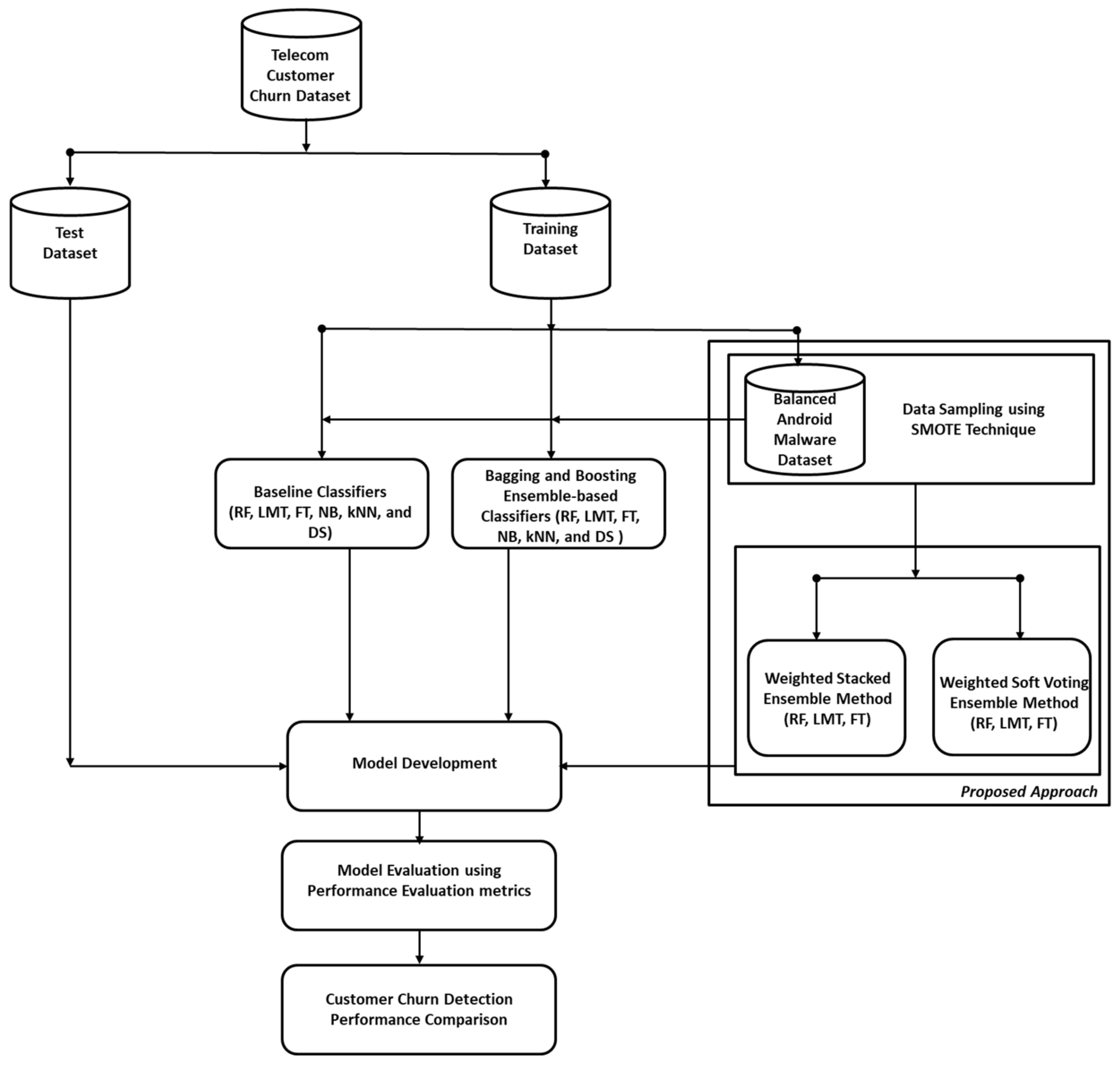
* The superior CCP performances are bold and type-faced, and the proposed DF models are designated by an asterisk.

present the comparison of CCP performances of DF models (LMT, FT, and RF) against ML classifiers (NB, kNN, and DS) on the original Datasets 1 and 2. The selected ML classifiers were chosen based on their prediction performances in ML tasks and distinct computational properties. In addition,

Table 5. The CCP performance of DF models and ML classifiers on Balanced (SMOTE) Dataset 1.

	Accuracy (%)	AUC	F-Measure	MCC
NB	78.33	0.866	0.883	0.567
kNN	88.27	0.881	0.883	0.767
DS	64.84	0.65	0.863	0.346
* LMT	93.60	0.971	0.966	0.872
* FT	94.83	0.975	0.968	0.897
* RF	92.14	0.943	0.945	0.843

* The superior CCP performances are bold and type-faced, and the proposed DF models are designated by an asterisk.

and

Table 6. The CCP performance of DF models and ML classifiers on Balanced (SMOTE) Dataset 2.

	Accuracy (%)	AUC	F-Measure	MCC
NB	77.21	0.825	0.772	0.545
kNN	83.91	0.839	0.839	0.678
DS	87.84	0.499	0.500	0.257
* LMT	91.59	0.896	0.876	0.752
* FT	94.26	0.973	0.942	0.883
* RF	90.32	0.880	0.503	0.806

* The superior CCP performances are bold and type-faced, and the proposed DF models are designated by an asterisk.

show the CCP performance of the DF models with the ML classifiers on SMOTE-balanced Dataset 1 and Dataset 2. The data sampling method (SMOTE) was deployed to address the inherent class imbalance problem in CCP datasets. In addition, the deployment of balanced datasets on the CCP models will indicate the impact of data sampling on CCP models. To develop effective CCP models, enhanced ensemble variants of the DT models (WSVEDFM and WSEDFM) were deployed on the original and balanced versions of Dataset 1 and Dataset 2. Specifically,

Table 7. The CCP performance of DF models and their Enhanced ensemble variants on original Dataset 1.

	Accuracy (%)	AUC	F-Measure	MCC
LMT	94.75	0.905	0.945	0.777
FP	94.42	0.905	0.942	0.763
RF	90.97	0.896	0.895	0.581
WSVEDFM	95.81	0.951	0.958	0.879
WSEDFM	95.53	0.948	0.955	0.865

,

Table 8. The CCP performance of DF models and their Enhanced ensemble variants on original Dataset 2.

	Accuracy (%)	AUC	F-Measure	MCC
LMT	89.86	0.5	?	?
FP	89.86	0.5	?	?
RF	89.49	0.508	0.850	0.003
WSVEDFM	89.86	0.555	0.855	0.030
WSEDFM	89.86	0.545	0.850	0.025

,

Table 9. The CCP performance of DF models and their Enhanced ensemble variants on balanced Dataset 1.

	Accuracy (%)	AUC	F-Measure	MCC
LMT	93.60	0.971	0.966	0.872
FP	94.83	0.975	0.968	0.897
RF	92.14	0.943	0.945	0.843
WSVEDFM	96.31	0.990	0.987	0.940
WSEDFM	96.31	0.989	0.983	0.946

and

Table 10. The CCP performance of DF models and their Enhanced ensemble variants on balanced Dataset 2.

	Accuracy (%)	AUC	F-Measure	MCC
LMT	91.59	0.896	0.876	0.752
FT	94.26	0.973	0.942	0.883
RF	90.32	0.880	0.503	0.806
WSVEDFM	96.57	0.988	0.965	0.981
WSEDFM	96.43	0.986	0.964	0.971

present the CCP performances of each of the DF models and their enhanced ensemble variants on the original and balanced studied customer churn datasets respectively. This analysis will show how the different DF models can work with imbalanced and balanced datasets. For a fair comparison, the CCP performances of DF models are further compared with renowned ensemble methods such as Bagging and Boosting. Finally, the CCP performances of the high-performing DF models are contrasted with current state-of-the-art CCP models. Consequently, the experimental results are aided by graphical representations to demonstrate the relevance of the observed experimental findings.

4.1. CCP Performance Comparison of the DF Models and ML Classifiers

In this section, the CCP performance of LMT, FT, and RF as DF models are compared with the ML classifiers on original and SMOTE-balanced Dataset 1 and Dataset 2 as outlined in Section 3.3 (Phase 1).

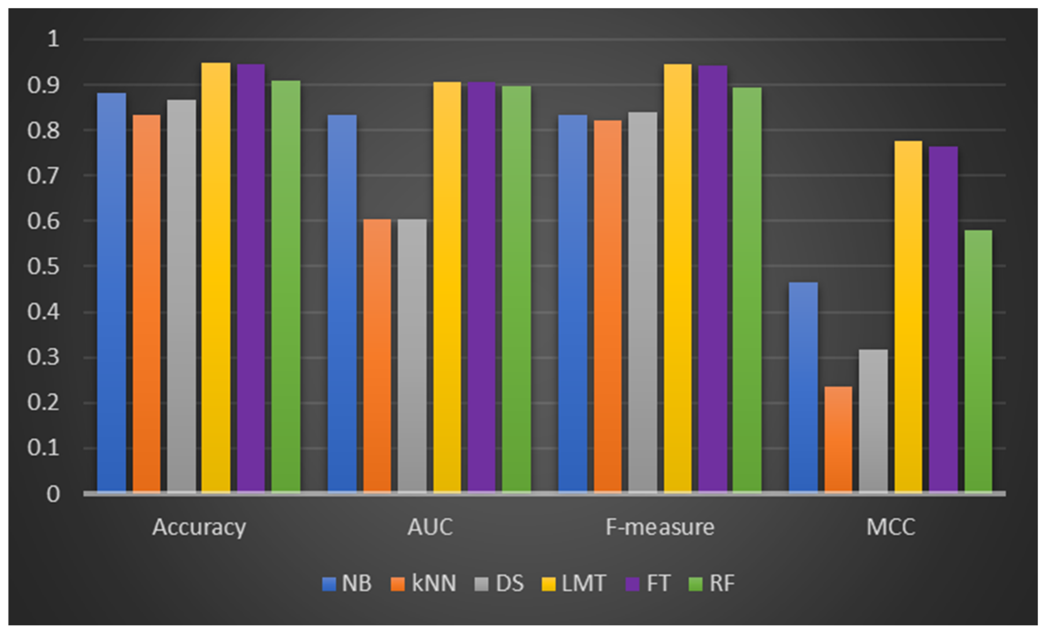
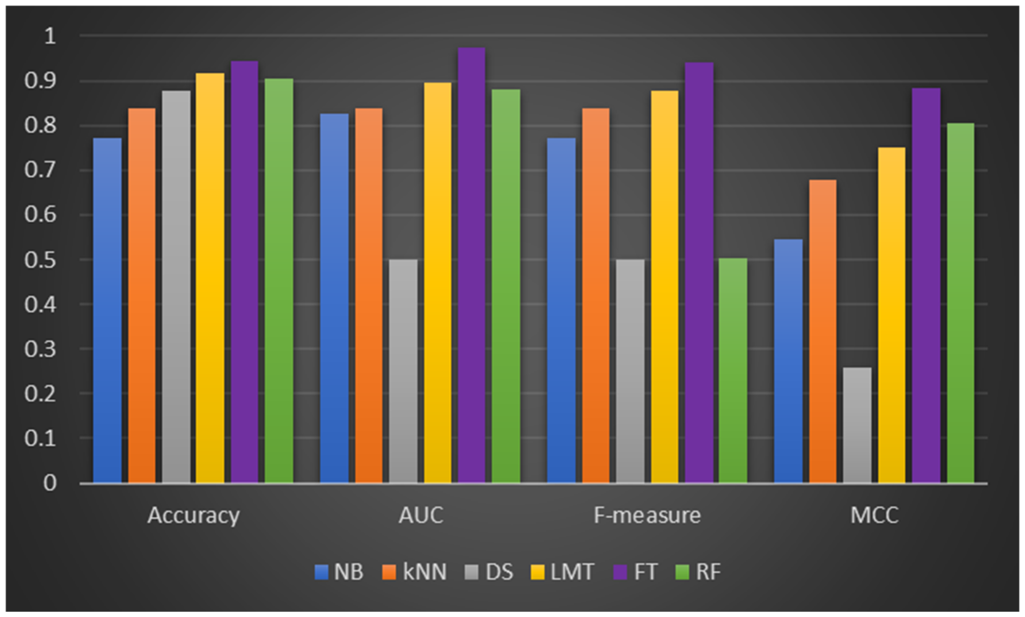
Table 3 illustrates the CCP performances of LMT, FT, and RF and the selected ML classifiers (NB, kNN, and DS) on Dataset 1 (Kaggle Dataset). It can be observed that the DF models were superior in prediction performances when compared to the experimented ML classifiers based on the studied performance metrics. Concerning accuracy values, LMT recorded the highest of 94.75% amongst the DF models, followed by FT and RF, respectively. As for the ML classifiers, NB performed best with 88.24% prediction accuracy. However, LMT, FT, and RF had +7.38, +7.0, and +3.09% accuracy increments compared to NB. The LMT, FT, and RF’s superior prediction accuracy values over NB, kNN, and DS, even on an imbalanced Dataset 1, highlights their resilience and usefulness for CCP. A similar occurrence can be observed regarding AUC values as the duo of LMT and FT both had the highest AUC values of 0.905 while RF had 0.896. The AUC values of these DF models were superior to that of NB (0.834), kNN (0.603), and DS (0.603). Also, the DF models obtained a strong ratio of sensitivity and recall, with LMT and FT having f-measure values of 0.945 and 00942, respectively. It is worth noting that the ML classifiers also had comparable f-measures, but they were still lower than those of the DF models. This observation confirms the performance stability of the DF models in CCP compared to experimented ML classifiers. In the case of the MCC values, the performances of the DF models are notably comparable, as LMT (0.777) was slightly better than FT (0.763). The other ML classifier had lower MCC values which indicate no conformity between the predicted and observed values. Figure 2 illustrates a graphical depiction of the CCP of the experimented models.

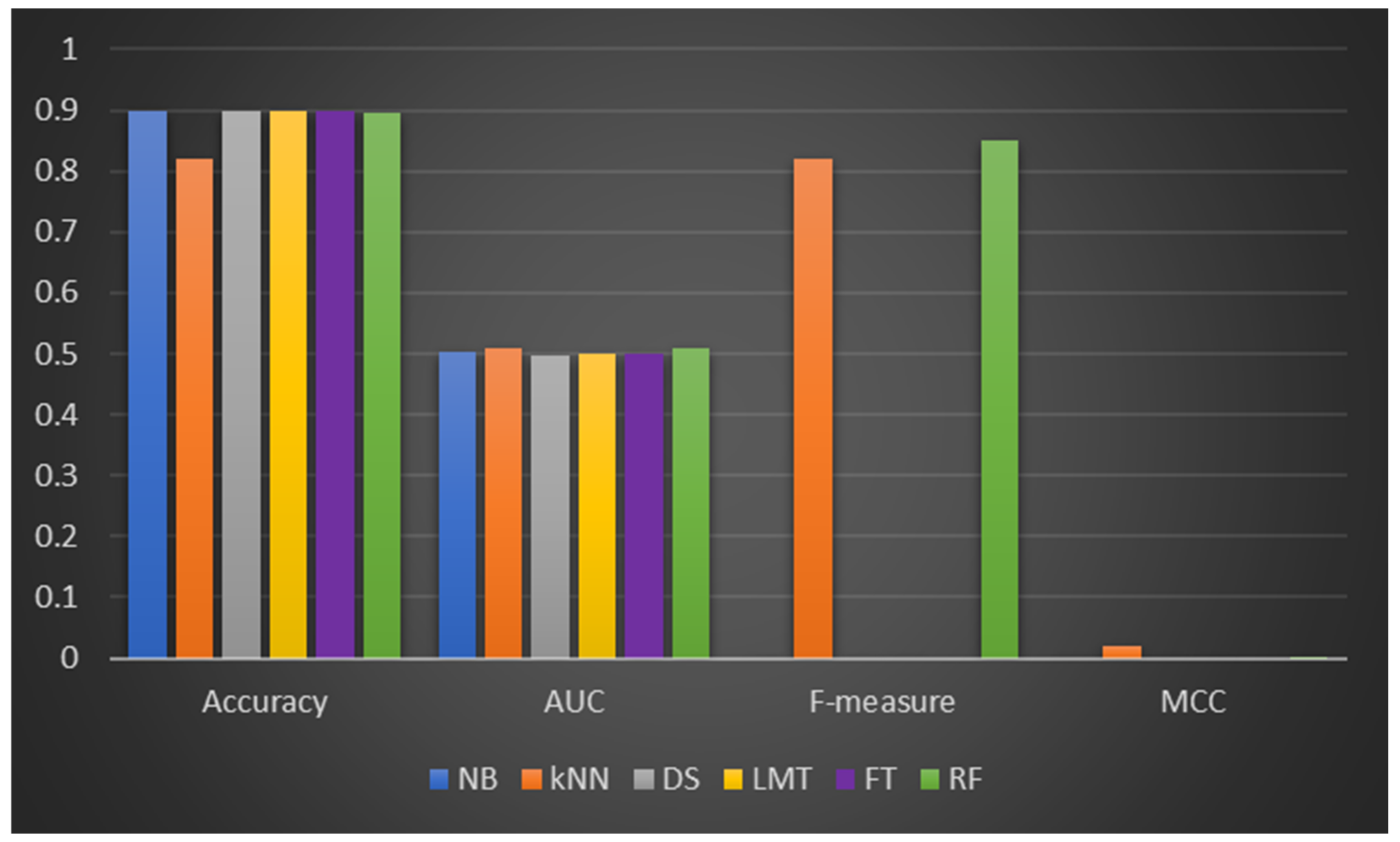
From Dataset 2 (presented in Table 4), the DF models had comparable performance to the ML classifiers in terms of accuracy, AUC, f-measure, and MCC values. It was also discovered that the DF model experimental results on Dataset 2 are somewhat lower than those of Dataset 1. LMT, FT, and NB had similar prediction accuracy values (89.86%), and their respective AUC values are average (LMT: 0.5, FT: 0.5, NB: 0.503). Also, it can be observed that the f-measure and MCC values of some of the implemented models (NB, DS, LMT, and FT) are missing, and some models recorded poor performance based on f-measure and MCC values. This observation can be attributed to the nature and data quality of Dataset 2. That is, the presence of class imbalance (as indicated in Table 2) (IR of 8.86) had a derogatory effect on the implemented DF and ML models. Figure 3 depicts DF’s and the ML classifiers’ CPP performances.

Based on the relative prediction performances of the DF models, which may have been affected by the latent class imbalance problem, the IR values for Dataset 1 and Dataset 2 are 5.9 and 8.86, respectively (See Table 2). Hence, this research work explored the prediction performances of the DF models and ML classifiers on balanced (SMOTE) CCP datasets. It is worth noting that the purpose of the SMOTE data sampling method is to eliminate the class imbalance issue as identified in Dataset 1 and Dataset 2 (See Table 2). Besides, the choice of SMOTE technique is due to its reported effectiveness and frequent deployment in current research. Specifically, Table 5 and Table 6 show the experimental results of DF models and ML classifiers on the balanced (SMOTE) Dataset 1 and Dataset 2, respectively.

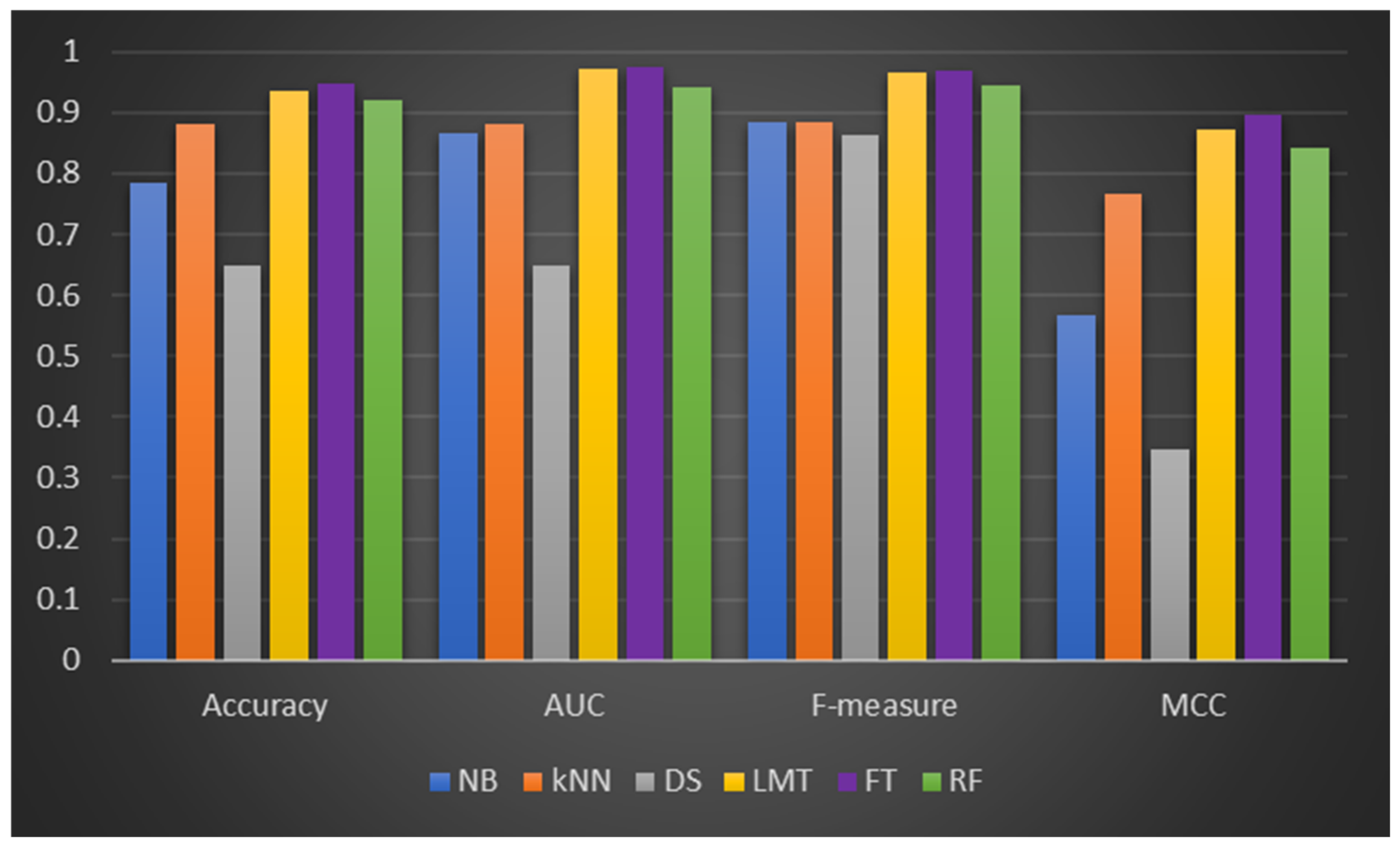
As seen in Table 5, the DF models (LMT, FT, and RF) are still superior to the ML classifiers (NB, kNN, and DS) on all performance parameters tested. FT and RF have a prediction accuracy of 94.83% and 92.14%, which are (+0.43%, +1.29%) better than FT and RF on original Dataset 1. Similar trends were observed in the performance of the DF models with AUC and MCC values. For instance, significant increments were observed in the AUC values of LMT (+7.3%), FT (+7.73%), and RF (+5.25%) on the balanced dataset compared with the original Dataset 1. Also, it was discovered that the ML classifiers had improved prediction performances based on AUC and MCC values. Specifically, the highest improvements in AUC values were attained by kNN (+46.1%) and DS (+7.79%). In addition, there was a notable increase in MCC value in NB (+21.9%), kNN (+223%), and DS (+9.15%). In terms of f-measure values, kNN (+7.55%) improved the most, followed by NB (+5.88%) and DS (+2.61%) in that order. However, in terms of the accuracy values, NB (−11.23%) and DS (−22.78%) had negative improvements, which may be due to the model overfitting observed in their respective CCP on the original dataset. This finding further affirms the importance of not using the accuracy value as the only performance metric since it does not represent the performance of an ML model adequately. On the SMOTE-balanced Dataset 1, the CCP performance of the DF models and the ML classifiers improved generally, but the DF models still achieved the highest overall performance. This finding could be related to deploying the data sampling (SMOTE) method to address the class imbalance issue in Dataset 1. Figure 4 depicts the performance of DF models and ML classifiers on CCP performance on the balanced Dataset 1.

Additionally, Table 6 displays the experimental results of the DF models and ML classifiers on balanced Dataset 2. The DF models still produced the best CCP performance based on all performance criteria analyzed. Balanced Dataset 1 showed a similar outcome to the experimental findings on balanced Dataset 2. That is, the DF models and the ML classifiers improved their CCP performance. As indicated in Table 6, FT (+4.89%), LMT (+1.63%), and RF (+0.93%) outperformed their respective CCP capabilities on the original Dataset 2. In terms of AUC values, the DF models (LMT (+79.2%), FT (+94.6%), and RF (+73.23%)) all showed significant improvement. The analysis based on the f-measure metric yielded similar results. Except for RF, the f-measure values of LMT, FT, and the ML classifiers improved. In terms of the MCC measure, the DF models showed significant incremental improvements in their respective MCC values, which showed a strong relationship between the observed and predicted outcome. Other ML classifiers (NB, kNN, and DS) also showed comparable MCC values. Figure 5 depicts the DF models and ML classifiers’ CCP performance on the balanced Dataset 2.

The following observations were noticed based on the preceding experimental results assessments on studied CCP datasets:

• The DF models (LMT, FT, and RF) outperformed the ML classifiers (NB, kNN, and DS) in CCP. It is worth noting that the experiment ML classifiers were chosen based on their use and performance in current CCP studies and ML tasks.
• The use of the SMOTE data sampling approach not only solved the class imbalance issue but also enhanced the CCP performances of the DF models and ML classifiers.
• The DF models can predict customer churn effectively with or without a data sampling strategy.

These experimental findings verify and substantiate using DF models (LMT, FT, and RF) for CCP. DF models enhanced ensemble variants (WSVEDFM and WSEDFM), on the other hand, were created to improve the DF models CCP performance. Section 4.2 presents and discusses the empirical assessment of experimental outcomes of WSVEDFM and WSEDFM methods.

4.2. CCP Performance Comparison of DF Models and Their Enhanced Ensemble Variants (WSVEDFM and WSEDFM)

This section compared the CCP performances of the DF models with their enhanced ensemble variants on the original and balanced CCP datasets. Specifically, Table 7 and Table 8 display the experimental results based on the original Dataset 1 and Dataset 2, while Table 9 and Table 10 show the results on balanced Dataset 1 and Dataset 2 as outlined in Section 3.3 (Phase 2).

Table 7 and Table 8 display the detection performances of LMT, FT, RF, WSVEDFM, and WSEDFM on original Dataset 1 and Dataset 2. On Dataset 1 (Table 7), both WSVEDFM and WSEDFM outperformed the DF models. WSVEDFM recorded a prediction accuracy value of 95.81%, an AUC value of 0.951, an f-measure value of 0.958, and an MCC value of 0.879. Likewise, WSEDFM showed a similar prediction accuracy value of 95.53%, an AUC value of 0.948, an f-measure value of 0.955, and an MCC value of 0.865. Significantly, the AUC value of 0.951 and 0.948 achieved by WSVEDFM and WSEDFM, respectively, demonstrate the efficacy of the two models (WSVEDFM and WSEDFM) in distinguishing churners from non-churners with a high degree of certainty. Similarly, relatively high MCC values achieved by WSVEDFM (0.879) and WSEDFM (0.865) indicate a positive correlation between the observed and the predicted CCP outcome. Also, from the experimental results on Dataset 2 (Table 8), WSVEDFM and WSEDFM were superior to the DF models on studied performance metrics. However, the performances of the models on Dataset 2 were not as effective as the performance on Dataset 1. This concern is due to the inherent data quality issues with Dataset 2. In addition, the CCP performance of LMT, FT, RF, WSVEDFM, and WSEDFM on balanced Dataset 1 and Dataset 2 were analyzed. This contraction is intended to determine the impact of deploying SMOTE data sampling method on the CCP performance of WSVEDFM and WSEDFM methods. That is, to investigate if the CCP performance of WSVEDFM and WSEDFM will be improved on balanced CCP datasets. Table 9 and Table 10 show the CCP performances of LMT, FT, RF, WSVEDFM, and WSEDFM on balanced Dataset 1 and Dataset 2.

On the balanced Dataset 1, WSVEDFM and WSEDFM outperformed LMT, FT, and RF, as shown in Table 9. For instance, WSVEDFM and WSEDFM demonstrated significant increment in prediction accuracy values above LMT (+2.89%), FT (+1.56%) and RF (+4.53%) respectively. Furthermore, WSVEDFM (0.990) and WSEDFM (0.989) demonstrated +1.54% and +1.44% increment in AUC values over FT (0.975) which had the best AUC values from the DF models respectively. Also, there is a significant difference in the MCC values of the WSVEDFM and WSEDFM over the individual DF models. WSVEDFM (0.981) and WSEDFM (0.971) showed +11.1% and +9.97% increment in MCC values over FT (0.883) which also happened to have the best MCCC values from the DF models. A similar trend was also detected in experimental results from the balanced Dataset 2. As shown in Table 10, WSVEDFM (96.57%) and WSEDFM (96.43%) recorded +2.45% and +2.30% increment in prediction accuracy values over FT (94.26%). Also, the AUC and MCC values of WSVEDFM (96.57%) and WSEDFM (96.43%) are superior to any DF models. Although amongst the DF models (LMT, FT, and RF), FT had the best CCP performance on both balanced Dataset 1 and Dataset 2; however, the DF models CCP performances are still outperformed by their enhanced ensemble variants (WSVEDFM and WSEDFM). Based on the results of the experimental tests reported here, it can be concluded that the upgraded variants (WSVEDFM and WSEDFM), particularly WSVEDFM, are more effective than any of the DF models (LMT, FT, and RF) in CCP tasks.

In addition, for more generalizable results and assessment, the CCP performances of WSVEDFM and WSEDFM methods are compared with prominent ensemble methods such as Bagging and Boosting. Bagging and Boosting ensemble methods have been reported to have a positive impact on its base model by amplifying prediction performance [65,66]. Section 4.3 presents a detailed analysis of the comparison of the proposed ensemble methods (WSVEDFM and WSEDFM) with Bagged and Boosted DF models on both original and balanced CCP datasets.

4.3. CCP Performance Comparison of Enhanced DFEnsemble Variants, Bagging and Boosting Ensemble Methods

In this section, further assessment and performance comparisons were conducted to validate the effectiveness of WSVEDFM and WSEDFM for CCP processes. Specifically, the proposed DF ensemble variants were compared with Bagged and Boosted DF models on both original and balanced (SMOTE) Dataset 1 and Dataset 2.

Table 11. The CCP performance comparison of WSVEDFM and WSEDFM with Bagged and Boosted DF models on Dataset 1.

	Accuracy (%)	AUC	F-Measure	MCC
BaggedLMT	95.21	0.914	0.951	0.801
BaggedFT	95.44	0.918	0.953	0.807
BaggedRF	90.16	0.898	0.881	0.533
BoostedLMT	94.18	0.911	0.932	0.756
BoostedFT	93.49	0.903	0.940	0.721
BoostedRF	91.36	0.899	0.900	0.602
* WSVEDFM	95.81	0.951	0.958	0.879
* WSEDFM	95.53	0.948	0.955	0.865

* The superior CCP performances are bold and type-faced, and the proposed DF models are designated by an asterisk.

,

Table 12. The CCP performance comparison of WSVEDFM and WSEDFM with Bagged and Boosted DF models on Dataset 2.

	Accuracy (%)	AUC	F-Measure	MCC
BaggedLMT	87.20	0.515	0.843	0.012
BaggedFT	89.86	0.497	?	?
BaggedRF	89.72	0.521	0.850	0.001
BoostedLMT	85.14	0.523	0.834	0.007
BoostedFT	85.44	0.534	0.836	0.016
BoostedRF	88.72	0.516	0.849	0.016
* WSVEDFM	89.86	0.555	0.855	0.030
* WSEDFM	89.86	0.545	0.850	0.025

* The superior CCP performances are bold and type-faced, and the proposed DF models are designated by an asterisk.

,

Table 13. The CCP performance of DF models and their Enhanced ensemble variants on balanced Dataset 1.

	Accuracy (%)	AUC	F-Measure	MCC
BaggedLMT	95.50	0.986	0.955	0.910
BaggedFT	95.96	0.985	0.960	0.919
BaggedRF	92.30	0.971	0.923	0.846
BoostedLMT	95.43	0.984	0.954	0.909
BoostedFT	95.36	0.984	0.954	0.907
BoostedRF	92.30	0.973	0.923	0.847
* WSVEDFM	96.31	0.990	0.987	0.940
* WSEDFM	96.31	0.989	0.983	0.946

* The superior CCP performances are bold and type-faced, and the proposed DF models are designated by an asterisk.

and

Table 14. The CCP performance of DF models and their Enhanced ensemble variants on balanced Dataset 2.

	Accuracy (%)	AUC	F-Measure	MCC
BaggedLMT	88.56	0.934	0.886	0.771
BaggedFT	88.56	0.928	0.886	0.771
BaggedRF	90.06	0.945	0.901	0.801
BoostedLMT	87.99	0.932	0.880	0.760
BoostedFT	88.26	0.934	0.883	0.766
BoostedRF	89.97	0.930	0.900	0.799
* WSVEDFM	96.57	0.988	0.965	0.981
* WSEDFM	96.43	0.986	0.964	0.971

* The superior CCP performances are bold and type-faced, and the proposed DF models are designated by an asterisk.

outline the CCP performance and comparison of WSVEDFM and WSEDFM with the Bagged DF and Boosted DF models on original and balanced CCP datasets.

As shown in Table 10 and Table 11, the Bagged and Boosted DF models had comparable performances as the WSVEDFM and WSEDFM on Dataset 1 and Dataset 2, respectively. In some cases, the differences in the prediction accuracy and f-measure values of the proposed DF ensemble variants and the Bagged and Boosted DF modes are insignificant. However, the WSVEDFM and WSEDFM are still superior in performance. For instance, WSVEDFM (0.951) and WSEDFM (0.948) had a +3.59% and +3.27% increment in AUC values over Bagged FT (0.918), which had the highest AUC value amongst the Bagged and Boosted DF models. A similar trend was observed with the MCC values with WSVEDFM (0.879) and WSEDFM (0.865), recording a +9.74% and +7.99% over Bagged FT (0.801). Contrary to the findings from Table 11, the CCP performance of the studied models on Dataset 2, as shown in Table 12, is relatively good. This could be related to the observed data quality problem (high IR) in Dataset 2. However, on a general note, the WSVEDFM and WSEDFM outperformed the Bagged and Boosted DF models, although the CCP performances of the Bagged DF models are better than the Boosted DF models. This finding can be due to the independent and parallel mode of model development in the Bagging method, which reduces variances amongst its base models and avoids model overfitting. In addition, the CCP performances of WSVEDFM and WSEDFM with Bagged and Boosted DF models on balanced Dataset 1 and Dataset 2 were compared. Table 13 and Table 14 display the CCP performances of WSVEDFM, WSEDFM, Bagged DF models, and Boosted DF models on balanced Dataset 1 and Dataset 2, respectively.

As shown in Table 13 and Table 14, it can be observed that there are significant improvements in the performances of the WSVEDFM and WSEDFM over the Bagged and Boosted DF models on the balanced Dataset 1 and Dataset 2. Specifically, from Table 13, WSVEDFM and WSEDFM had a +0.36% increment in prediction accuracy values more than the best performer (Bagged FT) in this case. Also, a +2.29% and +2.94% increment in MCC values of WSVEDFM and WSEDFM over Bagged FT was observed. In the balanced Dataset 2 (See Table 14), WSVEDFM and WSEDFM had a +7.23% and +7.07% increase in prediction accuracy value over BaggedRF. Based on MCC values, WSVEDFM and WSEDFM achieved +22.47% and +21.22% increment over Bagged RF. From the Bagged and Boosted DF models, BaggedRF had the best performance on balanced Dataset 2.

In summary, based on the observed experimental findings on the analyses of the experimental results of the WSVEDFM, WSEDFM, Bagged DF models, and Boosted DF models on the balanced Dataset 1 and Dataset 2, it is fair to assert that the enhanced DF ensemble variants are more suitable for CCP than the prominent Bagged and Boosted DF models. Nonetheless, the CCP performances of the DF models and their enhanced ensemble variants are compared with existing CCP models in Section 4.4.

4.4. CCP Performance Comparison of DF Models and Their Enhanced Ensemble Variants with Existing CCP Methods

For comprehensiveness, the CCP performances of the LMT, FT, RF, WSVEDFM, and WSEDFM are compared to those of current CCP solutions.

Table 15. The CCP performance of proposed DF methods and existing models on Dataset 1.

	Accuracy (%)	AUC	F-Measure	MCC
* LMT	93.60	0.971	0.966	0.872
* FT	94.83	0.975	0.968	0.897
* RF	92.14	0.943	0.945	0.843
* WSVEDFM	96.31	0.990	0.987	0.940
* WSEDFM	96.31	0.989	0.983	0.946
Tavassoli and Koosha [59] (BNNGA)	86.81	-	0.688	-
Ahmad, Jafar and Aljoumaa [60] (SNA + XGBOOST)	-	0.933	-	-
Jain, et al. [67] (CNN+VAE)	90.00	-	0.930	-
Saghir, Bibi, Bashir and Khan [36] (BaggedMLP)	94.15	-	0.874	-
Jain, et al. [68] (LogitBoost)	85.24	0.717	0.810	0.160
Jeyakarthic and Venkatesh [69] (P-AGBPNN)	91.71	-	0.951
Praseeda and Shivakumar [70] (PFLICM)	95.41	-	-	-
Dalli [71] (Hyper-Parameterized DL with RMSProp)	86.50	-	-	-

* The superior CCP performances are bold and type-faced, and the proposed DF models are designated by an asterisk.

and

Table 16. The CCP performance of proposed DF methods and existing models on Dataset 2.

	Accuracy (%)	AUC	F-Measure	MCC
* LMT	91.59	0.896	0.876	0.752
* FT	94.26	0.973	0.942	0.883
* RF	90.32	0.880	0.503	0.806
* WSVEDFM	96.57	0.988	0.965	0.981
* WSEDFM	96.43	0.986	0.964	0.971
Tavassoli and Koosha [59](BBNGA)	77.50	-	0.773	-
Saghir, Bibi, Bashir and Khan [36] (Bagging)	80.80	-	0.784	-
Shaaban, Helmy, Khedr and Nasr [62] (SVM)	83.70	-	-	-
Bilal, Almazroi, Bashir, Khan and Almazroi [37] (KMed+GBT+DL+DL+Voting)	94.06	-	0.745	-
Bilal, Almazroi, Bashir, Khan and Almazroi [37] (KMed+GBT+DL+DL+Stacking)	94.65	-	0.796	-
Bilal, Almazroi, Bashir, Khan and Almazroi [37] (KMed+GBT+DL+DL+Adaboost)	94.70	-	0.806	-
Bilal, Almazroi, Bashir, Khan and Almazroi [37] (KMed+GBT+DL+DL+Bagging)	94.12	-	0.746	-

* The superior CCP performances are bold and type-faced, and the proposed DF models are designated by an asterisk.

show the CCP performance of proposed DF models and current CCP solutions on Dataset 1 and Dataset 2, respectively.

As presented in Table 15, the CCP performance of the DF models and its enhanced ensemble variants are compared with that of Tavassoli and Koosha [59], Ahmad, Jafar and Aljoumaa [60], Jain, Khunteta and Shrivastav [67], Saghir, Bibi, Bashir and Khan [36], Jain, Khunteta and Srivastava [68], Jeyakarthic and Venkatesh [69], Praseeda and Shivakumar [70], and Dalli [71] on Dataset 1. These existing CCP models range from ensemble methods to sophisticated DL methods. For instance, Tavassoli and Koosha [59] developed a hybrid ensemble (BNNGA) method for CCP, which had a prediction accuracy value of 86.81% and an f-measure value of 0.688. Similarly, Saghir, Bibi, Bashir and Khan [36] deployed a Bagged MLP, while Jain, Khunteta and Srivastava [68] used a LogitBoost approach for CCP. However, the CCP performances of the DF models and their enhanced ensemble variants are superior to these ensemble-based CCP models in most cases. Using another approach, Ahmad, Jafar and Aljoumaa [60] combined Social Network Analysis (SNA) and XGBoost for CCP. The SNA was deployed to generate new features for the CCP. Also, Jain, Khunteta and Shrivastav [67] enhanced CNN with a Variable Auto-Encoder (VAE). Although their AUC value of SNA+XGBoost is quite significant and the prediction accuracy and f-measure of CNN+VAE is above 90%, there CCP performance are still less than that of the proposed methods. Praseeda and Shivakumar [70] used a probabilistic-based fuzzy local information c-means (PFLICM) for CCP. PFLICM is a clustering based approach and it had a prediction accuracy value of 95.41%. In addition, Dalli [71] hyper-parameterized DL+RMSProp and Jeyakarthic and Venkatesh [69] designed an adaptive Gain with Back Propagation Neural Networks (P-AGBPNN) for CCP process. These methods are based on enhanced DL techniques with comparable CCP performance. In summary, the proposed DF models and its enhanced ensemble variants are superior to examined existing CCP models with different computational processes on Dataset 1.

Furthermore, Table 16 presents the CCP performance comparison of the DF models and their enhanced ensemble variants with CCP solutions of Tavassoli and Koosha [59], Saghir, Bibi, Bashir and Khan [36], Shaaban, Helmy, Khedr and Nasr [62], and Bilal, Almazroi, Bashir, Khan and Almazroi [37]. These existing CCP solutions were developed with Dataset 2 as utilized in this study. Specifically, Saghir, Bibi, Bashir and Khan [36] deployed a Bagging ensemble approach for CCP with a prediction accuracy value of 80.80% and an f-measure value of 0.784. Also, Shaaban, Helmy, Khedr and Nasr [62] used a parameterized SVM for CCP. The relatively low CCP performances of these methods, when compared with the proposed DF methods, could result from the failure to address the class imbalance problem in their respective studies. In addition, Bilal, Almazroi, Bashir, Khan and Almazroi [37] combined clustering and classification methods for CCP. Specifically, Kmediod was combined with a gradient boosting technique (GBT), and the resulting model is evaluated using diverse ensemble techniques such as Bagging, Stacking, Voting, and Adaboost. While the CCP performance of their method was comparable to the proposed DF models, the high computational complexity of their methods is a concern. Regardless, the DF models and their enhanced ensemble variants are superior to the existing CCP models evaluated on Dataset 2.

4.5. Answers to Research Questions

Based on the investigations, the following findings were obtained to answer the RQs posed in the introduction section.

RQ1:

How efficient are the investigated DF models (LMT, FT, and RF) in CCP as compared with prominent ML classifiers

The experimental findings showed that the investigated DF models (LMT, FT, and RF) outperformed the prominent ML classifiers in terms of CCP performance. This higher CCP performance was demonstrated on both Dataset 1 and Dataset 2.

RQ2:

How efficient are the DF models’ enhanced ensemble variations in CCP?

The WSVEDFM and WSEDFM outperformed the individual DF models and the Bagged and Boosted individual DF models on both the original and balanced (SMOTE) CCP datasets. Furthermore, the SMOTE methodology we used addressed the intrinsic class imbalance issue seen in the CCP datasets and improved the CCP performances of the suggested DF models, notably the WSVEDFM and WSEDFM techniques.

RQ3:

How do the suggested DF models and their ensemble variations compare to existing state-of-the-art CCP solutions?

Furthermore, observable findings indicated that the suggested DF models (LMT, FT, and RF) and enhanced ensemble variants (WSVEDFM and WSEDFM) outperformed current CCP solutions on the studied CCP datasets in most cases.

5. Threats to Validity

This section describes the validity threats faced during the experiment. According to Zhang, Moro and Ramos [11], CCP is becoming increasingly relevant, and evaluating and limiting threats to the validity of experimental results is an important component of any empirical study.

External validity: The potential to generalize the experimental research is important to its validity. The kind and number of datasets utilized in the experimental phase may affect the generalizability of research findings in several ways. As a result, two major and frequently used CCP datasets with a diverse set of features (Kaggle (20) and UCI (18)) have been identified. These datasets are freely accessible to the public and are widely used for training and evaluating CCP methods. Furthermore, this study provided a complete analysis of the experimentation method, which might assist in the reproducibility and validity of its methodological approaches to diverse CCP datasets.

Internal validity: This concept highlights the significance and regularity of datasets, ML techniques, and empirical analysis. As such, notable ML approaches developed and used in previous research are used in this study. The ML techniques were selected for their merit (effectiveness) and diversity. In addition, to prevent unexpected errors in empirical findings, the investigated CCP models were systematically implemented (trained) on the chosen CCP datasets using the CV approach, and each experiment was repeated 10 times for thoroughness. However, future studies may examine other model assessment methodologies and tactics.

Construct validity: This issue is related to the choice of evaluation criteria used to evaluate the efficiency of CCP models that have been investigated. Accuracy, AUC, f-measure, and MCC were all used in this research work. These metrics offered a detailed and complete empirical analysis of the CCP models used in the experiment. Furthermore, the DF models we used for CCP were developed specifically to determine the churning process and status.

6. Conclusions and Future Works

In this research work, DF models and their enhanced ensemble variants were developed for customer churn prediction. Specifically, LMT, FT, RF, Weighted Soft Voting Ensemble Decision Forest Method (WSVEDFM), and Weighted Stacking Ensemble Decision Forest Method (WSEDFM) were developed and tested on original (imbalanced) and balanced (SMOTE) telecommunication customer churn datasets. Experiments were conducted to examine the efficacy and applicability of the suggested DF models. Empirical results showed that the DF models outperformed base-line ML classifiers such as NB, kNN, and DS on the imbalanced and balanced Kaggle and UCI telecommunication customer churn datasets. This discovery validates the applicability of DF models for CCP. Furthermore, the enhanced ensemble versions of the DF models (WSEDFM and WSVEDFM) beat Bagged and Boosted models on imbalanced and balanced datasets, indicating their usefulness in CCP. Furthermore, the suggested DF models (LMT, FT, RF, WSVEDFM, and WSEDFM) outperformed the best models in the literature on Kaggle and UCI telecommunication customer churn datasets. As a result, this research recommends deploying suggested DF models for CCP.

As a continuation of this research work, we intend to investigate the spotting and removal of outliers and extreme values, which could contribute to improved outcomes (CCP models). Also, the characteristics of projected customer churns were not explored in this research work, though they may be relevant to corporations deciding whether to retain certain churn customers. As a result, good churn clients may have a higher lifetime value. Nonetheless, we hope to address these critical concerns in future research work.

References

1. Lalwani, P.; Mishra, M.K.; Chadha, J.S.; Sethi, P. Customer churn prediction system: A machine learning approach. Computing 2022, 104, 271–294. [Google Scholar] [CrossRef]
2. Arowolo, M.O.; Abdulsalam, S.O.; Saheed, Y.K.; Afolayan, J.O. Customer Churn Prediction in Telecommunication Industry Using Decision Tree and Artificial Neural Network Algorithms. Indones. J. Electr. Eng. Inform. 2022, 10, 431–440. [Google Scholar]
3. Park, S.-H.; Kim, M.-Y.; Kim, Y.-J.; Park, Y.-H. A Deep Learning Approach to Analyze Airline Customer Propensities: The Case of South Korea. Appl. Sci. 2022, 12, 1916. [Google Scholar] [CrossRef]
4. Arifin, A.S. Telecommunication service subscriber churn likelihood prediction analysis using diverse machine learning model. In Proceedings of the 2020 3rd International Conference on Mechanical, Electronics, Computer, and Industrial Technology (MECnIT), Medan, Indonesia, 25–27 June 2020; pp. 24–29. [Google Scholar]
5. Domingos, E.; Ojeme, B.; Daramola, O. Experimental analysis of hyperparameters for deep learning-based churn prediction in the banking sector. Computation 2021, 9, 34. [Google Scholar] [CrossRef]
6. Xiong, Y.; Tao, J.; Zhao, S.; Wu, R.; Shen, X.; Lyu, T.; Fan, C.; Hu, Z.; Zhao, S.; Pan, G. Explainable AI for Cheating Detection and Churn Prediction in Online Games. IEEE Trans. Games 2022. [Google Scholar] [CrossRef]
7. Sabourin, V.; Jabo, J.T. IoT Benefits and Growth Opportunities for the Telecom Industry: Key Technology Drivers for Companies; CRC Press: Boca Raton, FL, USA, 2022. [Google Scholar]
8. Brânduşoiu, I.; Toderean, G.; Beleiu, H. Methods for churn prediction in the pre-paid mobile telecommunications industry. In Proceedings of the 2016 International conference on communications (COMM), Bucharest, Romania, 9–10 June 2016; pp. 97–100. [Google Scholar]
9. Cao, S.; Liu, W.; Chen, Y.; Zhu, X. Deep learning based customer churn analysis. In Proceedings of the 2019 11th International Conference on Wireless Communications and Signal Processing (WCSP), Xi’an, China, 23–25 October 2019; pp. 1–6. [Google Scholar]
10. Mishra, A.; Reddy, U.S. A comparative study of customer churn prediction in telecom industry using ensemble based classifiers. In Proceedings of the 2017 International Conference on Inventive Computing and Informatics (ICICI), Coimbatore, India, 23–24 November 2017; pp. 721–725. [Google Scholar]
11. Zhang, T.; Moro, S.; Ramos, R.F. A Data-Driven Approach to Improve Customer Churn Prediction Based on Telecom Customer Segmentation. Future Internet 2022, 14, 94. [Google Scholar] [CrossRef]
12. Jain, H.; Khunteta, A.; Srivastava, S. Telecom churn prediction and used techniques, datasets and performance measures: A review. Telecommun. Syst. 2021, 76, 613–630. [Google Scholar] [CrossRef]
13. Amin, A.; Anwar, S.; Adnan, A.; Nawaz, M.; Alawfi, K.; Hussain, A.; Huang, K. Customer churn prediction in the telecommunication sector using a rough set approach. Neurocomputing 2017, 237, 242–254. [Google Scholar] [CrossRef]
14. Amin, A.; Al-Obeidat, F.; Shah, B.; Adnan, A.; Loo, J.; Anwar, S. Customer churn prediction in telecommunication industry using data certainty. J. Bus. Res. 2019, 94, 290–301. [Google Scholar] [CrossRef]
15. Wael Fujo, S.; Subramanian, S.; Ahmad Khder, M. Customer Churn Prediction in Telecommunication Industry Using Deep Learning. Inf. Sci. Lett. 2022, 11, 24. [Google Scholar]
16. Beeharry, Y.; Tsokizep Fokone, R. Hybrid approach using machine learning algorithms for customers’ churn prediction in the telecommunications industry. Concurr. Comput. Pract. Exp. 2022, 34, e6627. [Google Scholar] [CrossRef]
17. AlShourbaji, I.; Helian, N.; Sun, Y.; Alhameed, M. Anovel HEOMGA Approach for Class Imbalance Problem in the Application of Customer Churn Prediction. SN Comput. Sci. 2021, 2, 464. [Google Scholar] [CrossRef]
18. Leevy, J.L.; Khoshgoftaar, T.M.; Bauder, R.A.; Seliya, N. A survey on addressing high-class imbalance in big data. J. Big Data 2018, 5, 42. [Google Scholar] [CrossRef]
19. Wang, L.; Xu, S.; Wang, X.; Zhu, Q. Addressing class imbalance in federated learning. In Proceedings of the AAAI Conference on Artificial Intelligence, Palo Alto, CA, USA, 2–9 February 2021; pp. 10165–10173. [Google Scholar]
20. Balogun, A.; Basri, S.; Abdulkadir, S.; Adeyemo, V.; Imam, A.; Bajeh, A. Software defect prediction: Analysis of class imbalance and performance stability. J. Eng. Sci. Technol. 2019, 14, 3294–3308. [Google Scholar]
21. Balogun, A.O.; Lafenwa-Balogun, F.B.; Mojeed, H.A.; Adeyemo, V.E.; Akande, O.N.; Akintola, A.G.; Bajeh, A.O.; Usman-Hamza, F.E. SMOTE-based homogeneous ensemble methods for software defect prediction. In Proceedings of the International Conference on Computational Science and its Applications, Cagliari, Italy, 1–4 July 2020; pp. 615–631. [Google Scholar]
22. Sagi, O.; Rokach, L. Explainable decision forest: Transforming a decision forest into an interpretable tree. Inf. Fusion 2020, 61, 124–138. [Google Scholar] [CrossRef]
23. Brandusoiu, I.; Toderean, G. Churn prediction in the telecommunications sector using support vector machines. Margin 2013, 1, x1. [Google Scholar] [CrossRef]
24. Hossain, M.M.; Miah, M.S. Evaluation of different SVM kernels for predicting customer churn. In Proceedings of the 2015 18th International Conference on Computer and Information Technology (ICCIT), Dhaka, Bangladesh, 21–23 December 2015; pp. 1–4. [Google Scholar]
25. Mohammad, N.I.; Ismail, S.A.; Kama, M.N.; Yusop, O.M.; Azmi, A. Customer churn prediction in telecommunication industry using machine learning classifiers. In Proceedings of the 3rd International Conference on Vision, Image and Signal Processing, Vancouver, BC, Canada, 26–28 August 2019; pp. 1–7. [Google Scholar]
26. Kirui, C.; Hong, L.; Cheruiyot, W.; Kirui, H. Predicting customer churn in mobile telephony industry using probabilistic classifiers in data mining. Int. J. Comput. Sci. Issues 2013, 10, 165. [Google Scholar]
27. Abbasimehr, H.; Setak, M.; Tarokh, M. A neuro-fuzzy classifier for customer churn prediction. Int. J. Comput. Appl. 2011, 19, 35–41. [Google Scholar]
28. Zhang, C.; Li, H.; Xu, G.; Zhu, X. Customer churn model based on complementarity measure and random forest. In Proceedings of the 2021 International Conference on Computer, Blockchain and Financial Development (CBFD), Nanjing, China, 23–25 April 2021; pp. 95–99. [Google Scholar]
29. Karanovic, M.; Popovac, M.; Sladojevic, S.; Arsenovic, M.; Stefanovic, D. Telecommunication services churn prediction-deep learning approach. In Proceedings of the 2018 26th Telecommunications Forum (TELFOR), Belgrade, Serbia, 20–21 November 2018; pp. 420–425. [Google Scholar]
30. Spanoudes, P.; Nguyen, T. Deep learning in customer churn prediction: Unsupervised feature learning on abstract company independent feature vectors. arXiv 2017, arXiv:1703.03869. [Google Scholar]
31. Cenggoro, T.W.; Wirastari, R.A.; Rudianto, E.; Mohadi, M.I.; Ratj, D.; Pardamean, B. Deep learning as a vector embedding model for customer churn. Procedia Comput. Sci. 2021, 179, 624–631. [Google Scholar] [CrossRef]
32. Prashanth, R.; Deepak, K.; Meher, A.K. High accuracy predictive modelling for customer churn prediction in telecom industry. In Proceedings of the International Conference on Machine Learning and Data Mining in Pattern Recognition, New York, NY, USA, 15–20 July 2017; pp. 391–402. [Google Scholar]
33. Agrawal, S.; Das, A.; Gaikwad, A.; Dhage, S. Customer churn prediction modelling based on behavioural patterns analysis using deep learning. In Proceedings of the 2018 International Conference on Smart Computing and Electronic Enterprise (ICSCEE), Selangor, Malaysia, 11–12 July 2018; pp. 1–6. [Google Scholar]
34. Shabankareh, M.J.; Shabankareh, M.A.; Nazarian, A.; Ranjbaran, A.; Seyyedamiri, N. A Stacking-Based Data Mining Solution to Customer Churn Prediction. J. Relatsh. Mark. 2022, 21, 124–147. [Google Scholar] [CrossRef]
35. Xu, T.; Ma, Y.; Kim, K. Telecom churn prediction system based on ensemble learning using feature grouping. Appl. Sci. 2021, 11, 4742. [Google Scholar] [CrossRef]
36. Saghir, M.; Bibi, Z.; Bashir, S.; Khan, F.H. Churn prediction using neural network based individual and ensemble models. In Proceedings of the 2019 16th International Bhurban Conference on Applied Sciences and Technology (IBCAST), Islamabad, Pakistan, 8–12 January 2019; pp. 634–639. [Google Scholar]
37. Bilal, S.F.; Almazroi, A.A.; Bashir, S.; Khan, F.H.; Almazroi, A.A. An ensemble based approach using a combination of clustering and classification algorithms to enhance customer churn prediction in telecom industry. PeerJ Comput. Sci. 2022, 8, e854. [Google Scholar] [CrossRef]
38. Landwehr, N.; Hall, M.; Frank, E. Logistic model trees. Mach. Learn. 2005, 59, 161–205. [Google Scholar] [CrossRef]
39. Adeyemo, V.E.; Balogun, A.O.; Mojeed, H.A.; Akande, N.O.; Adewole, K.S. Ensemble-based logistic model trees for website phishing detection. In Proceedings of the International Conference on Advances in Cyber Security, Penang, Malaysia, 8–9 December 2020; pp. 627–641. [Google Scholar]
40. Balogun, A.O.; Adewole, K.S.; Raheem, M.O.; Akande, O.N.; Usman-Hamza, F.E.; Mabayoje, M.A.; Akintola, A.G.; Asaju-Gbolagade, A.W.; Jimoh, M.K.; Jimoh, R.G. Improving the phishing website detection using empirical analysis of Function Tree and its variants. Heliyon 2021, 7, e07437. [Google Scholar] [CrossRef]
41. Gama, J. Functional trees. Mach. Learn. 2004, 55, 219–250. [Google Scholar] [CrossRef]
42. Balogun, A.O.; Adewole, K.S.; Bajeh, A.O.; Jimoh, R.G. Cascade generalization based functional tree for website phishing detection. In Proceedings of the International Conference on Advances in Cyber Security, Penang, Malaysia, 24–25 August 2021; pp. 288–306. [Google Scholar]
43. Cutler, A.; Cutler, D.R.; Stevens, J.R. Random forests. In Ensemble Machine Learning; Springer: Berlin/Heidelberg, Germany, 2012; pp. 157–175. [Google Scholar]
44. Antoniadis, A.; Lambert-Lacroix, S.; Poggi, J.-M. Random forests for global sensitivity analysis: A selective review. Reliab. Eng. Syst. Saf. 2021, 206, 107312. [Google Scholar] [CrossRef]
45. Balogun, A.O.; Mojeed, H.A.; Adewole, K.S.; Akintola, A.G.; Salihu, S.A.; Bajeh, A.O.; Jimoh, R.G. Optimized decision forest for website phishing detection. In Proceedings of the Computational Methods in Systems and Software, Online, 1 October 2021; pp. 568–582. [Google Scholar]
46. Rokach, L. Decision forest: Twenty years of research. Inf. Fusion 2016, 27, 111–125. [Google Scholar] [CrossRef]
47. Akintola, A.G.; Balogun, A.O.; Capretz, L.F.; Mojeed, H.A.; Basri, S.; Salihu, S.A.; Usman-Hamza, F.E.; Sadiku, P.O.; Balogun, G.B.; Alanamu, Z.O. Empirical Analysis of Forest Penalizing Attribute and Its Enhanced Variations for Android Malware Detection. Appl. Sci. 2022, 12, 4664. [Google Scholar] [CrossRef]
48. Alsariera, Y.A.; Elijah, A.V.; Balogun, A.O. Phishing website detection: Forest by penalizing attributes algorithm and its enhanced variations. Arab. J. Sci. Eng. 2020, 45, 10459–10470. [Google Scholar] [CrossRef]
49. Balogun, A.O.; Odejide, B.J.; Bajeh, A.O.; Alanamu, Z.O.; Usman-Hamza, F.E.; Adeleke, H.O.; Mabayoje, M.A.; Yusuff, S.R. Empirical Analysis of Data Sampling-Based Ensemble Methods in Software Defect Prediction. In Proceedings of the 22nd International Conference on Computational Science and Its Applications (ICCSA), Malaga, Spain, 4–7 July 2022; pp. 363–379. [Google Scholar]
50. Balogun, A.O.; Bajeh, A.O.; Orie, V.A.; Yusuf-Asaju, W.A. Software Defect Prediction Using Ensemble Learning: An ANP Based Evaluation Method. FUOYE J. Eng. Technol. 2018, 3, 50–55. [Google Scholar] [CrossRef]
51. Jimoh, R.; Balogun, A.; Bajeh, A.; Ajayi, S. A PROMETHEE based evaluation of software defect predictors. J. Comput. Sci. Its Appl. 2018, 25, 106–119. [Google Scholar]
52. Xu, Z.; Liu, J.; Yang, Z.; An, G.; Jia, X. The impact of feature selection on defect prediction performance: An empirical comparison. In Proceedings of the 2016 IEEE 27th International Symposium on Software Reliability Engineering (ISSRE), Ottawa, ON, Canada, 23–27 October 2016; pp. 309–320. [Google Scholar]
53. Yu, Q.; Jiang, S.; Zhang, Y. The performance stability of defect prediction models with class imbalance: An empirical study. IEICE Trans. Inf. Syst. 2017, 100, 265–272. [Google Scholar] [CrossRef]
54. Yadav, S.; Shukla, S. Analysis of k-fold cross-validation over hold-out validation on colossal datasets for quality classification. In Proceedings of the 2016 IEEE 6th International Conference on Advanced Computing (IACC), Bhimavaram, India, 27–28 February 2016; pp. 78–83. [Google Scholar]
55. Arlot, S.; Lerasle, M. Choice of V for V-fold cross-validation in least-squares density estimation. J. Mach. Learn. Res. 2016, 17, 7256–7305. [Google Scholar]
56. Balogun, A.O.; Basri, S.; Jadid, S.A.; Mahamad, S.; Al-momani, M.A.; Bajeh, A.O.; Alazzawi, A.K. Search-Based Wrapper Feature Selection Methods in Software Defect Prediction: An Empirical Analysis. In Proceedings of the Computer Science Online Conference, Zlin, Czech Republic, 15 July 2020; pp. 492–503. [Google Scholar]
57. Hall, M.; Frank, E.; Holmes, G.; Pfahringer, B.; Reutemann, P.; Witten, I.H. The WEKA data mining software: An update. ACM SIGKDD Explor. Newsl. 2009, 11, 10–18. [Google Scholar] [CrossRef]
58. Crawley, M.J. The R Book; John Wiley & Sons: Hoboken, NJ, USA, 2012. [Google Scholar]
59. Tavassoli, S.; Koosha, H. Hybrid ensemble learning approaches to customer churn prediction. Kybernetes 2021, 51, 1062–1088. [Google Scholar] [CrossRef]
60. Ahmad, A.K.; Jafar, A.; Aljoumaa, K. Customer churn prediction in telecom using machine learning in big data platform. J. Big Data 2019, 6, 28. [Google Scholar] [CrossRef]
61. Faris, H. A hybrid swarm intelligent neural network model for customer churn prediction and identifying the influencing factors. Information 2018, 9, 288. [Google Scholar] [CrossRef]
62. Shaaban, E.; Helmy, Y.; Khedr, A.; Nasr, M. A proposed churn prediction model. Int. J. Eng. Res. Appl. 2012, 2, 693–697. [Google Scholar]
63. Jain, H.; Khunteta, A.; Srivastava, S. Churn prediction in telecommunication using logistic regression and logit boost. Procedia Comput. Sci. 2020, 167, 101–112. [Google Scholar] [CrossRef]
64. Chicco, D.; Jurman, G. The advantages of the Matthews correlation coefficient (MCC) over F1 score and accuracy in binary classification evaluation. BMC Genom. 2020, 21, 6. [Google Scholar] [CrossRef] [PubMed]
65. Zhu, Q. On the performance of Matthews correlation coefficient (MCC) for imbalanced dataset. Pattern Recognit. Lett. 2020, 136, 71–80. [Google Scholar] [CrossRef]
66. Alsariera, Y.A.; Balogun, A.O.; Adeyemo, V.E.; Tarawneh, O.H.; Mojeed, H.A. Intelligent tree-based ensemble approaches for phishing website detection. J. Eng. Sci. Technol. 2022, 17, 563–582. [Google Scholar]
67. Odejide, B.J.; Bajeh, A.O.; Balogun, A.O.; Alanamu, Z.O.; Adewole, K.S.; Akintola, A.G.; Salihu, S.A.; Usman-Hamza, F.E.; Mojeed, H.A. An Empirical Study on Data Sampling Methods in Addressing Class Imbalance Problem in Software Defect Prediction. In Proceedings of the Computer Science Online Conference, Online, 26–30 April 2022; pp. 594–610. [Google Scholar]
68. Jain, H.; Khunteta, A.; Shrivastav, S.P. Telecom Churn Prediction Using Seven Machine Learning Experiments integrating Features engineering and Normalization. Res. Sq. 2021, preprint. [Google Scholar]
69. Jeyakarthic, M.; Venkatesh, S. An effective customer churn prediction model using adaptive gain with back propagation neural network in cloud computing environment. J. Res. Lepid. 2020, 51, 386–399. [Google Scholar]
70. Praseeda, C.; Shivakumar, B. Fuzzy particle swarm optimization (FPSO) based feature selection and hybrid kernel distance based possibilistic fuzzy local information C-means (HKD-PFLICM) clustering for churn prediction in telecom industry. SN Appl. Sci. 2021, 3, 613. [Google Scholar] [CrossRef]
71. Dalli, A. Impact of Hyperparameters on Deep Learning Model for Customer Churn Prediction in Telecommunication Sector. Math. Probl. Eng. 2022, 2022, 4720539. [Google Scholar] [CrossRef]
Figure 1. Experimental Framework.
Applsci 12 08270 g001
Figure 2. CCP Performance of DF models and ML Classifiers on Dataset 1.
Applsci 12 08270 g002
Figure 3. CCP Performance of DF models and ML Classifiers on Dataset 2.
Applsci 12 08270 g003
Figure 4. CCP Performance of DF models and ML Classifiers on balanced (SMOTE) Dataset 1.
Applsci 12 08270 g004
Figure 5. CCP Performance of DF models and ML Classifiers on balanced (SMOTE) Dataset 2.
Applsci 12 08270 g005