
Serial Decoders-Based Auto-Encoders for Image Reconstruction


Abstract
:Featured Application
Abstract
1. Introduction
2. Related Research
3. Theory
3.1. Notations and Abbreviations
3.2. Recall of Classical Auto-Encoders
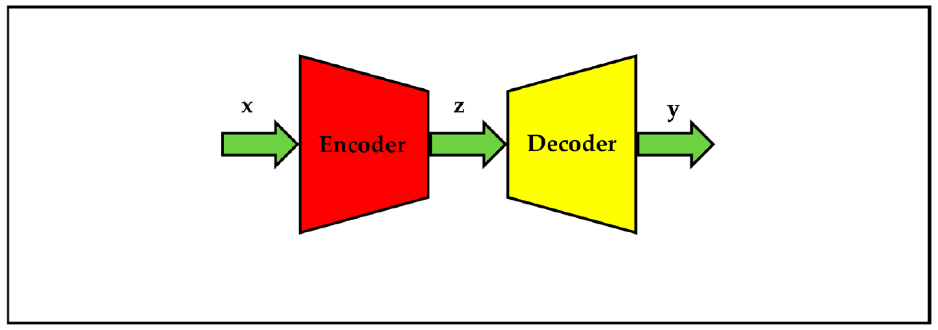
- x is the high-dimensional input data. Taking image data as an example, x is the normalized version of original image for the convenience of numerical computation; each element of the original image is an integer in the range [0, 255]; each element of x is a real number in the range [0, 1] or [−1, +1]; x with elements in the range [0, 1] can be understood as probability variables; x can also be regarded as a vector which is a reshaping version of an image matrix.
- z is the low-dimensional representation in a latent space.
- y is the high-dimensional data, such as a reconstruction image.
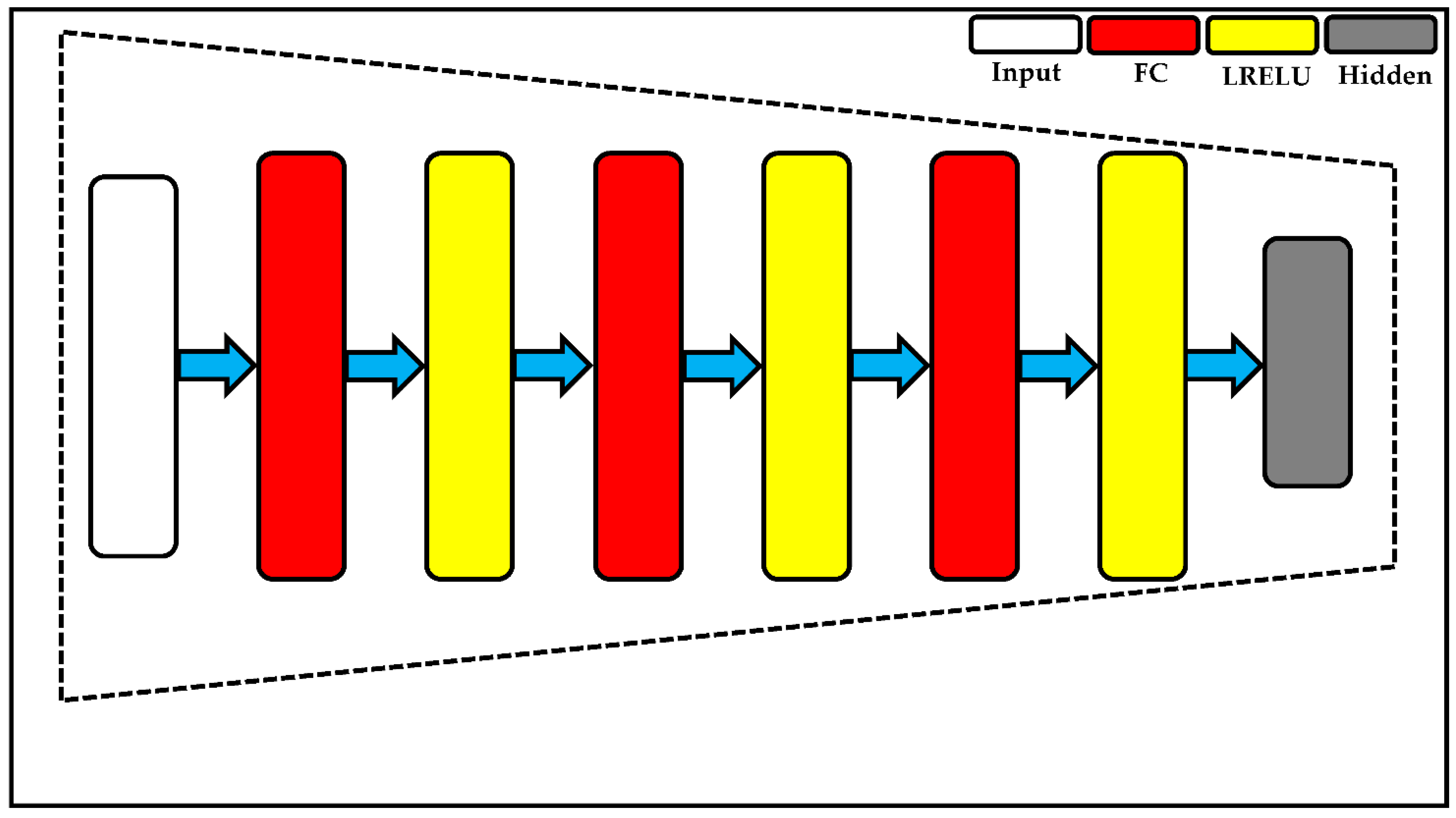
- E is the encoder.
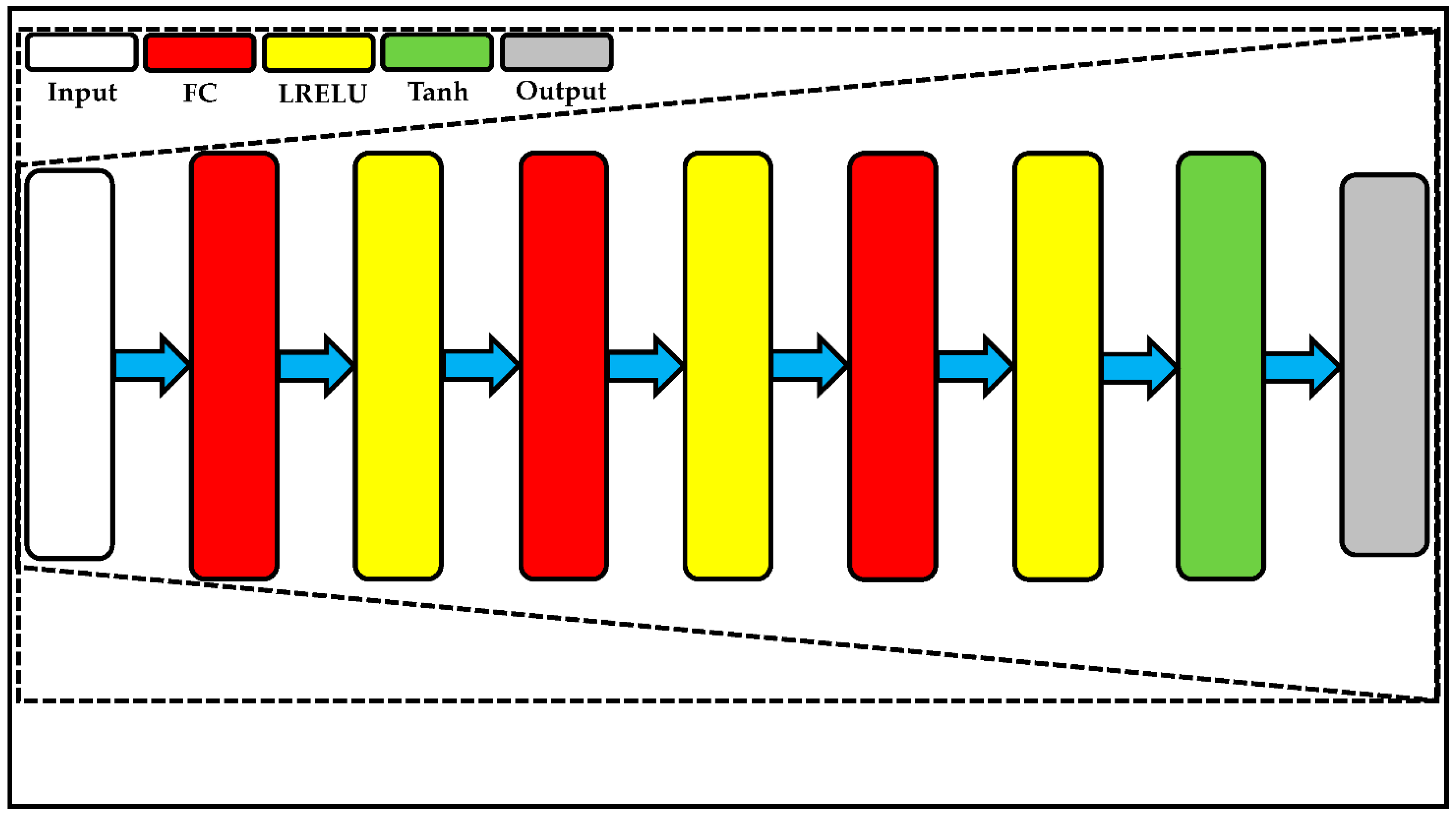
- D is the decoder.
- H is the dimension of x or y; for image data, H is equal to the product of image width and height.
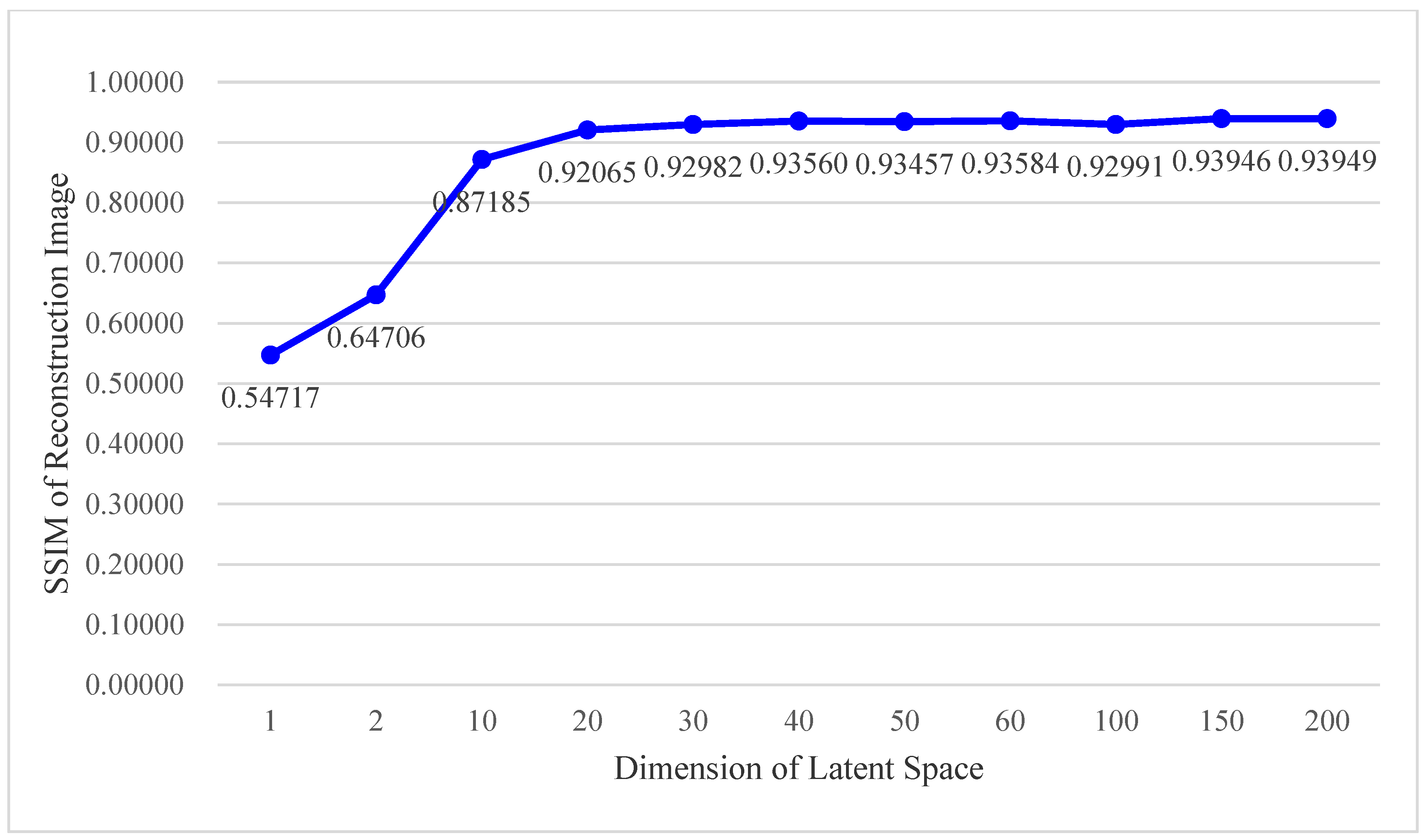
- L is the dimension of z and L is far less than H.
- θ are the parameters of auto-encoders, including the parameters of the encoder and decoder.
- Cz is the constraint on low-dimensional representation z; for example, z satisfies a given probability distribution; it has been considered to match a known distribution by classical adversarial auto-encoders, variational auto-encoders, and Wasserstein auto-encoders.
- zg is a related variable which meets a given distribution.
- δz is a small constant.
- Cy is the constraint on high-dimensional reconstruction data y; for instance, y meets a prior of local smoothness or non-local similarity. Auto-encoders require y to reconstruct x based on the prior to a great extent; other constraints, such as sparsity and low-rank properties of high-dimensional reconstruction data can also be utilized; hereby, sparse prior is taken as an example.
- Dy is a matrix of sparse dictionary.
- sy is a vector of sparse coefficients.
- λy is a small constant.
- δy is a small constant.
3.3. Proposed Cascade of Decoders-Based Auto-Encoders
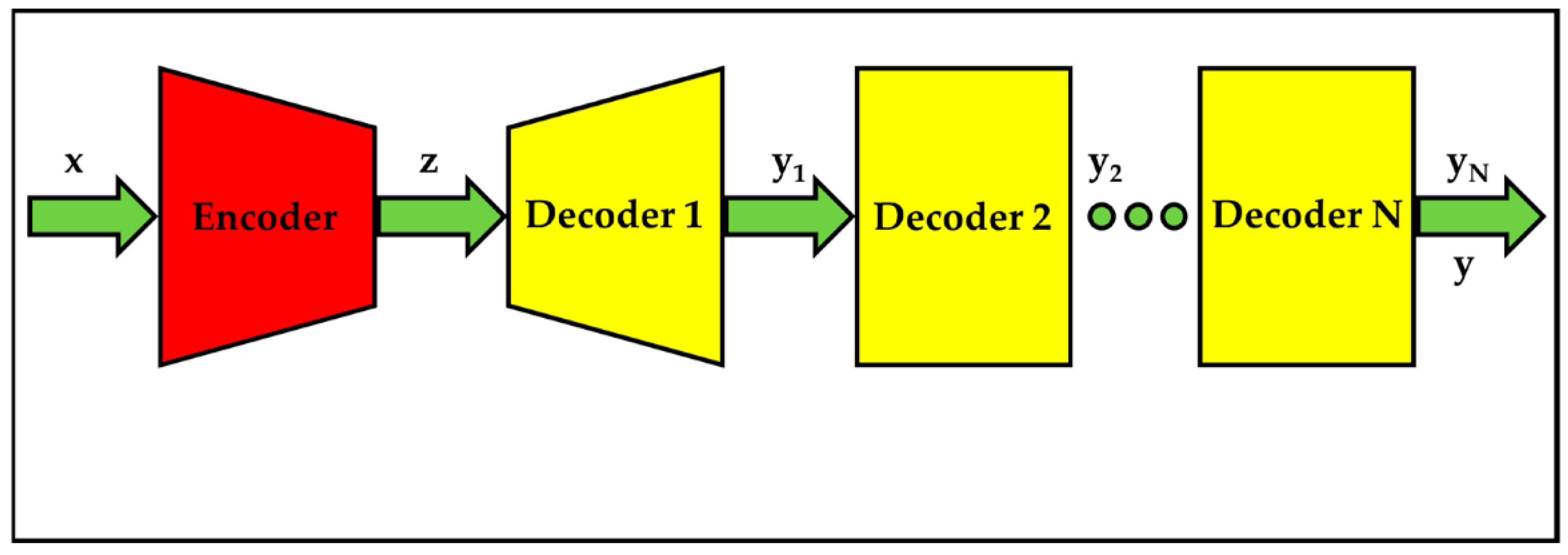
- Dn is the nth decoder;
- yn is the reconstruction data of Dn.
- θ are the parameters of cascade decoders-based auto-encoders;
- Cyn is the constraint on yn.
- θ1 are the parameters of encoder and decoder 1;
- θ2, …, and θN are the parameters of decoder 2 to N.
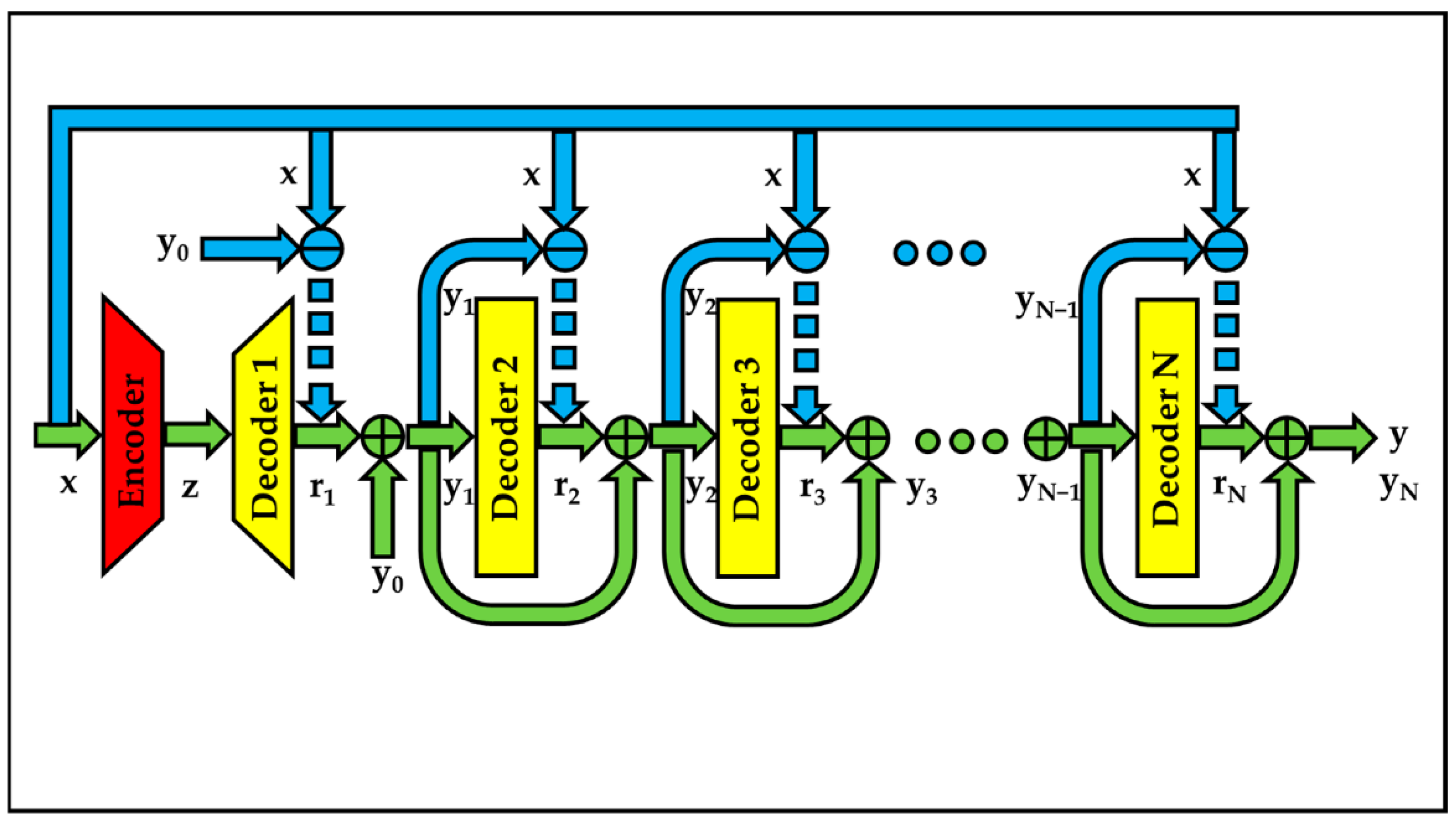
3.3.1. Residual Cascade Decoders-Based Auto-Encoders
- rn is the residual sample between x and yn;
- y0 is the zero sample;
- y is the final reconstruction sample.
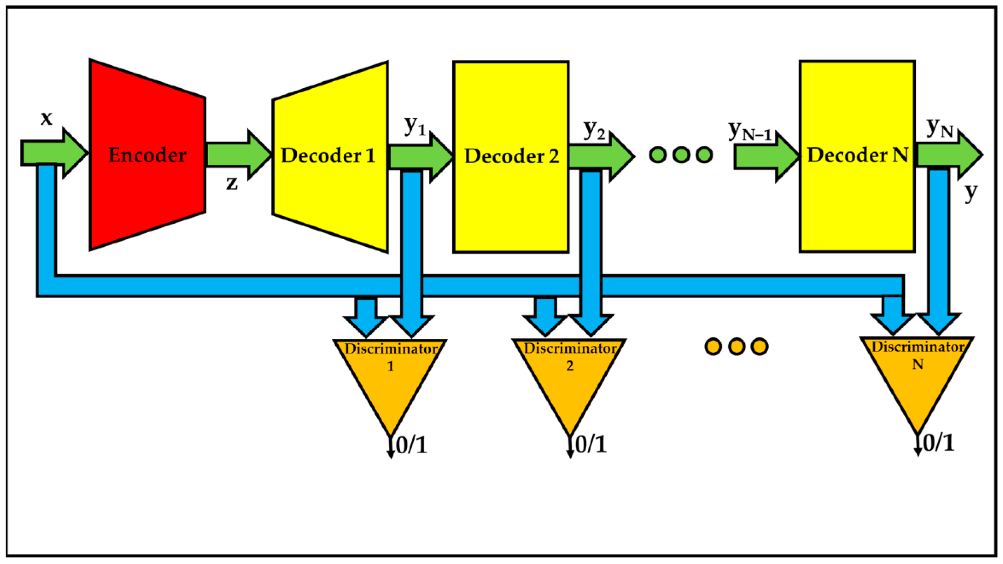
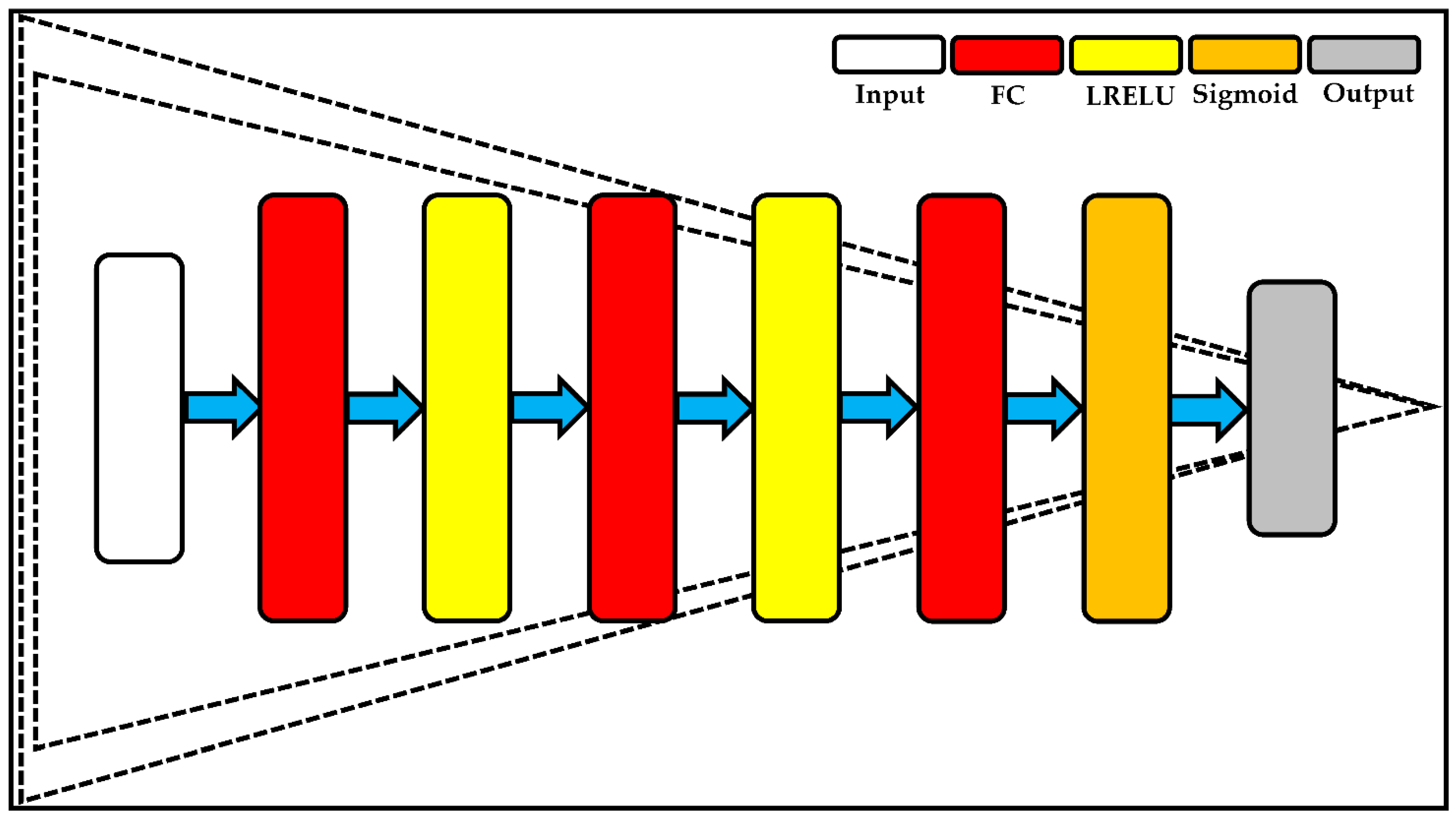
3.3.2. Adversarial Cascade Decoders-Based Auto-Encoders
- DCn is the nth discriminator;
- αn is a constant;
- βn is a constant;
- ε is a small positive constant;
- M is the mean operator.
3.3.3. Residual-Adversarial Cascade Decoders-Based Auto-Encoders
3.4. Adversarial Auto-Encoders
3.4.1. Reminiscence of Classical Adversarial Auto-Encoders
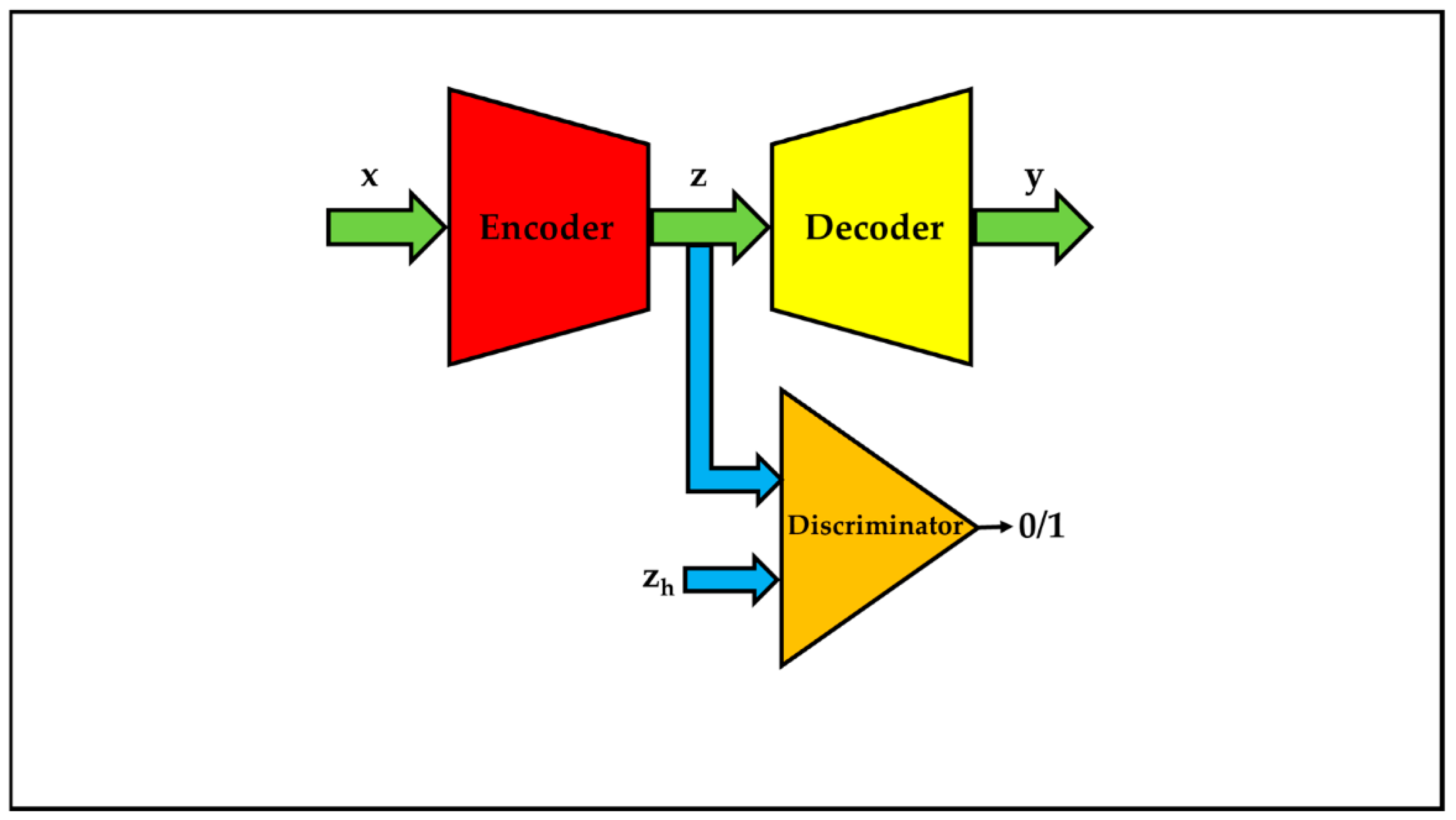
- zh is the variable related to z which satisfies a given distribution;
- DC is the discriminator.
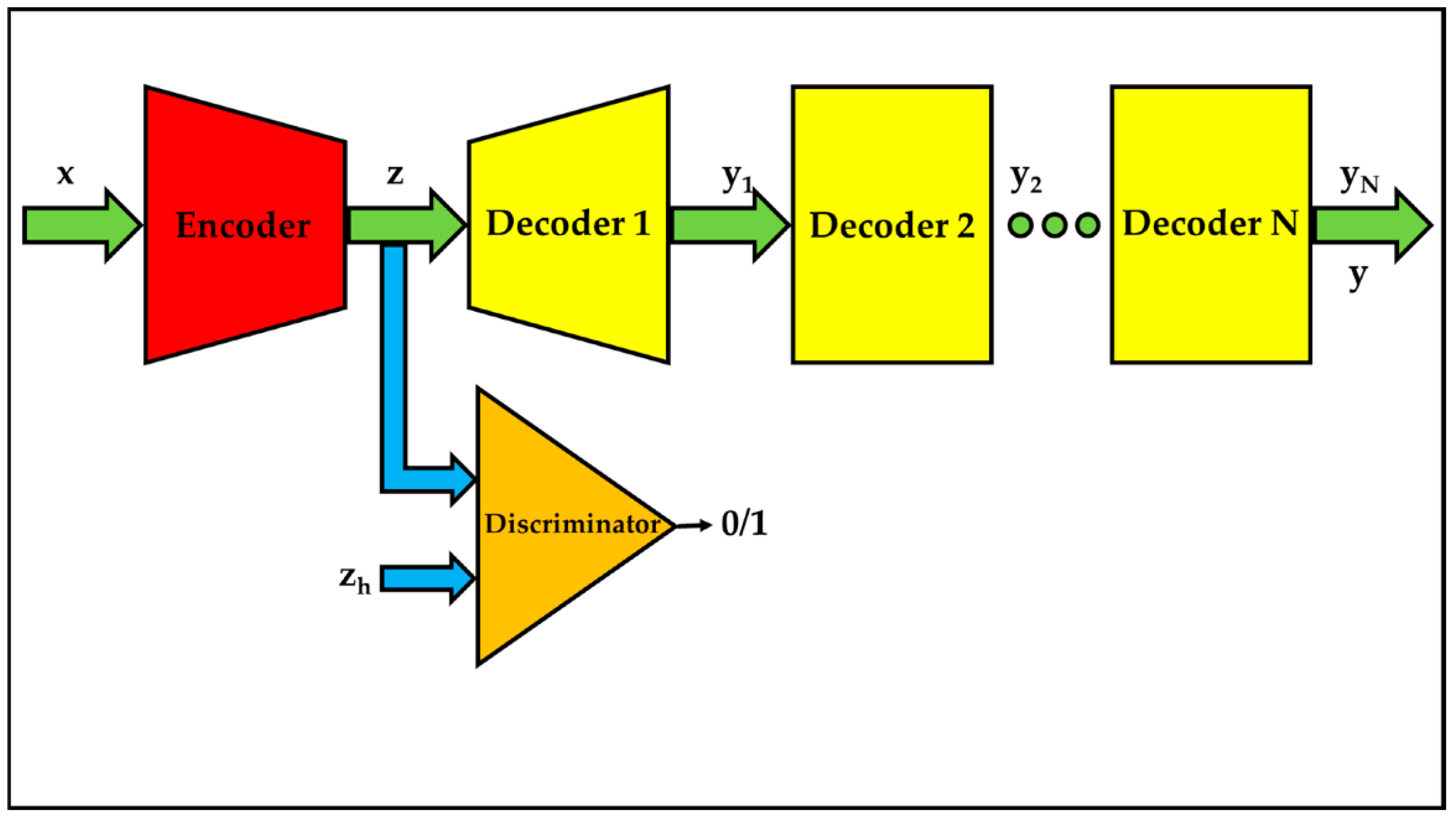
3.4.2. Proposed Cascade Decoders-Based Adversarial Auto-Encoders
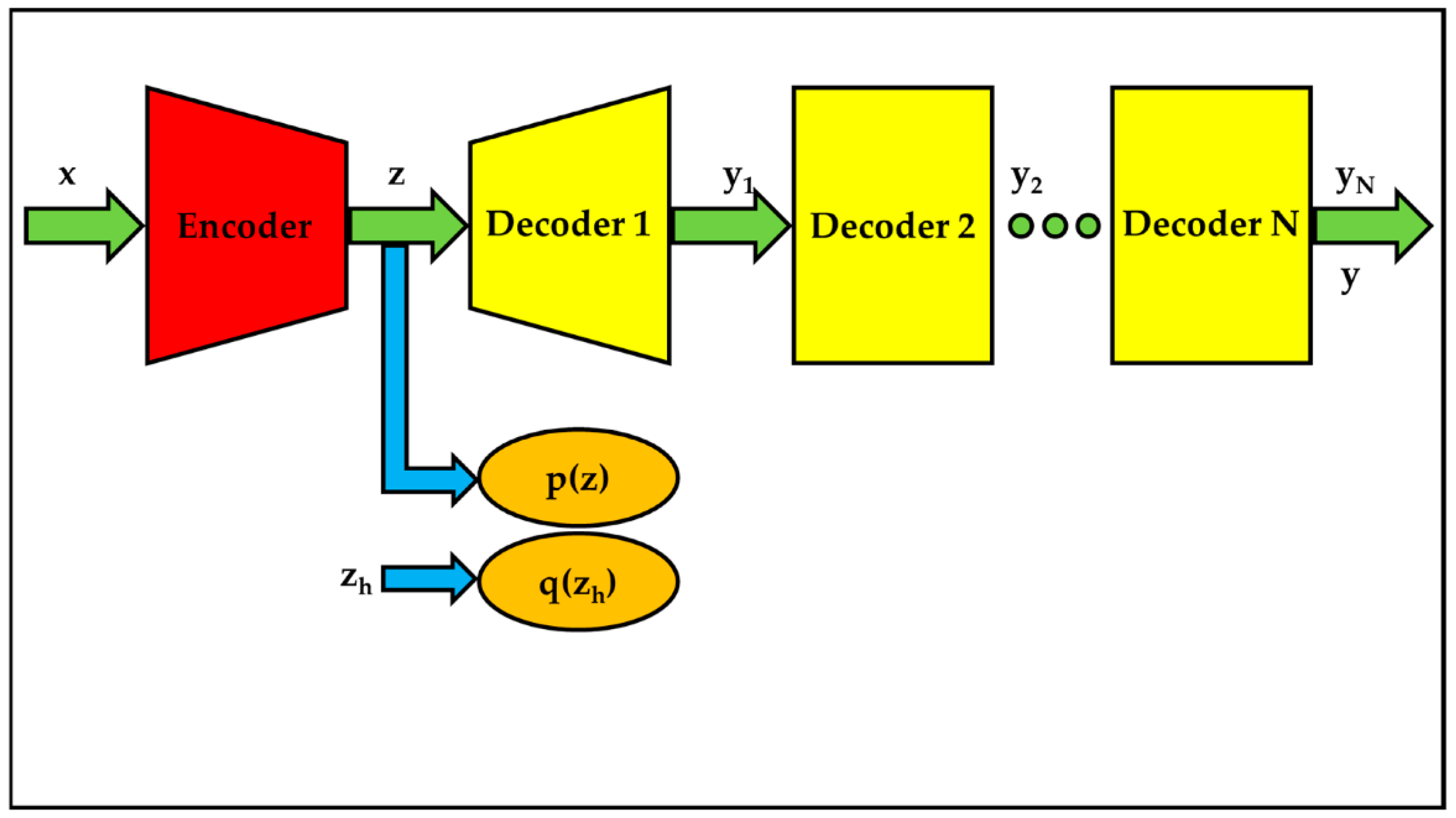
3.5. Variational Auto-Encoders
3.5.1. Remembrance of Classical Variational Auto-Encoders

- KL(·) is the Kullback–Leibler divergence;
- q(zh) is the given distribution of zh;
- p(z) is the distribution of z.
3.5.2. Proposed Cascade Decoders-Based Variational Auto-Encoders
3.6. Wasserstein Auto-Encoders
3.6.1. Recollection of Classical Wasserstein Auto-Encoders
- Wz is the regularizer between distribution p(z) and q(zh);
- Wy is the reconstruction cost.
3.6.2. Proposed Cascade Decoders-Based Wasserstein Auto-Encoders
3.7. Pseudocodes of Cascade Decoders-Based Auto-Encoders
| Algorithm 1: The pseudo codes of cascade decoders-based auto-encoders. |
| Input: x: the training data |
| I: the total number of iteration |
| N: the total number of sub minimization problem |
| Initialization: i =1 |
| Training: |
| While i <= I |
| i++ |
| n = 1 |
| While n <= N |
| n++ |
| resolve the nth sub problem in Equations (5), (7), (10), (12), (17), (20) or (23) |
| Output: |
| θ: the parameters of deep neural networks |
| z: the representations of hidden space |
| y1, …, yN: the output of cascade decoders |
| y: the output of the last decoder |
4. Experiments
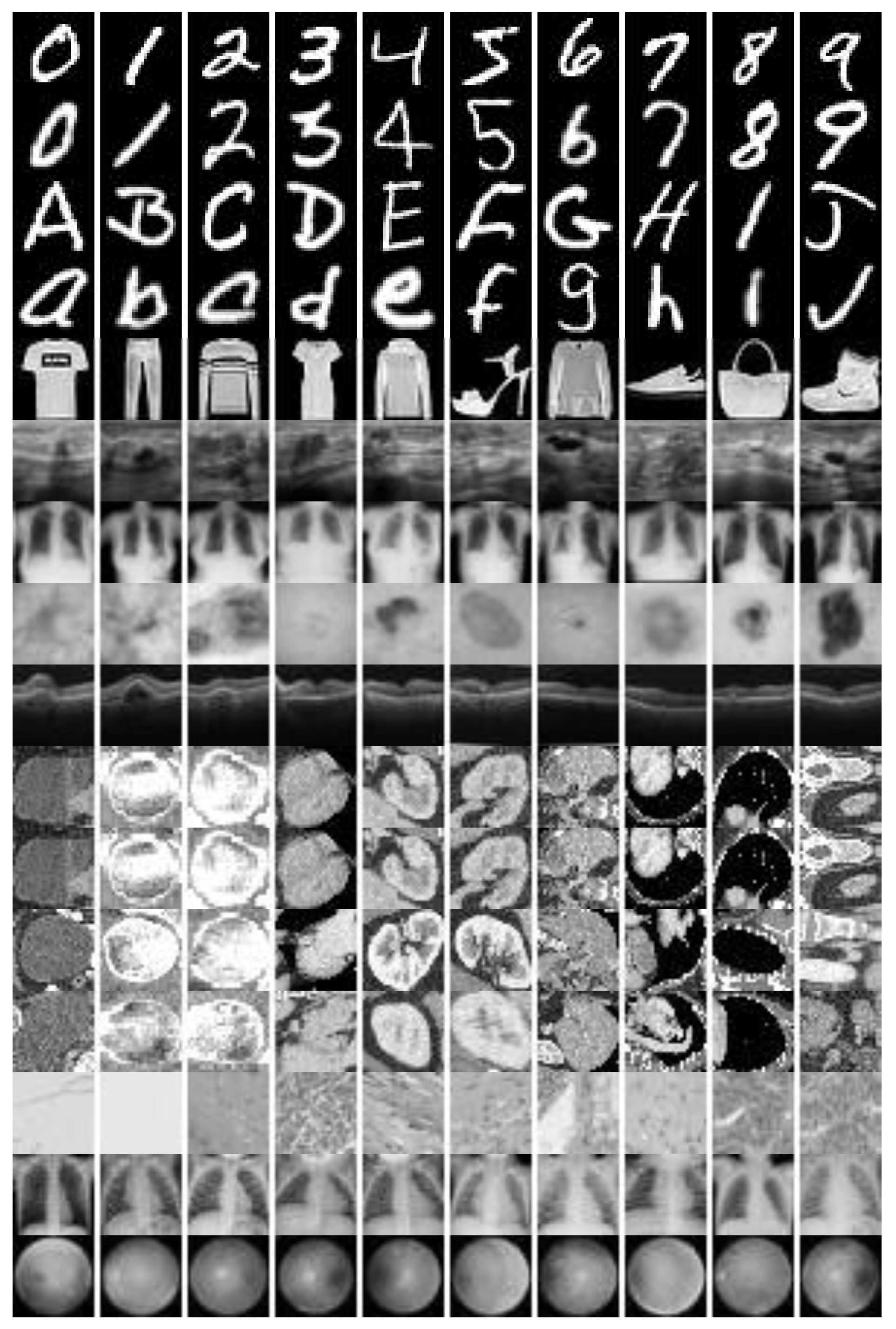
4.1. Experimental Data Sets
4.2. Experimental Conditions
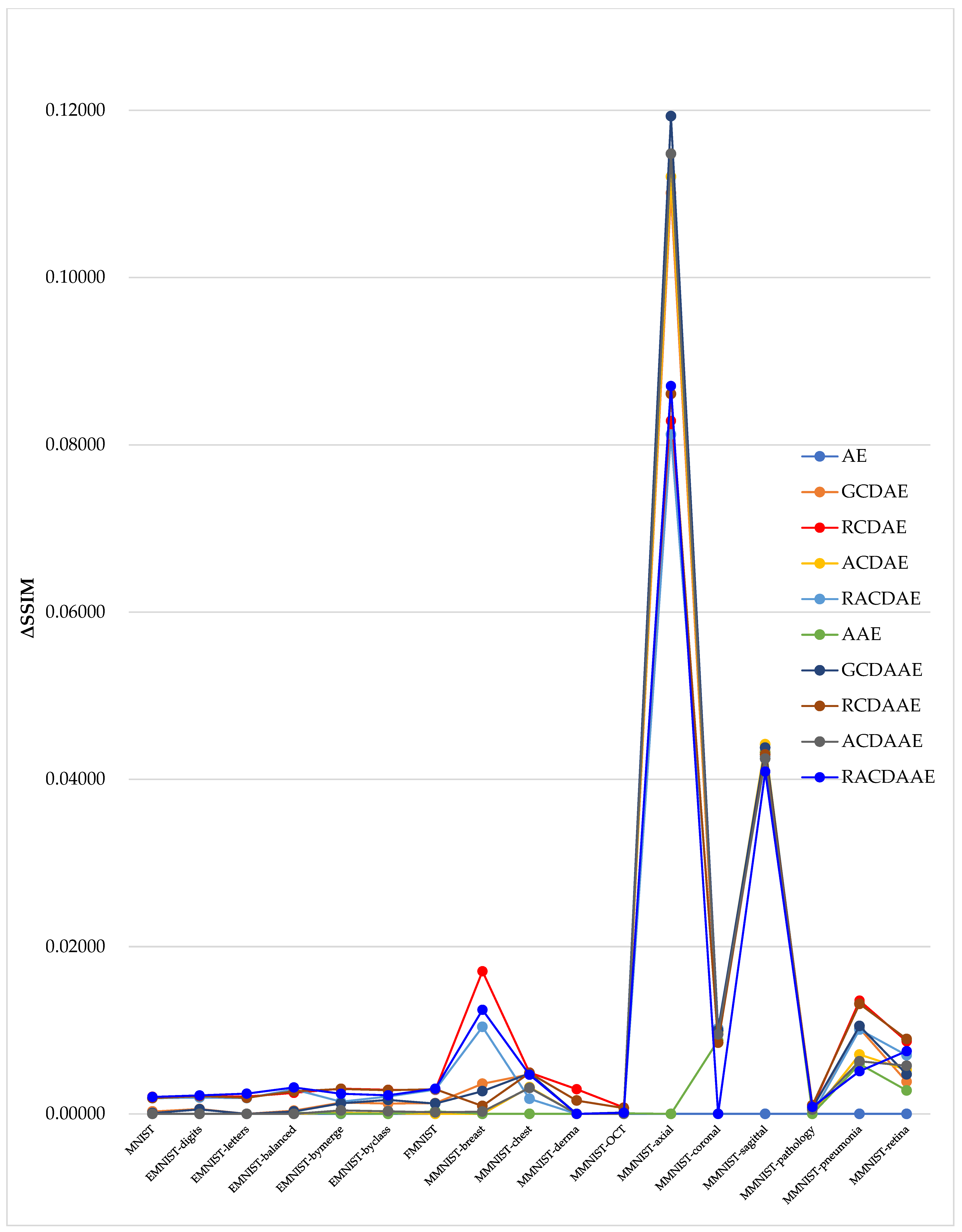
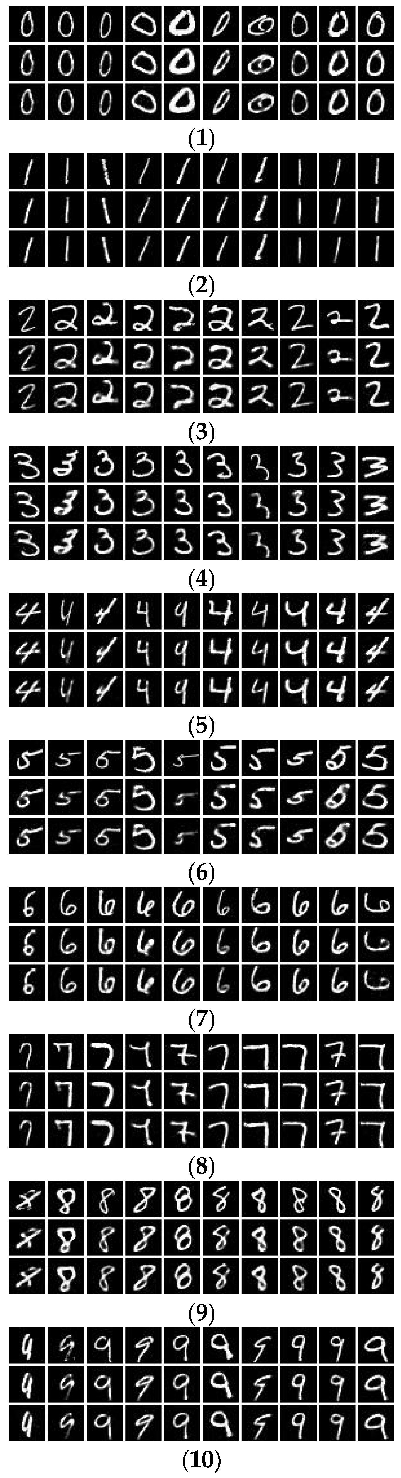
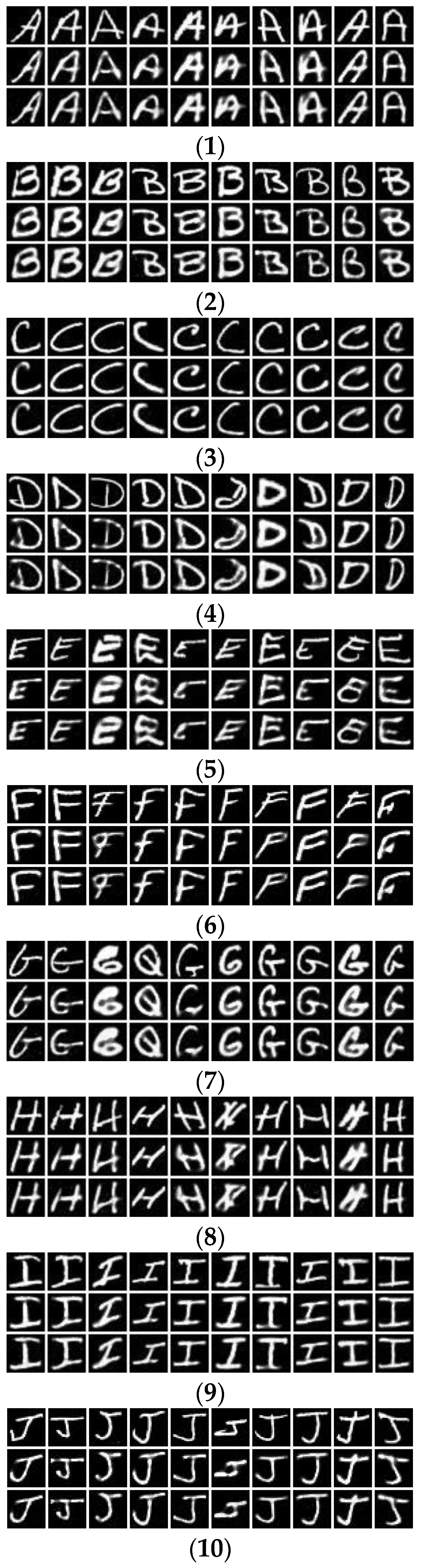
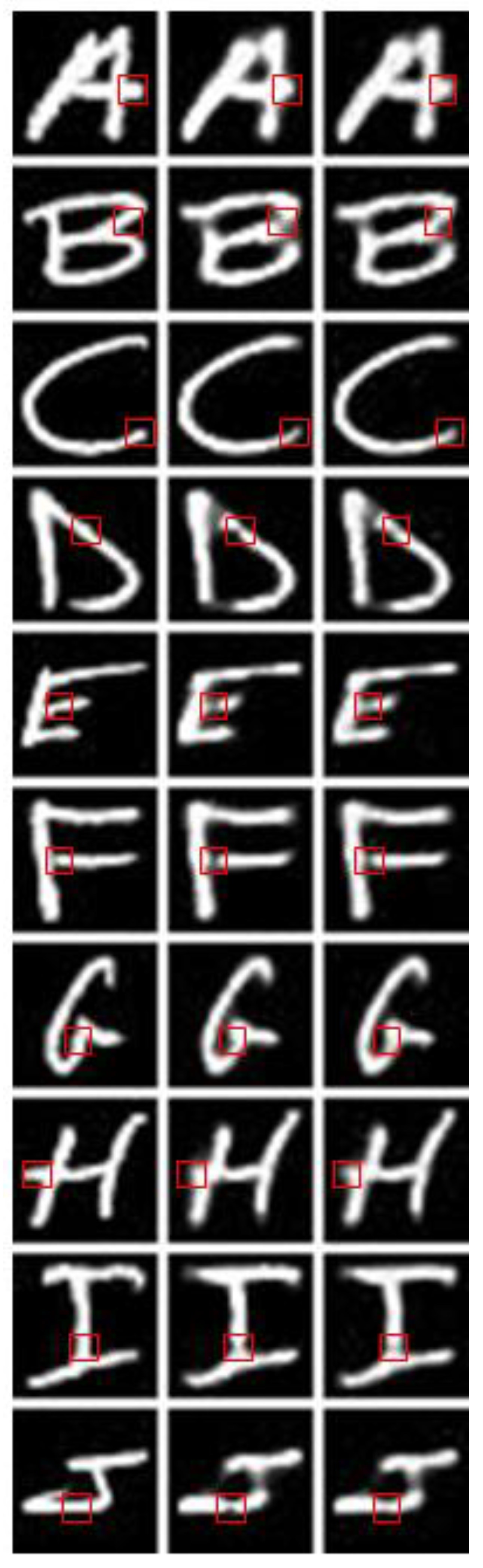
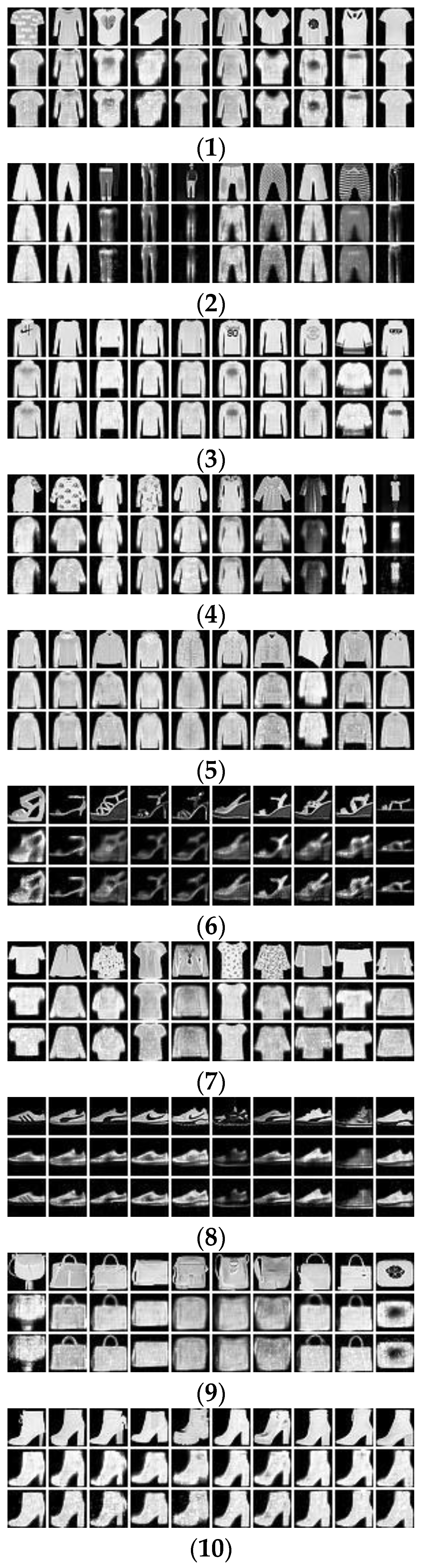
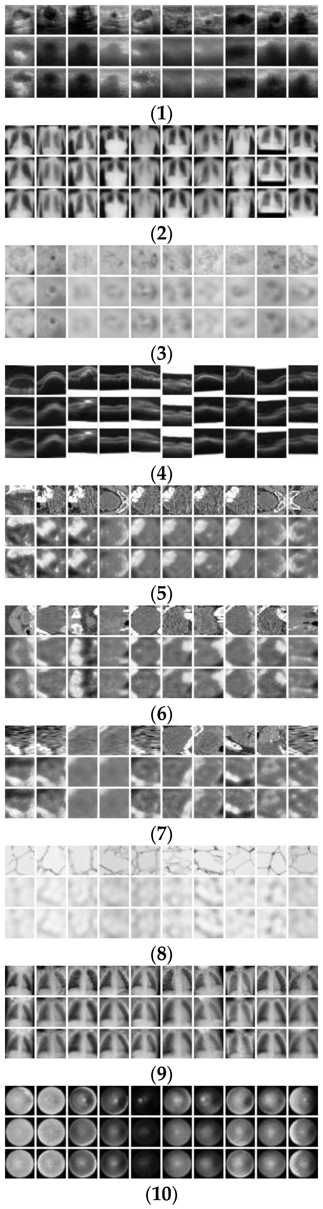
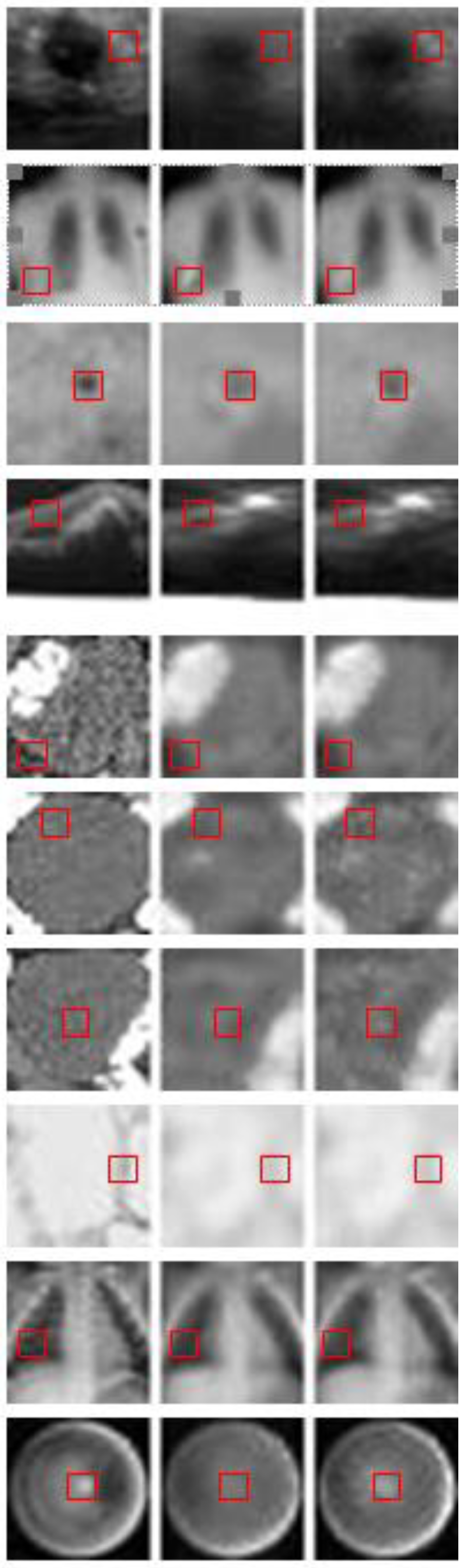
4.3. Experimental Results
5. Conclusions
6. Patents
Author Contributions
Funding
Institutional Review Board Statement
Informed Consent Statement
Data Availability Statement
Acknowledgments
Conflicts of Interest
References
- Zhang, Q.; Yang, L.T.; Chen, Z.; Li, P. A survey on deep learning for big data. Inf. Fusion 2018, 42, 146–157. [Google Scholar] [CrossRef]
- Grant, W.H.; Wei, Y. A survey of deep learning: Platforms, applications and emerging research trends. IEEE Access 2018, 6, 24411–24432. [Google Scholar]
- Dong, G.G.; Liao, G.S.; Liu, H.W.; Kuang, G.Y. A Review of the autoencoder and its variants: A comparative perspective from target recognition in synthetic-aperture radar images. IEEE Geosci. Remote Sens. Mag. 2018, 6, 44–68. [Google Scholar] [CrossRef]
- Doersch, C. Tutorial on variational autoencoders. arXiv 2016, arXiv:1606.05908. [Google Scholar]
- Kingma, P.D.; Welling, M. Auto-encoding variational Bayes. arXiv 2014, arXiv:1312.6114. [Google Scholar]
- Angshul, M. Blind denoising autoencoder. IEEE Trans. Neural Netw. Learn. Syst. 2019, 30, 312–317. [Google Scholar]
- Wu, T.; Zhao, W.F.; Keefer, E.; Zhi, Y. Deep compressive autoencoder for action potential compression in large-scale neural recording. J. Neural Eng. 2018, 15, 066019. [Google Scholar] [CrossRef] [PubMed]
- Anupriya, G.; Angshul, M.; Rabab, W. Semi-supervised stacked label consistent autoencoder for reconstruction and analysis of biomedical signals. IEEE Trans. Biomed. Eng. 2017, 64, 2196–2205. [Google Scholar]
- Toderici, G.; O’Malley, M.S.; Hwang, S.J.; Vincent, D.; Minnen, D.; Baluja, S.; Covell, M.; Sukthankar, R. Variable rate image compression with recurrent neural networks. In Proceedings of the 4th International Conference of Learning Representations (ICLR2016), San Juan, Puerto Rico, 2–4 May 2016. [Google Scholar]
- Rippel, O.; Nair, S.; Lew, C.; Branson, S.; Anderson, G.A.; Bourdevar, L. Learned video compression. arXiv 2018, arXiv:1811.06981. [Google Scholar]
- Makhzani, A.; Shlens, J.; Jaitly, N.; Goodfellow, I.; Frey, B. Adversarial autoencoders. arXiv 2016, arXiv:1511.05644v2. [Google Scholar]
- Ozal, Y.; Ru, T.S.; Rajendra, U.A. An efficient compression of ECG signals using deep convolutional autoencoders. Cogn. Syst. Res. 2018, 52, 198–211. [Google Scholar]
- Jonathan, R.; Jonathan, P.O.; Alan, A.G. Quantum autoencoders for efficient compression of quantum data. Quantum Sci. Technol. 2017, 2, 045001. [Google Scholar]
- Han, T.; Hao, K.R.; Ding, Y.S.; Tang, X.S. A sparse autoencoder compressed sensing method for acquiring the pressure array information of clothing. Neurocomputing 2018, 275, 1500–1510. [Google Scholar] [CrossRef]
- Tolstikhin, I.; Bousquet, O.; Gelly, S.; Schoelkopf, B. Wasserstein auto-encoders. In Proceedings of the 6th International Conference of Learning Representations (ICLR2018), Vancouver, BC, Canada, 30 April–3 May 2018. [Google Scholar]
- Angshul, M. Graph structured autoencoder. Neural Netw. 2018, 106, 271–280. [Google Scholar]
- Li, H.G. Deep linear autoencoder and patch clustering based unified 1D coding of image and video. J. Electron. Imaging 2017, 26, 053016. [Google Scholar] [CrossRef]
- Li, H.G.; Trocan, M. Deep residual learning-based reconstruction of stacked autoencoder representation. In Proceedings of the 25th IEEE International Conference on Electronics, Circuits and Systems (ICECS2018), Bordeaux, France, 9–12 December 2018. [Google Scholar]
- Perera, P.L.; Mo, B. Ship performance and navigation data compression and communication under autoencoder system architecture. J. Ocean Eng. Sci. 2018, 3, 133–143. [Google Scholar] [CrossRef]
- Sun, B.; Feng, H. Efficient compressed sensing for wireless neural recording: A deep learning approach. IEEE Signal Proc. Lett. 2017, 24, 863–867. [Google Scholar] [CrossRef]
- Angshul, M. An autoencoder based formulation for compressed sensing reconstruction. Magn. Reson. Imaging 2018, 52, 62–68. [Google Scholar]
- Yang, Y.M.; Wu, Q.M.J.; Wang, Y.N. Autoencoder with invertible functions for dimension reduction and image reconstruction. IEEE Trans. Syst. Man Cybern. Syst. 2018, 48, 1065–1079. [Google Scholar] [CrossRef]
- Majid, S.; Fardin, A.M. A deep learning-based compression algorithm for 9-DOF inertial measurement unit signals along with an error compensating mechanism. IEEE Sens. J. 2019, 19, 632–640. [Google Scholar]
- Cho, S.H. A technical analysis on deep learning based image and video compression. J. Broadcast Eng. 2018, 23, 383–394. [Google Scholar]
- Li, J.H.; Li, B.; Xu, J.Z.; Xiong, R.Q.; Gao, W. Fully connected network-based intra prediction for image coding. IEEE Trans. Image Proc. 2018, 27, 3236–3247. [Google Scholar] [CrossRef] [PubMed]
- Lu, G.; Ouyang, W.L.; Xu, D.; Zhang, X.Y.; Cai, C.L.; Gao, Z.Y. DVC: An end-to-end deep video compression framework. arXiv 2018, arXiv:1812.00101. [Google Scholar]
- Cui, W.X.; Jiang, F.; Gao, X.W.; Tao, W.; Zhao, D.B. Deep neural network based sparse measurement matrix for image compressed sensing. arXiv 2018, arXiv:1806.07026. [Google Scholar]
- Karras, T.; Aila, T.; Laine, S.; Lehtinen, J. Progressive growing of GANs for improved quality, stability, and variation. In Proceedings of the 6th International Conference of Learning Representations (ICLR2018), Vancouver, BC, Canada, 30 April–3 May 2018. [Google Scholar]
- LeCun, Y.; Bottou, L.; Bengio, Y.; Haffner, P. Gradient-based learning applied to document recognition. Proc. IEEE 1998, 86, 2278–2324. [Google Scholar] [CrossRef]
- Gregory, C.; Saeed, A.; Jonathan, T.; Andre, S.V. EMNIST: Extending MNIST to handwritten letters. In Proceedings of the IEEE International Joint Conference on Neural Networks (IJCNN), Anchorage, AK, USA, 14–19 May 2017; pp. 2921–2926. [Google Scholar]
- Xiao, H.; Rasul, K.; Vollgraf, R. Fashion-MNIST: A novel image dataset for benchmarking machine learning algorithms. arXiv 2017, arXiv:1708.07747. [Google Scholar]
- Yang, J.C.; Shi, R.; Ni, B.B. MedMNIST classification decathlon: A lightweight AutoML benchmark for medical image analysis. arXiv 2020, arXiv:2010.14925. [Google Scholar]


| Auto-Encoders | References |
|---|---|
| Variational auto-encoders | [4] |
| Adversarial auto-encoders | [11] |
| Convolutional auto-encoders | [12] |
| Quantum auto-encoders | [13] |
| Sparse auto-encoders | [14] |
| Wasserstein auto-encoders | [15] |
| Graphical auto-encoders | [16] |
| Notations and Abbreviations | Meanings |
|---|---|
| AE | auto-encoders |
| AAE/VAE/WAE | adversarial/variational/Wasserstein AE |
| CD | cascade decoders |
| GCD/RCD/ACD/RACD | general/residual/adversarial/residual-adversarial CD |
| CD/GCDAE/RCDAE/ACDAE/RACDAE | CD/GCD/RCD/ACD/RACD-based AE |
| CDAAE/GCDAAE/RCDAAE/ACDAAE/RACDAAE | CD/GCD/RCD/ACD/RACD-based AAE |
| CDVAE/GCDVAE/RCDVAE/ACDVAE/RACDVAE | CD/GCD/RCD/ACD/RACD-based VAE |
| CDWAE/GCDWAE/RCDWAE/ACDWAE/RACDWAE | CD/GCD/RCD/ACD/RACD-based WAE |
| E/D/DC | encoder/decoder/discriminator |
| x/y/z | original/reconstructed/latent sample |
| Data Set | Class Number | Sample Number | ||
|---|---|---|---|---|
| Training | Testing | |||
| MNIST | 10 | 60,000 | 10,000 | |
| EMINST | digits | 10 | 240,000 | 40,000 |
| letters | 26 | 124,800 | 20,800 | |
| balanced | 47 | 112,800 | 18,800 | |
| bymerge | 47 | 697,932 | 116,323 | |
| byclass | 62 | 697,932 | 116,323 | |
| FMNIST | 10 | 60,000 | 10,000 | |
| MMNIST | breast | 2 | 546 | 156 |
| chest | 2 | 78,468 | 22,433 | |
| derma | 7 | 7007 | 2005 | |
| OCT | 4 | 97,477 | 1000 | |
| axial organ | 11 | 34,581 | 17,778 | |
| coronal organ | 11 | 13,000 | 8268 | |
| sagittal organ | 11 | 13,940 | 8829 | |
| pathology | 9 | 89,996 | 7180 | |
| pneumonia | 2 | 4708 | 624 | |
| retina | 5 | 1080 | 400 | |
| Parameter Name | Parameter Value |
|---|---|
| Image size | 28 × 28 × 1 |
| Latent Dimension | 30 |
| Decoder Number | 3 |
| Batch size | 100 |
| Learning Rate | 0.0002 |
| Iteration Epoch | 100 |
| Algorithms | SSIM | ΔSSIM |
|---|---|---|
| AE | 0.97387 | 0.00000 |
| GCDAE | 0.97415 | 0.00028 |
| RCDAE | 0.97592 | 0.00205 |
| ACDAE | 0.97354 | −0.00033 |
| RACDAE | 0.97574 | 0.00187 |
| AAE | 0.97304 | −0.00083 |
| GCDAAE | 0.97397 | 0.00010 |
| RCDAAE | 0.97576 | 0.00189 |
| ACDAAE | 0.97381 | −0.00006 |
| RACDAAE | 0.97589 | 0.00202 |
| Algorithms | SSIM ΔSSIM | ||||
|---|---|---|---|---|---|
| EMNIST | |||||
| Digits | Letters | Balanced | Bymerge | Byclass | |
| AE | 0.98322 0.00000 | 0.97466 0.00000 | 0.97277 0.00000 | 0.98288 0.00000 | 0.98309 0.00000 |
| GCDAE | 0.98380 0.00058 | 0.97466 0.00000 | 0.97315 0.00038 | 0.98423 0.00135 | 0.98432 0.00123 |
| RCDAE | 0.98528 0.00206 | 0.97672 0.00206 | 0.97528 0.00251 | 0.98589 0.00301 | 0.98597 0.00288 |
| ACDAE | 0.98285 −0.00037 | 0.97391 −0.00075 | 0.97223 −0.00054 | 0.98300 0.00012 | 0.98314 0.00005 |
| RACDAE | 0.98517 0.00195 | 0.97654 0.00188 | 0.97570 0.00293 | 0.98433 0.00145 | 0.98517 0.00208 |
| AAE | 0.98304 −0.00018 | 0.97434 −0.00032 | 0.97291 0.00014 | 0.98291 0.00003 | 0.98284 −0.00025 |
| GCDAAE | 0.98375 0.00053 | 0.97451 −0.00015 | 0.97305 0.00028 | 0.98413 0.00125 | 0.98476 0.00167 |
| RCDAAE | 0.98534 0.00212 | 0.97659 0.00193 | 0.97546 0.00269 | 0.98586 0.00298 | 0.98592 0.00283 |
| ACDAAE | 0.98305 −0.00017 | 0.97410 −0.00056 | 0.97275 −0.00020 | 0.98329 0.00041 | 0.98340 0.00031 |
| RACDAAE | 0.98543 0.00221 | 0.97708 0.00242 | 0.97593 0.00316 | 0.98529 0.00241 | 0.98531 0.00222 |
| Algorithms | SSIM | ΔSSIM |
|---|---|---|
| AE | 0.96335 | 0.00000 |
| GCDAE | 0.96463 | 0.00128 |
| RCDAE | 0.96620 | 0.00285 |
| ACDAE | 0.96329 | −0.00006 |
| RACDAE | 0.96625 | 0.00290 |
| AAE | 0.96366 | 0.00031 |
| GCDAAE | 0.96458 | 0.00123 |
| RCDAAE | 0.96630 | 0.00295 |
| ACDAAE | 0.96353 | 0.00018 |
| RACDAAE | 0.96637 | 0.00302 |
| Algorithms | SSIM ΔSSIM | |||||||||
|---|---|---|---|---|---|---|---|---|---|---|
| MedMNIST | ||||||||||
| Breast | Chest | Derma | Oct | Axial | Coronal | Sagittal | Pathology | Pneumonia | Retina | |
| AE | 0.88868 0.00000 | 0.98363 0.00000 | 0.97103 0.00000 | 0.98851 0.00000 | 0.81806 0.00000 | 0.82470 0.00000 | 0.79883 0.00000 | 0.89644 0.00000 | 0.94760 0.00000 | 0.97366 0.00000 |
| GCDAE | 0.89228 0.00360 | 0.98836 0.00473 | 0.97103 0.00000 | 0.98856 0.00005 | 0.92817 0.11011 | 0.83320 0.00850 | 0.84211 0.04328 | 0.89720 0.00076 | 0.95782 0.01022 | 0.97751 0.00385 |
| RCDAE | 0.90574 0.01706 | 0.98857 0.00494 | 0.97396 0.00295 | 0.98927 0.00076 | 0.90092 0.08286 | 0.83467 0.00997 | 0.84180 0.04297 | 0.89724 0.00080 | 0.96115 0.01355 | 0.98233 0.00867 |
| ACDAE | 0.87883 −0.00985 | 0.98682 0.00319 | 0.96834 −0.00269 | 0.98780 −0.00071 | 0.93012 0.11206 | 0.83450 0.00980 | 0.84302 0.04419 | 0.89548 −0.00096 | 0.95469 0.00709 | 0.97892 0.00526 |
| RACDAE | 0.89908 0.01040 | 0.98543 0.00180 | 0.97028 −0.00075 | 0.98832 −0.00019 | 0.89931 0.08125 | 0.83494 0.01024 | 0.84155 0.04272 | 0.89594 −0.00050 | 0.95784 0.01008 | 0.98067 0.00701 |
| AAE | 0.88527 −0.00341 | 0.97240 −0.01230 | 0.97052 −0.00051 | 0.98858 0.00007 | 0.81498 −0.00308 | 0.83347 0.00877 | 0.84202 0.04319 | 0.89603 −0.00041 | 0.95356 0.00596 | 0.97646 0.00280 |
| GCDAAE | 0.89139 0.00271 | 0.98847 0.00484 | 0.97054 −0.00053 | 0.98867 0.00016 | 0.93736 0.11930 | 0.83347 0.01000 | 0.84261 0.04378 | 0.89714 0.00070 | 0.95811 0.01051 | 0.97839 0.00473 |
| RCDAAE | 0.89772 0.00094 | 0.98852 0.00489 | 0.97262 0.00159 | 0.98920 0.00069 | 0.89873 0.08607 | 0.83321 0.00851 | 0.84179 0.04296 | 0.89747 0.00103 | 0.96076 0.01316 | 0.98261 0.00895 |
| ACDAAE | 0.88895 0.00027 | 0.98673 0.00310 | 0.96987 −0.00116 | 0.98769 −0.00082 | 0.93286 0.11480 | 0.83421 0.00951 | 0.84129 0.04246 | 0.89695 0.00051 | 0.95389 0.00629 | 0.97942 0.00576 |
| RACDAAE | 0.90113 0.01245 | 0.98831 0.00468 | 0.97062 −0.00041 | 0.98865 0.00014 | 0.90580 0.08702 | 0.83380 −0.00090 | 0.83975 0.04092 | 0.89728 0.00084 | 0.95720 0.00510 | 0.98117 0.00751 |
Publisher’s Note: MDPI stays neutral with regard to jurisdictional claims in published maps and institutional affiliations. |
© 2022 by the authors. Licensee MDPI, Basel, Switzerland. This article is an open access article distributed under the terms and conditions of the Creative Commons Attribution (CC BY) license (https://creativecommons.org/licenses/by/4.0/).
Share and Cite
Li, H.; Trocan, M.; Sawan, M.; Galayko, D. Serial Decoders-Based Auto-Encoders for Image Reconstruction. Appl. Sci. 2022, 12, 8256. https://doi.org/10.3390/app12168256
Li H, Trocan M, Sawan M, Galayko D. Serial Decoders-Based Auto-Encoders for Image Reconstruction. Applied Sciences. 2022; 12(16):8256. https://doi.org/10.3390/app12168256
Chicago/Turabian StyleLi, Honggui, Maria Trocan, Mohamad Sawan, and Dimitri Galayko. 2022. "Serial Decoders-Based Auto-Encoders for Image Reconstruction" Applied Sciences 12, no. 16: 8256. https://doi.org/10.3390/app12168256
APA StyleLi, H., Trocan, M., Sawan, M., & Galayko, D. (2022). Serial Decoders-Based Auto-Encoders for Image Reconstruction. Applied Sciences, 12(16), 8256. https://doi.org/10.3390/app12168256