
A Fine-Grained Network Congestion Detection Based on Flow Watermarking

Abstract
:1. Introduction
- (1)
- Carrier: Indicating the detection method.
- (2)
- Whether to occupy extra bandwidth: Occupying extra bandwidth will cause the ‘observer effect’.
- (3)
- Whether to modify the packet content: Modifying the packet content will bring security problems and additional switch overhead.
- (4)
- Detection speed: Reacting to the efficiency of network congestion detection.
- First, we design a network congestion detection model based on flow watermarking and theoretically analyze the network congestion detection method based on flow watermarking. The flow watermarking is applied to network congestion detection for the first time, which doesn’t occupy extra bandwidth, change the payload of the packet, and increase the processing burden.
- Second, we propose a fine-grained network congestion detection algorithm to solve the problem that the congestion caused by micro-burst traffic has the characteristics of short duration and rapid change, which makes it difficult to detect by conventional congestion detection methods; it can detect network congestion on a small time scale and we can obtain current network status by analyzing the watermark decoding information.
- Third, we introduce eBPF into network congestion detection based on flow watermarking to enable it easy to employ. The experimental results show that the flow watermarking is sensitive to the changes in network status. The fine-grained network congestion detection algorithm can more accurately judge network status.
2. Related Work
2.1. Network Congestion Detection
2.2. Network Flow Watermarking
2.3. eBPF
3. Network Congestion Detection Model Based on Flow Watermarking
3.1. Congestion Detection Model Based on Watermark
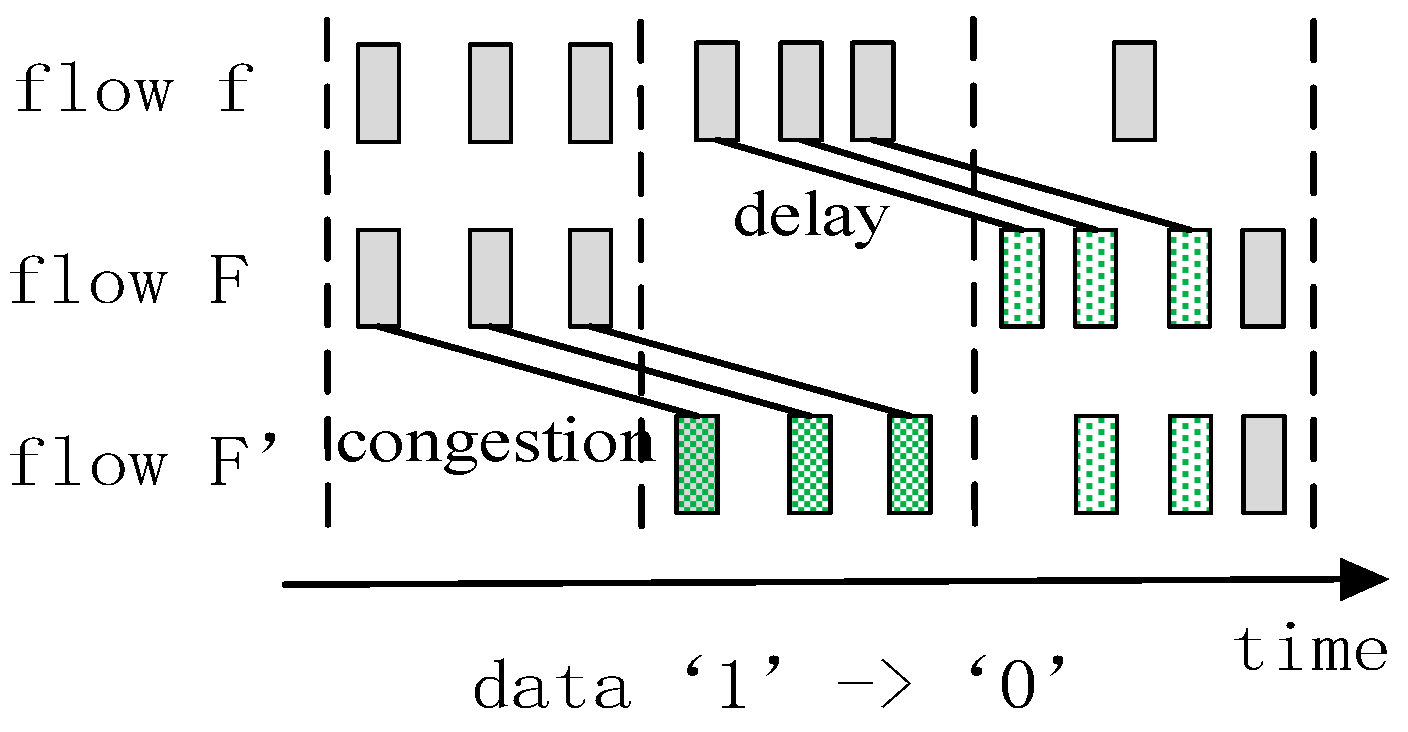
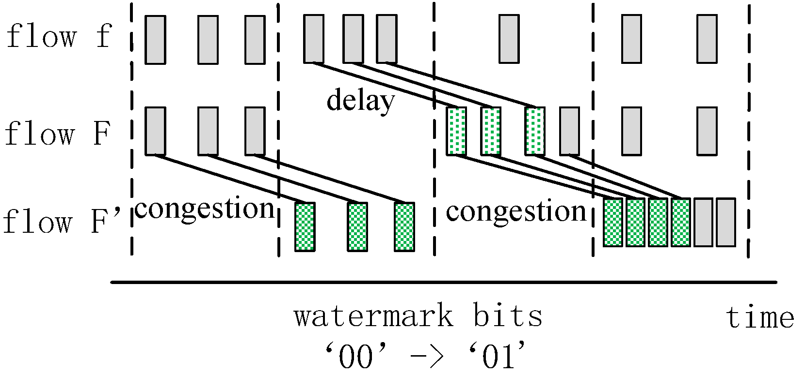
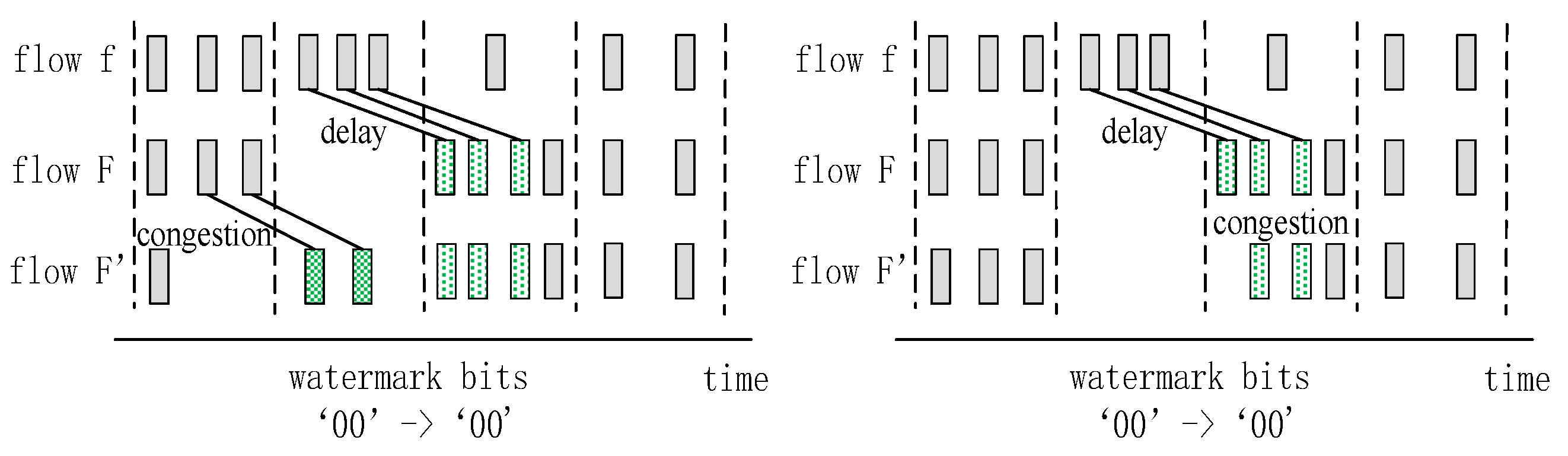
3.2. Watermark Mechanism Based on Sparsity of Packet
4. Theoretical Analysis of Network Congestion Detection Based on Flow Watermarking
4.1. Analysis of the SRW without Interference
4.2. Analysis of the SRW When Packet Delay Occurs
4.3. Analysis of the SRW When Packet Loss Occurs
5. Fine-Grained Network Congestion Detection Algorithm Based on Flow Watermarking
5.1. Analysis of SRW in Micro-Burst Traffic Model
5.2. Fine-Grained Network Congestion Detection Algorithm
6. Evaluation
6.1. Experiment Environment
6.2. Experiment Result and Analysis
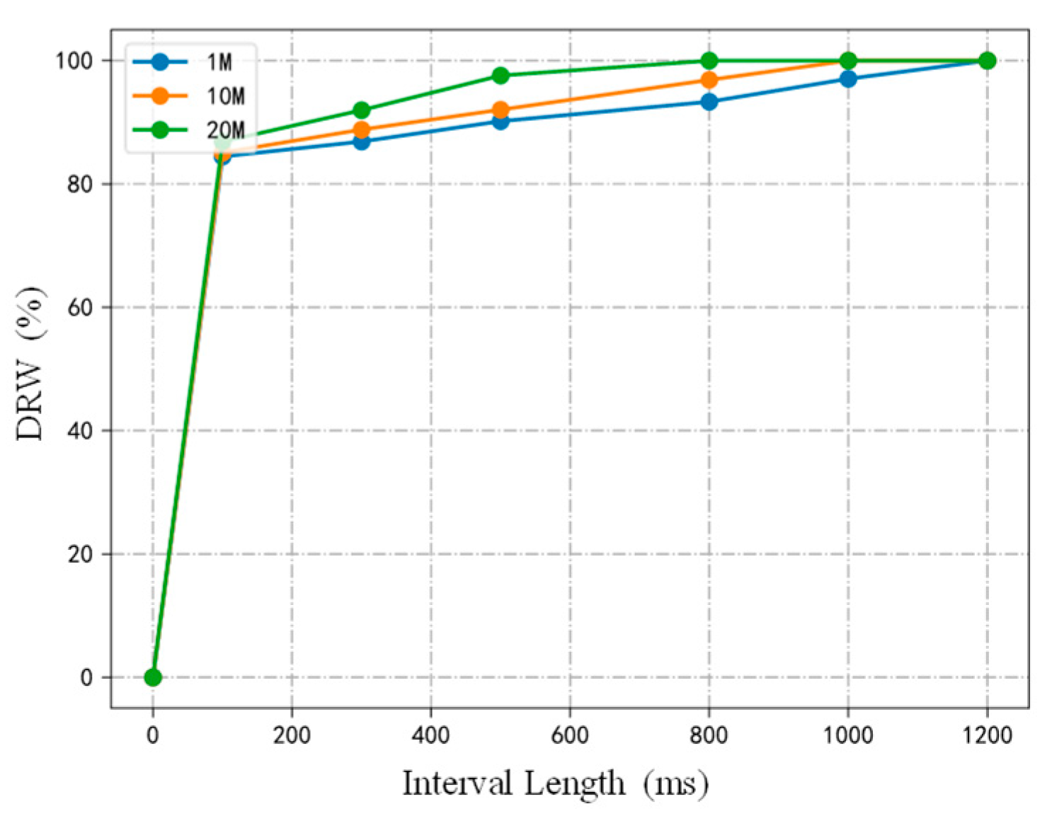
- (1)
- The increase of the length of interval and flow rate will improve DRW.
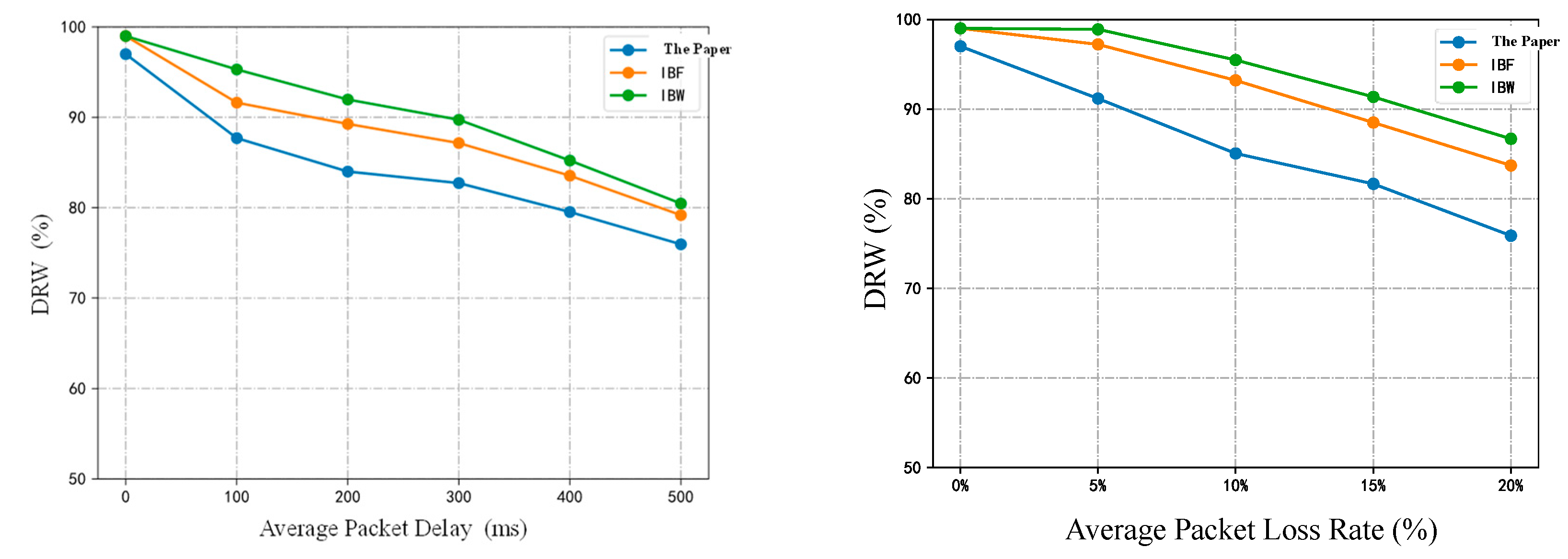
- (2)
- DRW in different packet delays and packet loss rates.
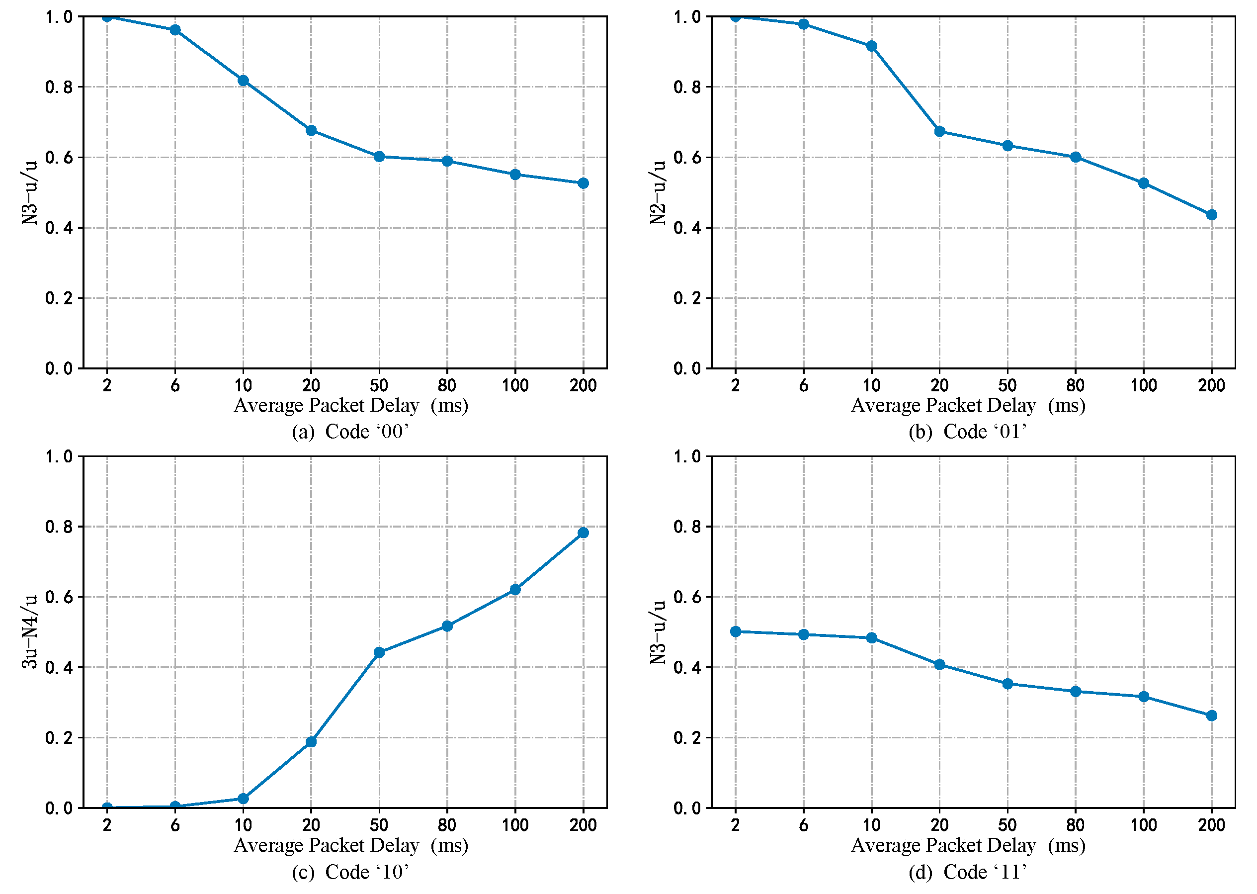
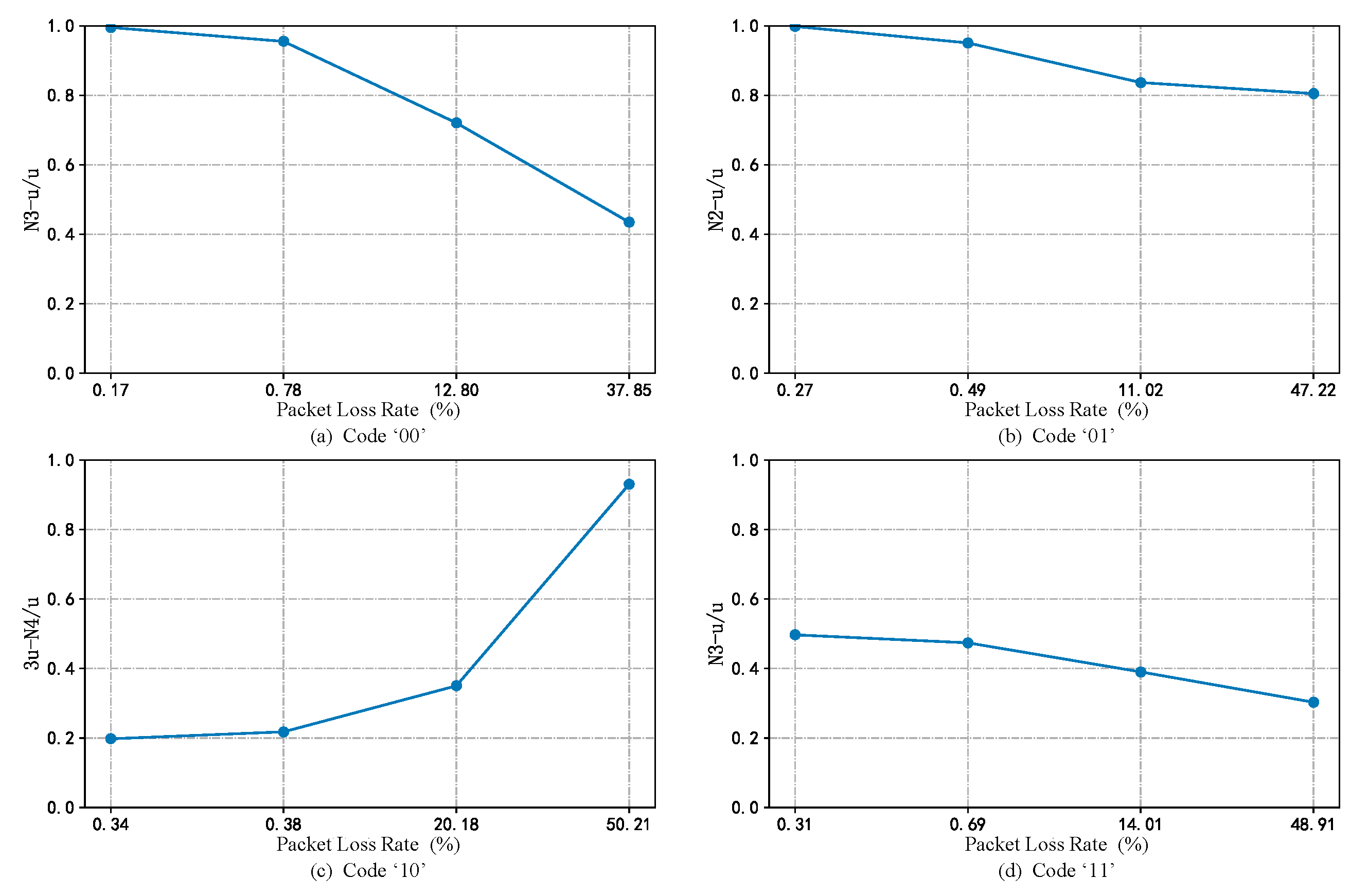
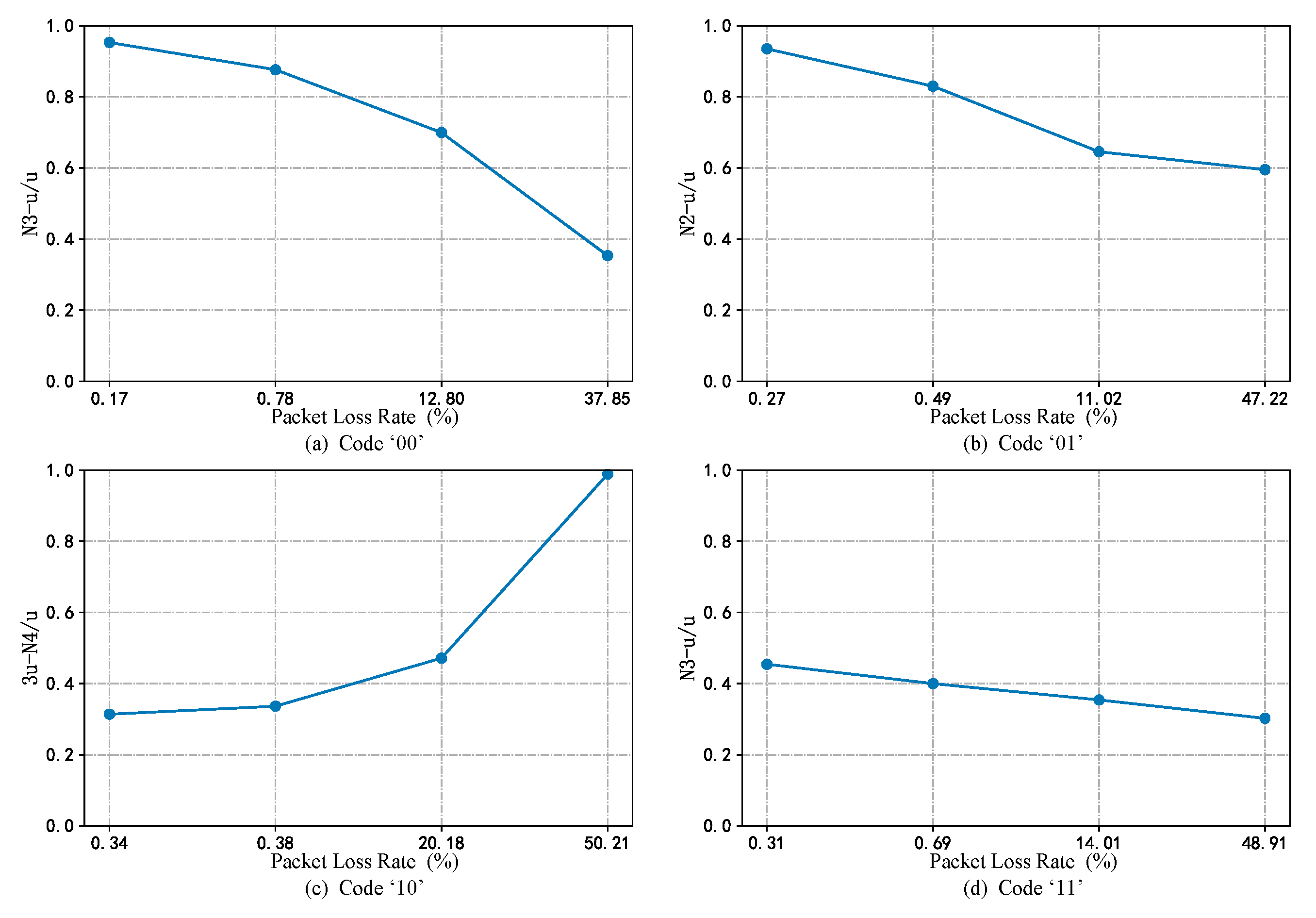
- (3)
- Evaluation of fine-grained network congestion detection algorithms in three scenes.
7. Conclusions and Further Work
Author Contributions
Funding
Institutional Review Board Statement
Informed Consent Statement
Data Availability Statement
Conflicts of Interest
References
- Huawei.AI Fabric, Intelligent and Lossless Data Center Network in the AI Era [DB/OL]. Available online: https://www.huawei.com/en/news/2018/12/huawei-releases-ai-fabric-white-paper (accessed on 20 December 2018).
- Zhang, L.; Kong, Y.; Guo, Y.; Yan, J.; Wang, Z. Survey on network flow watermarking: Model, interferences, applications, technologies and security. IET Commun. 2018, 12, 1639–1648. [Google Scholar] [CrossRef]
- Luo, Y. Research on Proactive Defense of Compute Network; CNKI: Beijing, China, 2017. [Google Scholar]
- Lin, C.; Han, G.; Du, J.; Xu, T.; Peng, Y. Adaptive traffic engineering based on active network measurement towards software defined internet of vehicles. IEEE Trans. Intell. Transp. Syst. 2020, 22, 3697–3706. [Google Scholar] [CrossRef]
- Liu, L.; Zhang, H.; Shi, J.; Yu, X.; Xu, H. I2P anonymous communication network measurement and analysis. In Proceedings of the International Conference on Smart Computing and Communication, Sarawak, Malaysia, 28–30 June 2019; Springer: Cham, Switzerland, 2019; pp. 105–115. [Google Scholar]
- Choi, A.; Karamollahi, M.; Williamson, C.; Arlitt, M. Zoom Session Quality: A Network-Level View. In Proceedings of the International Conference on Passive and Active Network Measurement, Virtual Event, 28–30 March 2022; Springer: Cham, Switzerland, 2022; pp. 555–572. [Google Scholar]
- Nayak, P.; Knightly, E.W. Virtual speed test: An ap tool for passive analysis of wireless lans. Comput. Commun. 2022, 192, 185–196. [Google Scholar] [CrossRef]
- Liu, C.; Ju, W.; Zhang, G.; Xu, X.; Tao, J.; Jiang, D.; Lu, J. A SDN-based active measurement method to traffic QoS sensing for smart network access. Wirel. Netw. 2021, 27, 3677–3688. [Google Scholar] [CrossRef]
- Shimokawa, S.; Taenaka, Y.; Tsukamoto, K.; Lee, M. Sdn based in-network two-staged video qoe estimation with measurement error correction for edge network. IEEE Access 2021, 9, 39733–39745. [Google Scholar] [CrossRef]
- Cai, W.; Song, X.; Liu, C.; Jiang, D.; Huo, L. An Adaptive and Efficient Network Traffic Measurement Method Based on SDN in IoT. In Proceedings of the International Conference on Simulation Tools and Techniques, Istanbul, Türkiye, 20–21 October 2022; Springer: Cham, Switzerland, 2022; pp. 64–74. [Google Scholar]
- Van Adrichem, N.L.M.; Doerr, C.; Kuipers, F.A. Opennetmon: Network monitoring in openflow software-defined networks. In Proceedings of the 2014 IEEE Network Operations and Management Symposium (NOMS), Krakow, Poland, 5–9 May 2014; pp. 1–8. [Google Scholar]
- Yu, C.; Lumezanu, C.; Sharma, A.; Xu, Q.; Jiang, G.; Madhyastha, H. Software-defined latency monitoring in data center networks. In Proceedings of the International Conference on Passive and Active Network Measurement, New York, NY, USA, 19–20 March 2015; Springer: Cham, Switzerland, 2015; pp. 360–372. [Google Scholar]
- Fu, C.; John, W.; Meirosu, C. Eple: An efficient passive lightweight estimator for sdn packet loss measurement. In Proceedings of the 2016 IEEE Conference on Network Function Virtualization and Software Defined Networks (NFV-SDN), Palo Alto, CA, USA, 7–10 November 2016; pp. 192–198. [Google Scholar]
- Li, Y.; Miao, R.; Liu, H.H.; Zhuang, Y.; Feng, F.; Tang, L.; Cao, Z.; Zhang, M.; Kelly, F.; Alizadeh, M.; et al. HPCC: High precision congestion control. In Proceedings of the ACM Special Interest Group on Data Communication (SIGCOMM’19), Beijing, China, 19–23 August 2019; Association for Computing Machinery: New York, NY, USA, 2019; pp. 44–58. [Google Scholar] [CrossRef]
- Cui, M.; Li, X.; Wang, Y.; Niu, T.; Yang, F. SPT: Sketch-based polling in-band network telemetry. In Proceedings of the MS 2022–2022 IEEE/IFIP Network Operations and Management Symposium, Budapest, Hungary, 25–29 April 2022; pp. 1–7. [Google Scholar]
- Pan, T.; Lin, X.; Song, H.; Song, E.; Bian, Z.; Li, H.; Zhang, J.; Li, F.; Huang, T.; Jia, C.; et al. INT-probe: Lightweight In-band Network-Wide Telemetry with Stationary Probes. In Proceedings of the 2021 IEEE 41st International Conference on Distributed Computing Systems (ICDCS), Washington, DC, USA, 7–10 July 2021; pp. 898–909. [Google Scholar]
- Zhu, Y.; Kang, N.; Cao, J.; Greenberg, A.; Lu, G.; Mahajan, R.; Maltz, D.; Yuan, L.; Zhang, M.; Zhao, B.Y.; et al. Packet-level telemetry in large datacenter networks. In Proceedings of the 2015 ACM Conference on Special Interest Group on Data Communication, London, UK, 17–21 August 2015; pp. 479–491. [Google Scholar]
- Katta, N.; Hira, M.; Kim, C.; Sivaraman, A.; Rexford, J. Hula: Scalable load balancing using programmable data planes. In Proceedings of the Symposium on SDN Research, Santa Clara, CA, USA, 14–15 March 2016; pp. 1–12. [Google Scholar]
- Pan, T.; Song, E.; Bian, Z.; Lin, X.; Peng, X.; Zhang, J.; Huang, T.; Liu, B.; Liu, Y. Int-path: Towards optimal path planning for in-band network-wide telemetry. In Proceedings of the IEEE INFOCOM 2019-IEEE Conference on Computer Communications, Paris, France, 29 April–2 May 2019; pp. 487–495. [Google Scholar]
- Iacovazzi, A.; Sarda, S.; Frassinelli, D.; Elovici, Y. Dropwat: An invisible network flow watermark for data exfiltration traceback. IEEE Trans. Inf. Forensics Secur. 2017, 13, 1139–1154. [Google Scholar] [CrossRef]
- Wang, X.; Reeves, D.S. Robust correlation of encrypted attack traffic through stepping stones by manipulation of interpacket delays. In Proceedings of the 10th ACM Conference on Computer and Communications Security, Washington, DC, USA, 27–30 October 2003; pp. 20–29. [Google Scholar]
- Houmansadr, A.; Kiyavash, N.; Borisov, N. RAINBOW: A Robust And Invisible Non-Blind Watermark for Network Flows. NDSS 2009, 47, 406–422. [Google Scholar]
- Yu, L.; Zhang, L.; Zhang, Y.; Wen, W.; Du, X.; Cao, F. Dynamic Interval-based Watermarking for Tracking down Network Attacks. In Proceedings of the 2021 IEEE 21st International Conference on Software Quality, Reliability and Security (QRS), Hainan, China, 6–10 December 2021; pp. 52–61. [Google Scholar]
- Yao, Z.; Zhang, L.; Ge, J.; Wu, Y.; Zhang, X. An Invisible Flow Watermarking for Traffic Tracking: A Hidden Markov Model Approach. In Proceedings of the ICC 2019–2019 IEEE International Conference on Communications (ICC), Shanghai, China, 20–24 May 2019; pp. 1–6. [Google Scholar]
- Wang, X.; Chen, S.; Jajodia, S. Network flow watermarking attack on low-latency anonymous communication systems. In Proceedings of the 2007 IEEE Symposium on Security and Privacy (SP’07), Oakland, CA, USA, 20–23 May 2007; pp. 116–130. [Google Scholar]
- Pyun, Y.J.; Park, Y.H.; Wang, X.; Reeves, D.S.; Ning, P. Tracing traffic through intermediate hosts that repacketize flows. In Proceedings of the IEEE INFOCOM 2007—26th IEEE International Conference on Computer Communications, Anchorage, AK, USA, 6–12 May 2007; pp. 634–642. [Google Scholar]
- Houmansadr, A.; Borisov, N. SWIRL: A Scalable Watermark to Detect Correlated Network Flows. In Proceedings of the Network and Distributed System Security Symposium, NDSS 2011, San Diego, CA, USA, 6–9 February 2011. [Google Scholar]
- Wang, X.; Reeves, D.S.; Wu, S.F.; Yuill, J. Sleepy watermark tracing: An active network-based intrusion response framework. In Proceedings of the IFIP International Information Security Conference, Copenhagen, Denmark, 29 July–3 August 2001; Springer: Boston, MA, USA, 2001; pp. 369–384. [Google Scholar]
- Ramsbrock, D.; Wang, X.; Jiang, X. A first step towards live botmaster traceback. In Proceedings of the International Workshop on Recent Advances in Intrusion Detection, Cambridge, MA, USA, 15–17 September 2008; Springer: Berlin/Heidelberg, Germany, 2008; pp. 59–77. [Google Scholar]
- Zhang, L.; Wang, Z.; Xu, J. Flow watermarking scheme based on packet reordering. J. Softw. 2011, 22, 17–26. [Google Scholar]
- Xu, X.; Zhang, L.; Yan, J. PN Code Diversification Based Spread Spectrum Flow Watermarking Technology. In Proceedings of the 2018 14th International Conference on Computational Intelligence and Security (CIS), Hangzhou, China, 16–19 November 2018; pp. 254–258. [Google Scholar]
- Shi, J.; Zhang, L.; Yin, S.; Liu, W.; Zhai, J.; Liu, G.; Dai, Y. A Comprehensive Analysis of Interval Based Network Flow Watermarking. In Proceedings of the International Conference on Cloud Computing and Security, Singapore, 29–31 October 2018; Springer: Cham, Switzerland, 2018; pp. 72–84. [Google Scholar]
- Abranches, M.; Michel, O.; Keller, E.; Schmid, S. Efficient Network Monitoring Applications in the Kernel with eBPF and XDP. In Proceedings of the 2021 IEEE Conference on Network Function Virtualization and Software Defined Networks (NFV-SDN), Heraklion, Greece, 9–11 November 2021; pp. 28–34. [Google Scholar]


| Classification | Carrier | Whether to Occupy Extra Bandwidth | Whether to Modify Packet Content | Detection Speed |
|---|---|---|---|---|
| Watermark-based detection | IPD | No | No | Fast |
| Active detection | Probe packets | Yes | No | Slow |
| Passive detection | Mirrored packets | No | No | Slow |
| SDN-based detection | Probe packets, etc. | Yes/No | No | Slower |
| INT-based detection | Packet header field | Yes/No | Yes | Fast |
| Classification | Example | Robustness | Invisibility | Coding Efficiency |
|---|---|---|---|---|
| Packet payload-based | SWT | ★★★ | ★ | ★★ |
| Traffic rate-based | PN-based SS | ★★ | ★ | ★ |
| Packet timing-based | IPD | ★ | ★ | ★★★ |
| RAINBOW | ★ | ★★ | ★★★ | |
| Packet interval-based | ICBW | ★★ | ★ | ★ |
| IBW | ★★ | ★ | ★ | |
| IBF | ★★ | ★★ | ★★ | |
| SWIRL | ★★ | ★★ | ★ | |
| Packet length-based | LBW | ★★★ | ★ | ★★★ |
| Packet order-based | PROFW | ★★★ | ★★★ | ★★ |
Publisher’s Note: MDPI stays neutral with regard to jurisdictional claims in published maps and institutional affiliations. |
© 2022 by the authors. Licensee MDPI, Basel, Switzerland. This article is an open access article distributed under the terms and conditions of the Creative Commons Attribution (CC BY) license (https://creativecommons.org/licenses/by/4.0/).
Share and Cite
Mo, L.; Lv, G.; Wang, B. A Fine-Grained Network Congestion Detection Based on Flow Watermarking. Appl. Sci. 2022, 12, 8094. https://doi.org/10.3390/app12168094
Mo L, Lv G, Wang B. A Fine-Grained Network Congestion Detection Based on Flow Watermarking. Applied Sciences. 2022; 12(16):8094. https://doi.org/10.3390/app12168094
Chicago/Turabian StyleMo, Lusha, Gaofeng Lv, and Baosheng Wang. 2022. "A Fine-Grained Network Congestion Detection Based on Flow Watermarking" Applied Sciences 12, no. 16: 8094. https://doi.org/10.3390/app12168094
APA StyleMo, L., Lv, G., & Wang, B. (2022). A Fine-Grained Network Congestion Detection Based on Flow Watermarking. Applied Sciences, 12(16), 8094. https://doi.org/10.3390/app12168094