Abstract
The measurement of the shear wave velocities (Vs) of soils is an important aspect of geotechnical and earthquake engineering, due to its direct relation to the shear modulus (G), which in turn influences the stress–strain behavior of geomaterials. Vs can be directly measured or estimated using a variety of onsite tests or in a laboratory. Methods such as downhole PS logging require boreholes and may not be logistically and economically feasible in all situations. Many researchers have estimated Vs from other geotechnical parameters, such as standard penetration test resistance (SPT-N), by means of empirical correlations. This paper aimed to contribute to this subject by developing an empirical relationship between Vs and SPT-N. Data from twenty sites in Metro Manila were obtained from geotechnical investigation reports. Vs profiles of the same sites were also acquired using the refraction microtremor method. New empirical relationships were developed for all, sandy, and clayey soil types, using a non-linear regression method that is applicable for Metro Manila soils. Statistical evaluation and comparison of the proposed correlations with other previous works suggested the viability of the empirical model.
1. Introduction
The measurement of the shear wave velocities (Vs) of soils is an important aspect in the application of geotechnical and earthquake engineering. This geophysical parameter is related to the shear modulus (G) through the elastic theory, in the equation G = ρVs2, where ρ is the density of material. The stress–strain behavior of materials is then dictated by the shear modulus, as the strain is directly affected by this parameter [1]. This relationship is also important in ground response analysis, as it is used to evaluate the dynamic response of soils during earthquakes. The seismic shear wave velocity of the upper 30-m soil layer (Vs30) largely influences the ground motion amplification and is therefore considered an important parameter in earthquake engineering [2]. Additionally, the shear wave velocity of geomaterials is also used in studies on soil stratigraphy, liquefaction analysis, and site-specific subsurface modeling [3,4,5].
Shear wave velocities can be measured or estimated using a variety of laboratory or field tests. Bender element and resonant columns are some of the laboratory techniques that measure Vs. The accuracy of these techniques is greatly dependent on the degree of disturbance of the soil samples [6]. In situ field measurements include invasive methods such as down-hole, cross-hole, and up-hole tests. These techniques require the drilling of boreholes to a particular depth and, thus, may not be economically feasible in all situations. On the other hand, non-invasive geophysical methods, such as spectral analysis of surface waves (SASW), multichannel analysis of surface waves (MASW), refraction microtremor (ReMi), among others, can also estimate Vs on site. These techniques do not require drilling equipment and only use acoustic sensors to determine the subsurface shear wave velocities.
There have been attempts to correlate this geophysical parameter to other physically measured soil properties. These empirical correlations between the geotechnical parameters of soil and Vs were established in order to aid in soil behavior estimation and seismic demand analysis (e.g., Azam Ghazi et al., 2015 [7]; Gautam, 2017 [2]). However, these relationships are only accepted in localized data. In Japan, many works regarding this area were done in the 1970s, utilizing datasets from different regions (i.e., Imai and Yoshimura, 1970 [8]; Ohba and Toriumi, 1970 [9]; Shibata, 1970 [10]; Ohta et al., 1972 [11]; Fujiwara, 1972 [12]; Ohsaki and Iwasaki, 1973 [13]; Imai, 1977 [14]). These works mainly evaluated the dynamic response of soils (e.g., liquefaction) due to earthquakes. This continued into the 1980s, as Imai and Tonouchi (1982) [15] proposed a correlation with the most data points (n = 1654) based on the relative density of the subsurface soil (N-value), soil type, and geologic age. The work of Imai and Tonouchi (1982) also indicated that clayey layers have higher Vs values in comparison to sandy soils. In the United States, a similar correlation was proposed by Seed and Idriss (1981) [16], to determine liquefaction susceptibility of alluvium and marine sands. Their correlation utilizes corrected SPT parameters such as the N60 and (N1)60. This proposal is similar with the works by Seed et al., (1985) [17]; Sykora and Stokoe (1983) [18], Rollins et al. (1998) [19], and Brandenberg et al., (2010) [20].
Other countries have developed similar empirical correlations. Over the past decades, works by Kalteziotis et al. (1992) [21], Pitilakis et al. (1999) [22], Athanasopoulos (1995) [23], Raptakis et al. (1995) [24], Tsiambaos and Sabatakakis (2011) [25] have been completed in Greece. From Turkey, works by Iyisan (1996) [26], Kayabali (1996) [27], Hasancebi and Ulusay (2007) [28], Koçkar and Akgün (2008) [29], Dikmen (2009) [30], and Akin et al. (2011) [31] also explored the empirical correlations between Vs and SPT-N values and other geotechnical parameters. A considerable number of works on this topic have also been done in India: Anbazhagan and Sitharam (2010) [32], Anbazhagan et al. (2013) [33], Hanumantharao and Ramana (2008) [34], and Uma Maheswari et al. (2010) [35]. Kuo et al. (2011) [36] correlated Vs in terms of soil characteristics such as depth, soil type, and SPT-N value, using datasets from Taiwan.
Due to differences in soil type and properties from region to region, which arise from differences in geologic settings and active geomorphic processes, the proposed empirical correlations are local and were only extrapolated to areas with a similar lithology. The application was generally constrained to similar soil conditions and geomorphic settings. As such, despite the numerous proposed empirical correlations, there is still a great importance in correlating Vs and geotechnical parameters using datasets from local settings. Additionally, a variety of reasons, such as lack of drilling and geophysical equipment, personnel, and/or budget, can hinder the carrying out of downhole measurements of Vs, especially in smaller projects in the Philippines. Direct Vs measurements may be preferable, but in most cases where this is not feasible, empirical correlations between Vs and geotechnical parameters can be useful for site investigations.
The main objective of this paper was to develop an empirical relationship between Vs values from a refraction microtremor to N-values from standard penetration test drillings, using statistical regression analysis. Twenty sites (20) in Metro Manila, Philippines were surveyed using the refraction microtremor technique to establish one-dimensional Vs profiles correlated to N-values from SPT. The proposed empirical relationship between Vs and the N-value of soils in Metro Manila represents an important development in site characterization techniques and seismic microzonation efforts in the study area.
2. The Study Area
Metropolitan Manila (Metro Manila) is the capital region of the Philippines (Figure 1), which is also the center of the economy and the most populated areas. The region is composed of several cities and municipalities, sprawled over an area of around 620 square kilometers. It lies in the southern extension of the Luzon Central Valley. In the early stages of the development of the Central Valley, rapid sedimentation from highlands persisted until the Late Cretaceous, intercalated with tuff and other volcanic products [37]. During the Late Tertiary and Quaternary periods, complex tectonic events led to the basic geologic structure of Metro Manila at present. This geologic evolution has produced three distinct terranes in the metropolis: the Coastal Lowland, Central Plateau, and the Marikina Valley. East of the metropolis, the uplands of Rizal province with basement-ophiolite complexes can be found. To the west, this region is bounded by Manila Bay.
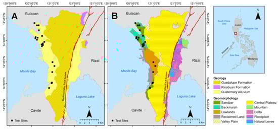
Figure 1.
(A) Geological and (B) geomorphologic map of Metro Manila, Philippines, and the locations of the refraction microtremor surveys. Geologic map modified from BMG (1983) [38] and geomorphologic map obtained from MMIERS (2004) [39]. Locations of the testing sites are also depicted in black squares.
The Coastal Lowland is the flat and low plain section of Metro Manila, facing the Manila Bay. This section can be further subdivided into deposits from sand bars, backmarshes, tidal flats, the Pasig River delta, and some reclaimed land. This Quaternary Alluvium deposit has a thickness that can reach up to 40 m [40]. Sixty percent of the Metro Manila area is underlain by the Central Plateau, which is the geomorphic manifestation of the bedrock of the region, namely the Diliman Tuff member of the Pleistocene Guadalupe Formation. This lithologic member is made of flat-lying sequences of medium to thin-bedded, fine-grained vitric tuff and welded pyroclastic breccias. Minor fine to medium-grained tuffaceous sandstone was also reported to be part of this unit [41]. The Marikina Valley is the flat section on the eastern bounds of the metropolis, with lower elevations than the Central Plateau. This is produced by a pull-apart basin associated with the West Valley Fault (WVF) and East Valley Fault (EVF), collectively called the Marikina Valley Fault System [42]. Quaternary alluvium deposits in this section are associated with the floodplain of the Marikina River and the delta along the Laguna de Bay. Surface deposits on this sector are reported to reach up to 50 m in thickness [40].
Geologic field mapping and different subsurface investigations have revealed that most of the Metro Manila soils and sediments are composed of thick sequences of pyroclastic and epiclastic deposits. Pyroclastic deposits, primarily tuff materials, are derived from eruptions of nearby volcanoes in the region. The epiclastic deposits come from pyroclastic materials that were reworked by fluvial and lacustrine processes. Tan (1983) [43] reported that these epiclastic fluvial deposits are generally made of a sequence of loose to firm silty fine sand at the surface, underlain by very soft clayey silt or silty clay, further underlain by stiff to very stiff clay, and finally hard clay and silt, sometimes intercalated with very dense sand and/or gravel that grade into bedrock. The thickness and lateral continuity of these layers is highly variable, such that during borehole investigations on a particular site, it is normal to encounter different thicknesses and sequences of soil and sediment deposits.
3. Field Investigations
3.1. Geotechnical Investigations
The most common type of geotechnical site investigation in the country is through the standard penetration test (SPT). The National Structural Code of the Philippines [44] requires at least one borehole for two-story structures and greater, with the number of boreholes determined depending on the footprint area of the building. This in situ geotechnical test involves the driving of a hollow tube into the soil, while noting the number of blows needed to push the tube sampler down a specific vertical distance. A 63.5 kg hammer is repeatedly dropped from a height of 76 cm to advance the tube, in three successive increments of 150 mm. The first 150 mm is considered as a seating penetration and is disregarded, while the total number of blows needed to penetrate the second and third 150-mm iterations is the determined N-value of that layer. This procedure is described in the ASTM D1586 [45] guideline. The number of blow counts or N-value can be affected by a variety of factors. The most important factors include the amount of energy delivered to the tube in each impact of the hammer, the type of hammer, diameter of the borehole, and the length of the rod.
Standard penetration test reports of twenty sites in Metro Manila (Figure 1) were obtained from the Department of Education, and Department of Public Works and Highways of the Philippines. These SPT investigations were typically carried out as a prerequisite before the construction of school buildings and other structures. The sites selected to be included in this study were identified as having sufficient space, where geophysical surveys can be conducted and geotechnical data are available. Moreover, the spatial distribution was intended so that there are representatives of the various major geomorphic units identified in the coastal portion of the area. These sites are located along the western coast of Metro Manila, atop the Coastal Lowlands, and are expected to have relatively thick soil deposits. Specifically, the sites were built on top of sandbars, backmarshes, and lowland deposits.
Most of the boreholes have depths that reach up to 15 m, the typical depth requirement for low-story buildings in the country. In some cases, the depth can reach up to 30 m, particularly for sites with thicker soil profiles. On the other hand, there are also SPT investigations where the penetration only reaches up to five to ten meters, for sites with a shallower bedrock depth. In such cases, a coring procedure is employed to penetrate the target depth. The obtained soil samples from the SPT investigation were subjected to typical laboratory tests, such as grain size analysis, moisture content determination, Atterberg Limit test, soil classification, and unconfined compression test. A summary of the measured N-values and soil types identified for each depth in the twenty sites is presented in Table 1.

Table 1.
Summary of the SPT from the twenty sites, indicating the location, water table depth, and Unified Soil Classification System (USCS) soil types at varying depths. The USCS scheme is adapted as the standard practice for soil classification for engineering purposes [46]. SM—silty sand, GM—silty gravel, ML—silt, CL—low plasticity clay, MH—high plasticity silt, SC—clayey sand, SP—poorly-graded sand, GP—poorly-graded gravel, CH—high plasticity clay, SW—well-graded sand, and GC—clayey gravel.
3.2. Geophysical Investigations
In the country, the most popular method among geotechnical engineers for assessing the strength of soil at a site is through standard penetration testing. Cross- or downhole profiling is also common to obtain in situ measurements of shear wave velocity with depth. These techniques may be precise and can provide measurement at, typically, one-meter resolutions. However, these methods can also rather be difficult and expensive to carry out in urban areas, as they require borehole drilling. Hence, non-invasive geophysical techniques are also utilized to overcome the problems posed by the practicality of borehole drilling. Seismic exploration techniques, e.g., multichannel analysis of surface waves (MASW), spectral analysis of surface waves (SASW), and refraction microtremors (hereafter “ReMi”) are relatively more economical, faster, and can be performed in a variety of sites, including urban areas. This study utilized ReMi surveys to derive one-dimensional shear wave velocity profiles of the surveyed sites in Metro Manila.
The ReMi technique was first developed by Louie (2001) [47], to demonstrate the application of ambient noise in determining the shallow shear wave velocity structure of a site. The idea behind this technique is that the vertical component of ambient noise, primarily dominated by Rayleigh waves that are caused by human activities, can be picked up by a geophone array.
In this study, ReMi surveys were performed at the twenty sites in Metro Manila where the SPT investigations were performed. The surveys are done by coupling a straight linear array of twelve vertical geophones into the ground. These geophones have a frequency of 4.5 Hz and were arranged to have a spacing that ranged from four to eight meters. The array was then connected to a DAQLink II multichannel recorder to gather thirty iterations of thirty seconds unfiltered noise. The sampling rate of the recording was set at 2 ms (500 Hz). In the surveyed sites, typical sources of noise include pedestrians, vehicle traffic, construction, and wind. To provide high frequency noise for the recordings, a 10 lbs. sledgehammer was introduced, to hit a 6 inches × 6 inches × 1 inch steel plate placed at each end of the array, and which was utilized as an active noise source.
Data processing was done using ReMi Vspect and ReMi Disper modules. The Rayleigh waves were identified from other wave arrivals using slowness-frequency (p-f) transforms of the noise recording, using the ReMi Vspect module. The fundamental mode phase velocity was chosen along the minimum velocity envelope of energy within the p-f domain. Louie (2001) [47] demonstrated that selecting along this trend is the best procedure for choosing a dispersion curve to obtain the best estimate of the true phase velocities of shear waves (Figure 2A). The ReMi Disper module allows the modelling of a dispersion curve with multiple layers and shear wave velocities, to match the dispersion curve of the field data. The modeler varies the layer thickness and velocities until the resulting dispersion curve matches the previously selected dispersion points (Figure 2B,C).
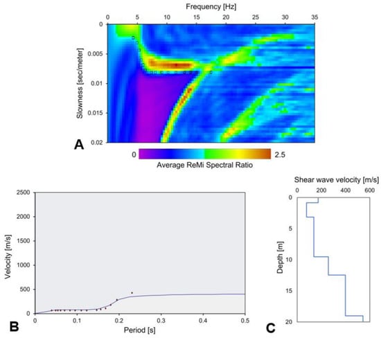
Figure 2.
(A) Sample of a generated p-f image from the ReMi surveys and the identified dispersion curve and picks (black box) in the ReMi Vspect module. (B) Fitting of dispersion curve model into the dispersion picks in the ReMi Disper module. (C) Corresponding one-dimensional shear wave velocity profile from the dispersion curve model.
Vertical variations of shear wave velocities on the upper 20 m of the sites are illustrated in Figure 3. For most of the sites, the shear wave velocity of the upper 20 m generally ranged from ~100 m/s to ~220 m/s, corresponding to SPT-N values typically ranging from 2–10. For sites with much stiffer strata, the Vs at some depths can reach up to ~250 m/s to ~500 m/s. This was in areas with higher recorded N-values, that ranged from 15 to 50. In terms of the average Vs of the upper 30 m of the sites (Vs30), most of the western portion of Metro Manila was classified into Site Class D, based on the scheme of the National Structural Code of the Philippines [48]. This indicates that the area is generally underlain by stiff soil material, with a Vs30 ranging from 180–360 m/s. This was also observed in the data obtained from the refraction microtremor surveys, as the Vs30 of the sites mostly fell in the Site D range.
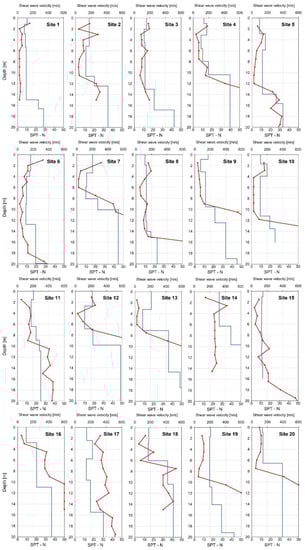
Figure 3.
Variation of shear wave velocity (Vs) and penetration resistance (SPT-N) with depth for all twenty sites. Legend: blue lines for shear wave velocities; red lines for SPT-N values.
4. Methodology
A regression analysis is a statistical technique employed for analyzing empirical relationships between a dependent variable and one or more independent variables. This technique can be primarily applied to infer a relationship between the dependent and independent variable in a fixed dataset. It can also help in the visualization of variation of the values of the dependent variable, when one of the independent variables is adjusted while keeping the other independent variables constant. A particular type of regression analysis, the non-linear regression technique involves the modelling of the observed dependent variables using a mathematical function that combines one or more independent variables in a non-linear function. Power functions, exponential functions, logarithmic functions, and trigonometric functions are several typical examples of non-linear regression functions.
In this research, a power function was employed to correlate the estimated shear wave velocities, to measure the SPT-N values. This non-linear function is widely utilized in rapid evaluation of Vs and associated geotechnical parameters. The power function has a basic form of
where x and y are two variables, with x as the independent variable and where y is the response variable, while a and b are parameters of the power function [49]. a is a constant controlling the amplitude of the function, and b controls the relationship curve. This research examined the correlation based upon corrected and uncorrected SPT-N values and the Vs, irrespective of the depth, overburden pressure, geologic age of the deposit, and fines content.
Applying the natural logarithm function to Equation (1) transforms the non-linear function into a linear regression equation with the form
where Y′ = ln y, b0 = ln a, b1 = b, and X′ = ln x. The parameters of regression b0 and b1 are determined using the least squares method
with xi substituted by ln x, yi by ln y, and n as the number of data points. When the values of b0 and b1 are determined, then the original parameters of the power function at Equation (1), a and b, can be also be calculated.
To measure the quality of the non-linear regression analysis, various statistical parameters need to be determined as well. The residual (εi) of the regression analysis is the difference from the observed value (yi) of the dependent variable in comparison to its predicted value (yi*), using the regression function (Equation (5)).
The total variability (SYY) of the dependent variable (yi) is determined from two components: the (1) variability in the observations of the yi, which is accounted for by the regression function (SSR); and the (2) residual variation, which is left unexplained by the regression function (SSE) [49]. The method of determining SYY is shown in Equations (6) and (7). In these equations, is the average of the observed values of the dependent variable.
The coefficient of regression (R2) is the fraction of the total variability in the dependent variable that is accounted for by the regression function. This has a value that ranges from 0 to 1 and is expressed as
To define the strength and nature of relationship between the dependent and independent variables, the coefficient of correlation (r) is also determined [49,50]. This value is expressed as
Another method to examine the quality of the obtained correlation is to determine Spearman’s rank correlation coefficient (rs) [50,51]. This non-parametric measure of correlation utilizes ranks to measure the correlation between an independent and response variable. The ordered datasets are replaced by rankings and the correlation coefficient (rs) is calculated on the ranks, measuring the strength of association between the two ranked variables. This coefficient indicates how closely two sets of rankings agree with each other. rs is obtained using the equation
where di is the difference between the ranks and n is the number of members for each parameter. For the purposes of this work, the smallest value of each parameter (i.e., SPT N-values, shear wave velocities) was assigned with rank 1, and the rest of the dataset were ranked subsequently, in increasing order. Identical values in a dataset were assigned a rank equal to the average of their positions in the ascending order of values.
Aside from calculating different statistical parameters, graphical analysis of residuals can also be used to evaluate the proposed correlations. Histograms of standardized residuals can identify potential outliers and can determine whether the variance is normally distributed. A probability–probability (p-p) plot compares the empirical cumulative distribution function with a theoretical cumulative distribution function. p-p plots can determine if a model follows the assumed normality, as the points must follow the 1:1 diagonal line to be normally distributed data.
5. Results and Discussion
Several empirical relations of shear wave velocity (Vs) and penetration resistance (N) have been developed by a variety of researchers. In some references, corrected N-values were used in the regression analysis. These empirical correlations are summarized in Table 2. These correlations have a basic power law form Vs = a × Nb, where a and b are coefficients that govern the shape of the empirical function. From Table 2, it is observable that for all previously proposed empirical correlations, a typically ranges from 19 to 121 and b ranges from 0.24 to 0.85.
Table 2.
Existing correlation between shear wave velocity and standard penetration resistance.
5.1. All Soils
This study utilized 265 data pairs from 20 sites in Metro Manila to propose new Vs–N empirical correlations for all soil types (Figure 4A). The empirical correlations were developed using non-linear regression analysis to fit the power law form. The proposed correlation from the data of this study is
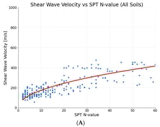
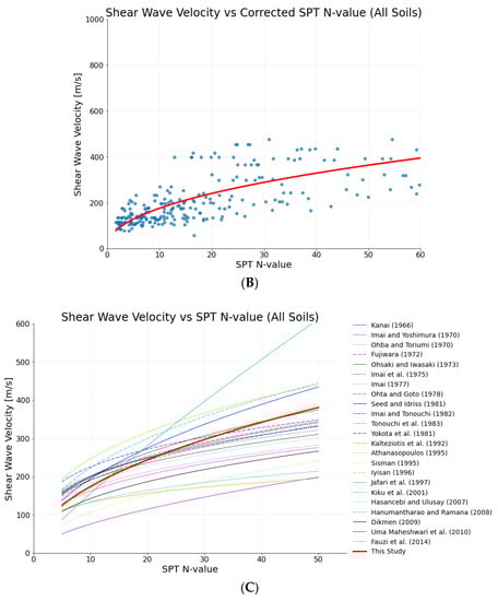
Figure 4.
(A). Uncorrected SPT-N and Vs pairs for all soils and the determined empirical correlation. (B). Corrected SPT-N and Vs pairs for all soils and the determined empirical correlation. (C). Comparison of the proposed empirical correlation for all soil types and other published works [8,9,12,13,14,15,16,21,23,26,28,30,34,35,52,53,57,61,63,64,65,67,72].
This relation has a regression coefficient R2 = 0.7515, which indicates a strong correlation between the datasets [68]. Empirical correlations for the soil types proposed by other researchers were also compiled and compared to the results of this study (Figure 4C). In this compilation, for correlations that follow the form Vs = a × Nb, the values of a range from 19 to 121 and b ranges from 0.24 to 0.85 can be observed. Among the compiled research that published empirical correlations, only Hasancebi and Ulusay (2007) [28] utilized corrected SPT-N values. On the other hand, Jinan (1987) [58] also proposed a correlation with a form Vs = a (N + b)c.
It can be observed that the correlation by Kanai (1966) [52] can be used as the lower bound, while the work of Athanasopoulos (1995) [23] and Jafari et al. (1997) [64] provide a suitable upper bound for the proposed empirical relation of this study. The other twenty-one correlations were constrained by these three functions. Furthermore, the proposed curve of the present study lies closest to that proposed by Iyisan (1996) [26].
This study also explored correlating the shear wave velocity to corrected SPT-N values by applying several correction factors (Figure 4B). These correction factors are for the rod length (CR), sampling method (CS), borehole diameter (CB), energy ratio (CE), and overburden pressure (CN). There are different equations for the correction of SPT-N values (N1)60, but the equation applied in this work is as follows:
For overburden pressure correction, we adapted the equation proposed by Kayen et al. (1992) [69], which is as follows:
σ′vo is the effective overburden pressure at the depth in kPa, and Pa is the reference pressure equal to 100 kPa. Rod length correction (CR) was applied using the factors provided by Youd et al. (2001) [70]. A sampling method (CS) correction factor of 1 was used, as most SPT drillings in the Philippines utilize standard samplers. Borehole diameter (CB) and energy ratio (CE) factors were applied following the scheme of Skempton (1986) [71]. After the application of these correction factors, non-linear regression analysis was employed again, to determine the empirical function to correlate Vs and corrected SPT-N values.
The determined correlation from the data is
This relation has a regression coefficient R2 = 0.5685, indicating a moderate correlation, which is slightly lower than the regression coefficient when uncorrected SPT-N values are used in the analysis. This suggests that uncorrected SPT-N values correlate shear wave velocity better than corrected values.
5.2. Sandy Soils
A similar non-linear regression analysis was applied for sandy soil materials. Out of the 265 data points, 139 were identified to be of sandy soil. The proposed correlation for sandy soil types is
This proposed correlation has a coefficient of regression value of R2 = 0.7922. This value is relatively higher than the coefficient for all soil types and can be regarded as a strong correlation [68]. Figure 5 shows the plotted Vs and N-value for sandy soil and the corresponding proposed empirical relation. The empirical correlations for sandy soils proposed by other researchers were also compiled. Thirteen correlations follow the power law form Vs = a × Nb while utilizing the uncorrected SPT-N values in the analysis, while Pitilakis et al. (1999) [22] and Hasancebi and Ulusay (2007) [28] utilized corrected N-values for their statistical analysis. From the compiled curves, the a coefficient ranges from 31.7 to 162, while the b coefficient ranges from 0.17 to 0.54. On the other hand, Fumal and Tinsley (1985) [56] and Kayabali (1996) [27] proposed an empirical relation with the form Vs = a(N + b)c.
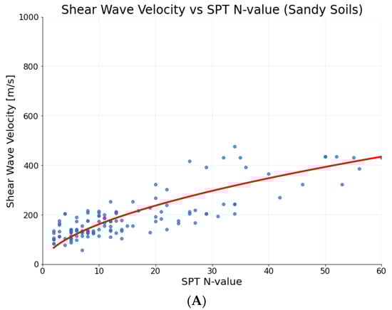
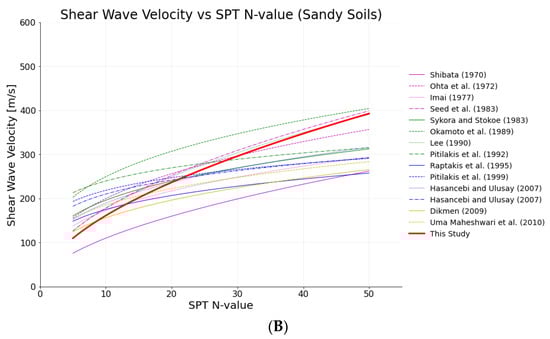
Figure 5.
(A). Uncorrected SPT-N and Vs pairs for sandy soils and the determined empirical correlation. (B). Comparison of the proposed empirical correlation for sandy soil types and other published works [10,11,14,18,22,24,28,30,35,55,59,60,62].
When the proposed empirical relation is compared to the works of other researchers, it can be observed that the relations proposed by Okamoto et al. (1989) [59] and Shibata (1970) [10] can act as the upper and lower limits for empirical relationships for sandy soil types, respectively. The other eleven published empirical relations lie between these constraints, including the one proposed by this study. As the curve of this present study lies in the middle of all the other curves, this indicates a very good agreement with respect to the previous works.
5.3. Clayey Soils
A non-linear regression analysis was also applied to clayey soil types. A total 120 data pairs of Vs-SPT-N values were identified and utilized for the statistical analysis. The proposed correlation for clayey soil in this study is
This proposed correlation has a coefficient of regression value of R2 = 0.73. This value is relatively lower than the coefficient for all soil types but can still be regarded as having a strong correlation [68]. Figure 6 illustrates the plotted data pairs of Vs and N-values for clayey soil and the corresponding empirical relations. Empirical relations proposed by other authors were also compiled and compared. Eight correlation functions used the basic power law function while incorporating uncorrected SPT-N values in the analysis. In this compilation, coefficient a ranges from 27 to 114.43, and coefficient b ranges from 0.217 to 0.73.
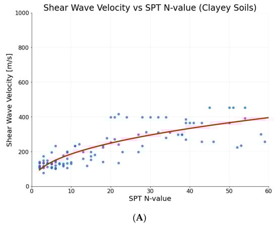
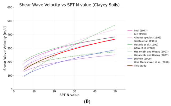
Figure 6.
(A). Uncorrected SPT-N and Vs pairs for clayey soils and the determined empirical correlation. (B). Comparison of the proposed empirical correlation for clayey soil types and other published works [14,22,23,28,30,35,60,61,66].
It can be observed from the compiled empirical curves for clayey soils that the functions by Pitilakis et al. (1999) [22] and Athanasopoulos (1995) [23] can serve as the upper bound of the proposed relations, with the curve of Pitilakis et al. (1999) [22] for N values less than 22 and N values greater than 22 for Athanasopoulos (1995) [23]. For the lower bound, the curve by Dikmen (2009) [30] can be applied for N-values less than 24. Further constraints by Imai (1977) [14] can be applied as a lower bound for N-values greater than 24. The other empirical relations lie within these boundaries, including the one proposed in this study for clayey soils. As this curve lies in the middle of the other published curves, this is an indication of the good agreement between the proposed relation and the other published works. It can also be noticed that the curve proposed by this study lies close to the work by Uma Maheshwari et al. (2010) [35].
5.4. Statistical Evaluation
Several methods were used to evaluate the proposed Vs-SPT-N values empirical relationships for all, sandy, and clayey soil types (Table 3). From the regression analysis, evaluated regression lines have an R2 that ranges from 0.73 to 0.80, suggesting a moderate to strong fit of the proposed empirical function to the obtained dataset. Evaluation using the coefficient of correlation (r) and the Spearman rank coefficient (rs) suggested that there is moderate to strong correlation between the Vs and SPT-N values from the dataset.
Table 3.
Summary of the proposed correlations from this study.
An alternative method applied to evaluate the validity of the proposed empirical relations was through an analysis of the residuals. Graphical methods for analyzing the residuals applied in this research included the development of residual histograms and probability–probability (p-p) plots (Figure 7). Histogram plots of the residuals determined whether the variance of the datasets was normally distributed. An ideal histogram of the residuals, which follows a bell-shaped distribution and which is distributed around zero, suggests that the normality assumption is likely true. In this analysis, histograms were produced from standardized residual values, which is solely the raw residual divided by its standard error. The method of standardizing residuals is applied to transform data, such that its mean centers at zero and the standard deviation equals one. This technique also identified potential outliers, such that residuals with standard deviations less than −3 or greater than 3, could be identified. In this analysis, histograms from the datasets suggested that the residuals generally followed a normal distribution, and outliers with standard deviations greater than |3| were not detected.
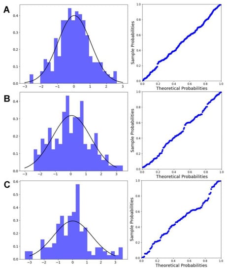
Figure 7.
Histogram of the standardized residuals and the probability–probability (p-p) plots for (A) all soils, (B) sandy soils, and (C) clayey soils.
The second graphical technique applied was a p-p plot. This type of plot compares the empirical cumulative distribution function with the theoretical cumulative distribution function. Moreover, this plot can also show whether the residuals or errors follow the assumed normality. Points on the p-p plot must follow the 1:1 diagonal line for normally distributed data.
Finally, the measured Vs and estimated Vs from each empirical correlation were compared, in order to assess the performance of the regression models (Figure 8). Data pairs mostly lay in the region between the lines 1:1.50 and 1:0.65.
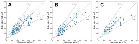
Figure 8.
Measured versus estimated Vs for (A) all soils, (B) sandy soils, and (C) clayey soils with lines of 1:1.5, 1:1 and 1:0.65.
5.5. Application for Site-Specific Characterization
One of the main applications of these empirical correlations is the estimation of the average shear wave velocity of the upper 30 m of a site (Vs30). This metric is generally used for the classification of sites into the general characteristic of the subsurface, for earthquake engineering design. In the Philippines, Vs30 is the most important parameter needed for the site classification scheme stipulated by the National Structural Code of the Philippines (2015) [44]. This scheme classifies a site into six categories used for earthquake engineering design (Table 4).
Table 4.
Site classification scheme according to the National Structural Code of the Philippines, employing the Vs30 metric to determine the general soil description and its typical corresponding N-values.
The magnitude of Vs30 can be computed in accordance with the expression
where hi and vi are the layer thickness (m) and shear wave velocity (m/s) of the ith layer, respectively, in a total of n layers existing in the top 30-m of a site. The magnitude of the Vs is estimated from SPT-N values using the proposed empirical relations applicable for all soil types. Sample boreholes with penetration depths reaching 30 m were examined, and the proposed empirical correlation was applied to the datasets (Table 5). The calculated Vs30s highlight the site classifications obtained from SPT data. Site Class D classification is dominant in Metro Manila, particularly on the western sector of the region along the coast. This suggests that the sites are generally underlain by stiff soil deposits. This is further supported by the Quaternary Alluvium deposits mapped along the western coast, proximal to Manila Bay.
Table 5.
Typical average shear wave velocity to a 30-m depth (Vs30) of all soils at various locations in Metro Manila.
An additional utility of these correlations is in the refinement of the corresponding N-values for a specific range of shear wave velocities. Based on the outcomes of this study, a simplified correlation can be established for basic soil strength classification (i.e., soft soils, stiff soils, and very dense soils) (Table 6).
Table 6.
Simplified correlation of Vs and SPT-N for different soil strength classifications in this study.
This demonstrates the utility of the proposed empirical correlations for geotechnical description at site-specific scales, as well as seismic microzonation efforts in the study area. Specific ranges of Vs have a corresponding range of N-values, where geophysical measurements of Vs can complement point borehole profiles and establish the lateral continuity of subsurface material between drilling points. In situations where SPT boreholes might not be feasible, due to economic or logistic reasons, refraction microtremor or other geophysical tests that can reliably measure shear wave velocities and can serve as a proxy to determine the relative strength of soils, especially for smaller construction projects. This was demonstrated by Pancha and Apperley (2021) [73], through utilizing refraction microtremors in two-dimensional shear wave velocity mapping, thereby extending subsurface characterization and mapping lateral variations between spot boreholes.
Alternatively, shear wave velocity surveys might not be feasible in some urban areas, due to a lack of availability of open space to lay the linear geophone array, which is a technical requirement of some geophysical tests. These sites instead might have robust borehole survey results acquired before the building’s construction. Compilation of these SPT datasets can be utilized and converted to shear wave values, to produce or refine seismic microzonation maps. The derived empirical correlations of Vs and reliable static field data such as the SPT N-value can be an alternative way to determine these seismic parameters, such as the Vs30.
However, an important caveat, before the application of the proposed empirical relations, is to ensure the reliability of obtained SPT data to estimate the corresponding Vs values. On the other hand, the processing of geophysical data to acquire Vs must also be performed with utmost caution, to minimize uncertainty before applying it for basic soil strength classification. Furthermore, these empirical correlations must be applied with caution and with consideration to the geologic, geomorphologic, and geotechnical setting of an area. Areas with a very different environment must utilize other empirical functions that are more suitable to the locality.
6. Conclusions
By utilizing 265 pairs of SPT-N values and Vs, empirical relations between the two variables were developed for the area of Metro Manila, Philippines. Data from field surveys using standard penetration tests and refraction microtremor were obtained in 20 sites in Metro Manila, all situated along the western coast of the region and underlain by unconsolidated Quaternary Alluvium deposits. These datasets were mainly grouped into three: all soils, sandy soils, and clayey soil types. New empirical relations were determined using non-linear regression analysis. To evaluate the statistical validity of the empirical models, parameters such as coefficient of regression (R2), coefficient of correlation (r), and Spearman rank correlation (rs) were determined for each soil grouping. The determined values from these coefficients (R2: 0.73–0.79, r: 0.84–0.90, rs: 0.81–0.85) suggested a moderate to strong correlation between the two parameters. Moreover, residual histograms and probability–probability plots were also produced, to graphically analyze the datasets and evaluate the proposed empirical functions. This analysis showed the presumed normality distribution of the residuals and therefore supported the validity of the empirical models. The newly developed empirical correlations for the three categories of soil are comparable to other works on this subject by researchers around the world. This suggests that the new correlations can be applied for site-specific seismic characterizations. This was demonstrated by estimating magnitudes of Vs30 from SPT-N values, which were consistent with pre-identified site classifications. This shows the utility of the proposed correlations for seismic microzonation efforts in the study area, as long as there are reliable SPT values.
Author Contributions
Conceptualization, A.S.D., O.P.C.H., A.A.T.M. and R.N.G.; methodology, A.S.D., O.P.C.H., A.A.T.M. and R.N.G.; formal analysis, O.P.C.H. and A.A.T.M.; investigation, O.P.C.H. and A.A.T.M.; writing—original draft preparation, O.P.C.H. and A.A.T.M.; writing—review and editing, A.S.D., R.N.G. and R.U.S.J. All authors have read and agreed to the published version of the manuscript.
Funding
This research was funded by the Republic of the Philippines—Department of Science and Technology (DOST) and Philippine Council for Industry, Energy and Emerging Technology (DOST-PCIEERD) Grants-in-Aid (GIA).
Institutional Review Board Statement
Not applicable.
Informed Consent Statement
Not applicable.
Data Availability Statement
Not applicable.
Acknowledgments
The authors would like to thank A.T. Serrano, M.J.V. Reyes, A.O. Amandy L.E.G. Aque, M.C.Dela Cruz, K.S. Sochayseng, E.J.M. Arnoco, and O.S. Locaba for assistance in data acquisition; M.I.T. Abigania, M.P. Dizon, D. Buhay, and E. Mitiam for rendering further technical support; the Specific Earthquake Project of DOST-PHIVOLCS for lending the Refraction Microtremor data processing software. We also thank the Department of Education for their participation in this research.
Conflicts of Interest
The authors declare no conflict of interest.
References
- Duan, W.; Cai, G.; Liu, S.; Puppala, A.J. Correlations between Shear Wave Velocity and Geotechnical Parameters for Jiangsu Clays of China. Pure Appl. Geophys. 2019, 176, 669–684. [Google Scholar] [CrossRef]
- Gautam, D. Empirical Correlation between Uncorrected Standard Penetration Resistance (N) and Shear Wave Velocity (VS) for Kathmandu Valley, Nepal. Geomat. Nat. Hazards Risk 2017, 8, 496–508. [Google Scholar] [CrossRef]
- Andrus, R.D.; Stokoe, K.H.; Hsein Juang, C. Guide for Shear-Wave-Based Liquefaction Potential Evaluation. Earthq. Spectra 2004, 20, 285–308. [Google Scholar] [CrossRef]
- Kayen, R.; Moss, R.E.S.; Thompson, E.M.; Seed, R.B.; Cetin, K.O.; Kiureghian, A.D.; Tanaka, Y.; Tokimatsu, K. Shear-Wave Velocity–Based Probabilistic and Deterministic Assessment of Seismic Soil Liquefaction Potential. J. Geotech. Geoenviron. Eng. 2013, 139, 407–419. [Google Scholar] [CrossRef]
- Mohamed, A.M.E.; Abu El Ata, A.S.A.; Abdel Azim, F.; Taha, M.A. Site-Specific Shear Wave Velocity Investigation for Geotechnical Engineering Applications Using Seismic Refraction and 2D Multi-Channel Analysis of Surface Waves. NRIAG J. Astron. Geophys. 2013, 2, 88–101. [Google Scholar] [CrossRef][Green Version]
- Sasitharan, S.; Robertson, P.K.; Sego, D.C. Sample Disturbance from Shear Wave Velocity Measurements. Can. Geotech. J. 1994, 31, 119–124. [Google Scholar] [CrossRef]
- Ghazi, A.; Moghadas, N.H.; Sadeghi, H.; Ghafoori, M.; Lashkaripur, G.R. Empirical Relationships of Shear Wave Velocity, SPT-N Value and Vertical Effective Stress for Different Soils in Mashhad, Iran. Ann. Geophys. 2015, 58, 2. [Google Scholar] [CrossRef]
- Imai, T.; Yoshimura, Y. Elastic Wave Velocity and Soil Properties in Soft Soil. Tsuchi-ToKiso 1970, 18, 17–22. (In Japanese) [Google Scholar]
- Ohba, S.; Toriumi, I. Dynamic Response Characteristics of Osaka Plain. In Proceedings of the Annual Meeting, Architectural Institure of Japan, Tokyo, Japan, 5 October 1970. [Google Scholar]
- Shibata, T. The Relationship between the N-Value and S-Wave Velocity in the Soil Layer; Disaster Prevention Research Laboratory, Kyoto University: Kyoto, Japan, 1970. [Google Scholar]
- Ohta, T.; Hara, A.; Niwa, M.; Sakano, T. Elastic Shear Moduli as Estimated from N-Value. In Proceedings of the 7th Annual Convention of Japan Society of Soil Mechanics and Foundation Engineering, Tokyo, Japan, 10–15 July 1972; pp. 265–268. [Google Scholar]
- Fujiwara, T. Estimation of Ground Movements in Actual Destructive Earthquakes. In Proceedings of the Fourth European Symposium on Earthquake Engineering, London, UK, 5–7 September 1972; pp. 125–132. [Google Scholar]
- Ohsaki, Y.; Iwasaki, R. On Dynamic Shear Moduli and Poisson’s Ratios of Soil Deposits. Soils Found. 1973, 13, 61–73. [Google Scholar] [CrossRef]
- Imai, T. P and S Wave Velocities of the Ground in Japan. In Proceedings of the IX International Conference on Soil Mechanics and Foundation Engineering, Tokyo, Japan, 10–15 July 1977; pp. 127–132. [Google Scholar]
- Imai, T.; Tonouchi, K. Correlation of N-Value with S-Wave Velocity and Shear Modulus. In Proceedings of the 2nd European Symposium of Penetration Testing, Amsterdam, The Netherlands, 24–27 May 1982; pp. 57–72. [Google Scholar]
- Seed, H.B.; Idriss, I.M. Evaluation of Liquefaction Potential Sand Deposits Based on Observation of Performance in Previous Earthquakes. In Proceedings of the ASCE National Convention 1981, St. Louis, MO, USA, 26–30 October 1981; pp. 481–544. [Google Scholar]
- Seed, H.; Tokimatsu, K.; Harder, L.F.; Chung, R.M. Influence of SPT Procedures in Soil Liquefaction Resistance Evaluations. J. Geotech. Eng. 1985, 111, 1425–1445. [Google Scholar] [CrossRef]
- Sykora, D.E.; Stokoe, K.H. Correlations of In-Situ Measurements in Sands of Shear Wave Velocity. Soil Dyn. Earthq. Eng. 1983, 20, 125–136. [Google Scholar]
- Rollins, K.M.; Evans, M.D.; Diehl, N.B.; Iii, W.D.D. Shear Modulus and Damping Relationships for Gravels. J. Geotech. Geoenviron. Eng. 1998, 124, 396–405. [Google Scholar] [CrossRef]
- Brandenberg, S.J.; Bellana, N.; Shantz, T. Shear Wave Velocity as Function of Standard Penetration Test Resistance and Vertical Effective Stress at California Bridge Sites. Soil Dyn. Earthq. Eng. 2010, 30, 1026–1035. [Google Scholar] [CrossRef]
- Kalteziotis, N.; Sabatakakis, N.; Vassiliou, J. Evaluation of Dynamic Characteristicsof Greek Soil Formations. In Proceedings of the 2nd Hellenic Conference on Geotechnical Engineering, Thessaloniki, Greece, 28 September–1 October 1992; pp. 239–246. [Google Scholar]
- Pitilakis, K.; Raptakis, D.; Lontzetidis, K.; Tika-Vassilikou, T.; Jongmans, D. Geotechnical and Geophysical Description of Euro-Seistest Using Field, Laboratory Tests and Moderate Strong Motion Recordings. J. Earthq. Eng. 1999, 3, 381–409. [Google Scholar] [CrossRef]
- Athanasopoulos, G. Empirical Correlations Vs-N SPT for Soils of Greece: A Comparative Study of Reliability. In Proceedings of the 7th International Conference on Soil Dynamics and Earthquake Engineering, Crete, Greece, 7 May 1995; pp. 19–36. [Google Scholar]
- Raptakis, D.G.; Anastasiadis, S.A.J.; Pitilakis, K.D.; Lontzetidis, K.S. Shear Wave Velocities and Damping of Greek Natural Soils. In Proceedings of the 10th European Conference on Earthquake Engineering, Vienna, Austria, 28 August–2 September 1994; pp. 477–482. [Google Scholar]
- Tsiambaos, G.; Sabatakakis, N. Empirical Estimation of Shear Wave Velocity from in Situ Tests on Soil Formations in Greece. Bull. Eng. Geol. Environ. 2011, 70, 291–297. [Google Scholar] [CrossRef]
- Iyisan, R. Correlations between Shear Wave Velocity and In-Situ Penetration Test Results. Chamb. Civ. Eng. Turk. Tek. Dergi 1996, 7, 1187–1199. [Google Scholar]
- Kayabali, K. Soil Liquefaction Evaluation Using Shear Wave Velocity. Eng. Geol. 1996, 44, 121–127. [Google Scholar] [CrossRef]
- Hasancebi, N.; Ulusay, R. Empirical Correlations between Shear Wave Velocity and Penetration Resistance for Ground Shaking Assessments. Bull. Eng. Geol. Environ. 2007, 66, 203–213. [Google Scholar] [CrossRef]
- Koçkar, M.K.; Akgün, H. Development of a Geotechnical and Geophysical Database for Seismic Zonation of the Ankara Basin, Turkey. Env. Geol. 2008, 55, 165–176. [Google Scholar] [CrossRef]
- Dikmen, Ü. Statistical Correlations of Shear Wave Velocity and Penetration Resistance for Soils. J. Geophys. Eng. 2009, 6, 61–72. [Google Scholar] [CrossRef]
- Akin, M.K.; Kramer, S.L.; Topal, T. Empirical Correlations of Shear Wave Velocity (Vs) and Penetration Resistance (SPT-N) for Different Soils in an Earthquake-Prone Area (Erbaa-Turkey). Eng. Geol. 2011, 119, 1–17. [Google Scholar] [CrossRef]
- Anbazhagan, P.; Sitharam, T.G. Relationship between Low Strain Shear Modulus and Standard Penetration Test N Values. Geotech. Test. J. 2010, 33, 102278. [Google Scholar] [CrossRef]
- Anbazhagan, P.; Kumar, A.; Sitharam, T.G. Seismic Site Classification and Correlation between Standard Penetration Test N Value and Shear Wave Velocity for Lucknow City in Indo-Gangetic Basin. Pure Appl. Geophys. 2013, 170, 299–318. [Google Scholar] [CrossRef]
- Hanumantharao, C.; Ramana, G.V. Dynamic Soil Properties for Microzonation of Delhi, India. J. Earth Syst. Sci. 2008, 117, 719–730. [Google Scholar] [CrossRef]
- Uma Maheswari, R.; Boominathan, A.; Dodagoudar, G.R. Use of Surface Waves in Statistical Correlations of Shear Wave Velocity and Penetration Resistance of Chennai Soils. Geotech. Geol. Eng. 2010, 28, 119–137. [Google Scholar] [CrossRef]
- Kuo, C.-H.; Wen, K.-L.; Hsieh, H.-H.; Chang, T.-M.; Lin, C.-M.; Chen, C.-T. Evaluating Empirical Regression Equations for Vs and Estimating Vs30 in Northeastern Taiwan. Soil Dyn. Earthq. Eng. 2011, 31, 431–439. [Google Scholar] [CrossRef]
- Gervacio, F. The Geology, Structures, and Landscape Development of Manila and Suburbs. Philipp. Geol. 1968, 21, 178–192. [Google Scholar]
- Bureau of Mines and Geosciences. Geological Map of Manila and Quezon City Quadrangle—Sheet 3263-IV [Map]; Bureau of Mines and Geosciences: Quezon City, Philippines, 1983.
- Japan International Cooperation Agency; Metropolitan Manila Development Agency; Philippine Institute of Volcanology and Seismology. Earthquake Impact Reduction Study for Metro Manila, Republic of the Philippines; Japan International Cooperation Agency: Makati City, Philippines, 2004.
- Miura, H.; Midorikawa, S.; Fujimoto, K.; Pacheco, B.M.; Yamanaka, H. Earthquake Damage Estimation in Metro Manila, Philippines Based on Seismic Performance of Buildings Evaluated by Local Experts’ Judgments. Soil Dyn. Earthq. Eng. 2008, 28, 764–777. [Google Scholar] [CrossRef]
- Teves, J.S.; Gonzales, M.L. The Geology of the University Site, Balara Area, Quezon City. Phil. Geol. 1950, 4, 1–10. [Google Scholar]
- Rimando, R.E.; Knuepfer, P.L.K. Neotectonics of the Marikina Valley Fault System (MVFS) and Tectonic Framework of Structures in Northern and Central Luzon, Philippines. Tectonophysics 2006, 415, 17–38. [Google Scholar] [CrossRef]
- Tan, R.C. Engineering Properties of Manila Subsoils; University of the Philippines: Quezon City, Philippines, 1983. [Google Scholar]
- Association of Structural Engineers of the Philippines, Inc. National Structural Code of the Philippines, 7th ed.; Association of Structural Engineers of the Philippines, Inc.: Quezon City, Philippines, 2015; Volume 1. [Google Scholar]
- ASTM D1586/D1586M-18e1; Test Method for Standard Penetration Test (SPT) and Split-Barrel Sampling of Soils. ASTM International: West Conshohocken, PA, USA, 2022.
- ASTM D2487-17e1; Practice for Classification of Soils for Engineering Purposes (Unified Soil Classification System). ASTM International: West Conshohocken, PA, USA, 2022.
- Louie, J.N. Faster, Better: Shear-Wave Velocity to 100 Meters Depth from Refraction Microtremor Arrays. Bull. Seismol. Soc. Am. 2001, 91, 347–364. [Google Scholar] [CrossRef]
- Philippine Institute of Volcanology and Seismology. The Philippine Earthquake Model; Philippine Institute of Volcanology and Seismology: Quezon City, Philippines, 2017.
- Chatterjee, K.; Choudhury, D. Variations in Shear Wave Velocity and Soil Site Class in Kolkata City Using Regression and Sensitivity Analysis. Nat. Hazards 2013, 69, 2057–2082. [Google Scholar] [CrossRef]
- Rezaei, S.; Shooshpasha, I.; Rezaei, H. Empirical Correlation between Geotechnical and Geophysical Parameters in a Landslide Zone (Case Study: Nargeschal Landslide). Earth Sci. Res. J. 2018, 22, 195–204. [Google Scholar] [CrossRef]
- Lin, J.; Cai, G.; Liu, S.; Puppala, A.J.; Zou, H. Correlations Between Electrical Resistivity and Geotechnical Parameters for Jiangsu Marine Clay Using Spearman’s Coefficient Test. Int. J. Civ. Eng. 2017, 15, 419–429. [Google Scholar] [CrossRef]
- Kanai, K. Conference on Cone Penetrometer; The Ministry of Public Works and Settlement: Ankara, Turkey, 1966.
- Imai, T.; Fumoto, H.; Yokota, K. The Relation of Mechanical Properties of Soil to Pand S-Wave Velocities in Japan. In Proceedings of the 4th Japan Earthquake Engineering Symposium, Tokyo, Japan, 6 September 1975. [Google Scholar]
- Ohta, Y.; Goto, N.; Kagami, H.; Shiono, K. Shear Wave Velocity Measurement during a Standard Penetration Test. Earthq. Eng. Struct. Dyn. 1978, 6, 43–50. [Google Scholar] [CrossRef]
- Seed, H.B.; Idriss, I.M.; Arango, I. Evaluation of Liquefaction Potential Using Field Performance Data. J. Geotech. Eng. 1983, 109, 458–482. [Google Scholar] [CrossRef]
- Fumal, T.E.; Tinsley, J.C. Predicting Area Limits of Earthquake Induced Land Sliding Based on Seismological Parameters. In Evaluation of Earthquake Hazards in the Los Angeles Region–An Earth Science Prospective; U.S. Geological Survey: Los Angeles, CA, USA, 1985; pp. 127–150. [Google Scholar]
- Tonouchi, K.; Sakayama, T.; Imai, T. S Wave Velocity in the Ground and the Damping Factor. Bull. Int. Assoc. Eng. Geol. 1983, 26–27, 327–333. [Google Scholar]
- Jinan, Z. Correlation between Seismic Wave Velocity and the Number of Blow of SPT and Depth. Sel. Pap. Chin. J. Geotech. Eng. 1987, 1, 92–100. [Google Scholar]
- Okamoto, T.; Kokusho, T.; Yoshida, Y.; Kusuonoki, K. Comparison of Surface versus Subsurface Wave Source for P–Slogging in Sand Layer. In Proceedings of the 44th Annal Conference JSCE, October 1989; Volume 3, pp. 996–997. [Google Scholar]
- Lee, S.H. Regression Models of Shear Wave Velocities in Taipei Basin. J. Chin. Inst. Eng. 1990, 13, 519–532. [Google Scholar] [CrossRef]
- Yokota, K.; Imai, T.; Konno, M. Dynamic Deformation Characteristics of Soils Determined by Laboratory Tests. OYO Technical Report. 1981, p. 26. Available online: https://www.oyo.co.jp/oyocms_hq/wp-content/uploads/2014/12/1981_03.pdf (accessed on 20 June 2022).
- Pitilakis, K.D.; Anastasiadis, A.; Raptakis, D. Field and Laboratory Determination of Dynamic Properties of Natural Soil Deposits. In Proceedings of the 10th World Conference Earthquake Engineering, Rotherdam, The Netherlands, 19 July 1992; pp. 1275–1280. [Google Scholar]
- Sisman, H. An Investigation on Relationships between Shear Wave Velocity, and SPT and Pressuremeter Test Results. Master’s Thesis, Ankara University, Geophysical Engineering Department, Ankara, Turkey, 1995. [Google Scholar]
- Jafari, M.K.; Asghari, A.; Rahmani, I. Empirical Correlation between Shear Wave Velocity (Vs) and SPT-N Value for South Tehran Soils. In Proceedings of the 4th International Conference on Civil Engineering, Tehran, Iran, 4–6 May 1997. [Google Scholar]
- Kiku, H.; Yoshida, N.; Yasuda, S.; Irisawa, T.; Nakazawa, H.; Shimizu, Y.; Ansal, A.; Erkan, A. In-Situ Penetration Tests and Soil Profiling in Adapazari, Turkey. In Proceedings of the ICSMGE/TC4 Satellite Conference on Lessons Learned From Recent Strong Earthquakes, Istanbul, Turkey, 25 August 2001; pp. 259–265. [Google Scholar]
- Jafari, M.K.; Shafiee, A.; Razmkhah, A. Dynamic Properties of Fine Grained Soils in South of Tehran. J. Seismol. Earthq. Eng. 2002, 4, 25–35. [Google Scholar]
- Fauzi, A. Empirical Correlation of Shear Wave Velocity and N-SPT Value for Jakarta. Geomate 2014, 7, 980–984. [Google Scholar] [CrossRef]
- Moore, D.S.; Notz, W.; Fligner, M.A. The Basic Practice of Statistics, 6th ed.; W.H. Freeman: New York, NY, USA, 2013; ISBN 978-1-4641-0254-7. [Google Scholar]
- Kayen, R.E.; Mitchell, J.K.; Seed, R.B.; Lodge, A.; Nishio, S.; Coutinho, R. Evaluation of SPT-, CPT-, and Shear Wave-Based Methods for Liquefaction Potential Assessment Using Loma Prieta Data. In Proceedings of the 4th Japan-U.S. Workshop on Earthquake Resistant Design of Lifeline Facilities and Countermeasures for Soil Liquefaction, Honolulu, Hawaii, 27–29 May 1992; Volume 1, pp. 117–204. [Google Scholar]
- Youd, T.L.; Idriss, I.M.; Andrus, R.D.; Arango, I.; Castro, G.; Christian, J.T.; Dobry, R.; Finn, W.D.L.; Harder, L.F.; Hynes, M.E.; et al. Liquefaction Resistance of Soils: Summary Report from the 1996 NCEER and 1998 NCEER/NSF Workshops on Evaluation of Liquefaction Resistance of Soils. J. Geotech. Geoenviron. Eng. 2001, 127, 817–833. [Google Scholar] [CrossRef]
- Skempton, A.W. Standard Penetration Test Procedures and the Effects in Sands of Overburden Pressure, Relative Density, Particle Size, Ageing and Overconsolidation. Géotechnique 1986, 36, 425–447. [Google Scholar] [CrossRef]
- Ohta, Y.; Goto, N. Empirical Shear Wave Velocity Equations in Terms of Characteristic Soil Indexes. Earthquake Engng. Struct. Dyn. 1978, 6, 167–187. [Google Scholar] [CrossRef]
- Pancha, A.; Apperley, R.A. Multidisciplinary Site Investigations: Refraction Microtremor Surveys. J. Seism. 2021, 1–14. [Google Scholar] [CrossRef]
Publisher’s Note: MDPI stays neutral with regard to jurisdictional claims in published maps and institutional affiliations. |
© 2022 by the authors. Licensee MDPI, Basel, Switzerland. This article is an open access article distributed under the terms and conditions of the Creative Commons Attribution (CC BY) license (https://creativecommons.org/licenses/by/4.0/).