Article

Typhoon Track Prediction Based on Deep Learning

1
The Institute of Naval Industrial Design, Shandong University of Art & Design, Qingdao 266555, China
2
The Institute of Data Science, City University of Macau, Taipa 999078, Macau
3
The Laboratory of Marine Intelligent Equipment, Hainan University, Haikou 570100, China
*
Author to whom correspondence should be addressed.
Appl. Sci. 2022, 12(16), 8028; https://doi.org/10.3390/app12168028
Submission received: 21 July 2022 / Revised: 5 August 2022 / Accepted: 8 August 2022 / Published: 11 August 2022
(This article belongs to the Special Issue Multi-Modal Deep Learning and Its Applications)

Abstract

:
China is located in the northwest Pacific region where typhoons occur frequently, and every year typhoons make landfall and cause large or small economic losses or even casualties. Therefore, how to predict typhoon paths more accurately has undoubtedly become an important research topic nowadays. Therefore, this paper predicts the path of typhoons formed in the South China Sea based on deep learning. This paper combines the CNN network and the LSTM network to build a C-LSTM typhoon path prediction model, using the typhoon paths and related meteorological variables formed in the South China Sea from 1949 to 2021 as the data set, and using the Granger causality test to select multiple features for the data set to achieve data dimensionality reduction. Finally, by comparing the experiments with the LSTM typhoon path prediction model, it is proved that the prediction results of the model have smaller errors.

1. Introduction

A typhoon is a natural phenomenon with functions, such as maintaining heat balance and regulating the heat distribution of the earth, but it is also a catastrophic weather system with super destructive power [1], which causes large or small economic losses or even human casualties to the global typhoon origin sea and its coastal areas every year [2]. With a long coastline and in the typhoon-prone northwest Pacific region, China is one of the countries in the world most affected by typhoons. Hainan, located in the South China Sea, is one of the sources of typhoons in the northwest Pacific Ocean, and the influence of the tropical monsoon, known as the “typhoon corridor”, every year in the summer and autumn, typhoons in the coastal areas will be landed, and transport to and from the island to bring some impact and even cause economic losses and casualties. In addition, in recent years, due to global climate change, typhoons triggered by heavy rains, storm surges, and other natural disasters have shown an increasing trend in frequency and intensity, which means that typhoons in the coastal areas of Hainan people’s lives and property security threat are greater. As can be seen from Figure 1, during the period 2014–2019, typhoons ranked among the top three in frequency among all natural disasters in Hainan and were the natural disasters that caused the highest direct economic losses. According to statistics, the super typhoon “Rammasun” that landed in Hainan in 2014 caused direct economic losses of 119.5226 billion RMB and affected 3.25829 million people, which is a typhoon that caused the largest direct economic losses in Hainan Province since its founding of China [3].
Strengthening and accelerating the development of typhoon prediction technology is one of the effective means that can reduce the impact brought by typhoons. By predicting the path of typhoons and obtaining their ripple places in advance, disaster prevention departments can provide more accurate information support so that they can have a longer period to develop targeted preventive measures, thus, reducing the casualties caused by typhoons and property losses to the country and the people. That is, it is of great practical significance to strengthen and accelerate the development of typhoon prediction technology.
It is well known that countries have not stopped exploring typhoons. At present, the prediction of typhoon paths can be divided into three categories: Traditional prediction methods, machine learning-based typhoon path prediction methods, and deep learning-based typhoon path prediction methods.
Traditional forecasting methods can be divided into two categories, one is the empirical method, which combines information obtained from real-time weather maps with historical similar weather conditions with human subjective experience to forecast the typhoon path. The other is the objective method, which is based on statistics, hydrodynamics and other science to forecast typhoons, and can be subdivided into three types of methods: Dynamics-based typhoon path forecasting, statistics-based typhoon path forecasting and statistical dynamics-based typhoon path forecasting.
Dynamics-based typhoon path prediction methods can also be called numerical prediction methods, which are based on a large amount of historical data to construct the atmospheric dynamics equations and transform the typhoon prediction problem into a mathematical problem [4,5,6]. However, the equations constructed by such methods are complex and computationally intensive to solve, which will consume a lot of human and material resources, costly, and take a long time. At the same time, such methods contain some empirical and hypothetical relationships, so the possibility of errors in the prediction results is very high. Statistical-based typhoon track prediction methods are based on mathematical statistics, and they are based on a statistical analysis of a large amount of historical data to find the patterns of weather changes and the relationship between typhoon tracks and forecast factors to obtain linear regression equations and forecast typhoon tracks [7,8,9,10,11,12]. However, this type of prediction method relies heavily on historical data, and although the accuracy of the prediction results is reasonable for typhoons with similar paths and the trajectories of other typhoons with similar paths in the past, the prediction results will be more inaccurate for typhoons with more special paths (e.g., circular motion, the existence of inflection points) or when the weather is subject to drastic changes. Statistical dynamics-based typhoon path prediction methods combine the above two methods, and although these methods combine dynamics and statistics to improve the prediction accuracy, they still require large computing power and are costly.
At the end of the 20th century, with the rapid development of machine learning, a large number of machine learning algorithms emerged, so many researchers began to try machine learning-based methods for typhoon path prediction. For example, using the K-means algorithm [13], combining the principal component analysis method with stepwise regression [14], constructing a numerical forecasting system based on GRAPS [15], constructing a prediction model based on gradient boosting decision tree [16], etc. Although the accuracy has been improved, there are problems such as difficulty in feature selection, poor portability of classifiers, inability to fully automate, and poor sensitivity to changes in typhoon acceleration and deceleration.
In recent years, with the proposal and development of deep learning, many scholars have started to try to predict typhoon trajectories based on deep learning, considering its properties such as nonlinearity, strong feature extraction ability, and its ability to learn temporal and spatial features from datasets and to achieve prediction of data in complex structures. The literature [17] used Artificial Neural Network (ANN) to train typhoon satellite images and demonstrated that deep learning can be used to make predictions of typhoons. The literature [18] combined the CLIPER model and the BP neural network to predict the typhoon path, and its accuracy was improved compared with the CLIPER model. Gao et al. [19] built a typhoon path prediction model based on LSTM (Long Short-Term Memory) and found that its error size is affected by the amount of data set and is more suitable for making short-term predictions of typhoon paths. Tienfuan Kerh et al. [20] proposed a method that combines static and dynamic neural network models and treats the variables affecting the typhoon path as a time series and uses a nonlinear autoregressive network with a moving average method to predict the typhoon track, which provides a new idea and method for typhoon path prediction. In the literature [21], a classification and prediction method based on a gated unit recurrent neural network was proposed, and he first classified the typhoon using a dynamic regularization algorithm, and then the typhoon path was predicted using GRU. The prediction results of this method are not bad, but the number of typhoons classified, and the basis of classification are somewhat unknown. The literature [22] proposed a fused deep learning method for typhoon path prediction based on reanalysis information, which fuses past track data and reanalysis atmospheric images to build a neural network model with lower time cost and better real-time performance compared to other existing dynamical prediction models. Sun et al. [23] proposed a deep learning model in a distributed system, based on complex features and learned by task, for implementing a typhoon path prediction model. Mario et al. [24] used Generative Adversarial Networks (GAN) for typhoon path prediction using satellite cloud images as input, which provides a visual complement to the typhoon path prediction method, but the prediction model constructed by this method converges slowly. However, the convergence speed of the prediction model constructed by this method is slow, and the prediction effect for typhoons with inconspicuous wind eyes is poor.
In summary, it is feasible to predict typhoon paths based on deep learning, and it has the advantages of being adaptable and overcoming the interference of data from typhoons with more specific paths on model parameters. Therefore, this paper chooses to build a model based on deep learning to predict typhoon paths. In addition, the timely and accurate prediction of typhoon path has a certain guiding role for the prevention and control of natural disasters in Hainan. At the same time, the study of Hainan as the object of improving typhoon prediction capability, strengthening disaster prevention and mitigation construction, can accumulate some practical experience for the national disaster prevention and mitigation construction, and improve the national corresponding construction capacity. Therefore, the research on this topic has important practical significance.
To achieve the goal of predicting the path of typhoons generated in the South China Sea based on deep learning, this paper focuses on three main aspects.
  • Data Pre-processing
Because of the long period of the dataset and complex data sources, there are inevitably problems such as uneven data quality, so the original dataset was first screened and merged to construct the best path data set of typhoons in the South China Sea. In addition, some of the typhoon path data in the dataset, such as wind speed, central pressure, radius, and other important data, are missing, so it is necessary to fill in such missing meteorological data to lay the foundation for the subsequent improvement of prediction accuracy.
  • Multi-feature selection
Typhoon paths are affected by some variables, such as the atmospheric environment, and the performance of the prediction model is highly dependent on the data set input to it. Therefore, in this paper, before inputting the data set into the prediction model, Granger Causality Test will be performed on the data set to select the variables with greater influence on typhoon paths, remove irrelevant noise, and realize data dimensionality reduction.
  • Construction of prediction model
After the selection of multiple features, this paper will combine the CNN network, which has a stronger ability to extract special features, and the LSTM network, which has a stronger ability to deal with long time series, to build a formation C-LSTM prediction model to predict the path of typhoons forming with the South China Sea. At the same time, the experimental results are compared with the prediction results of the LSTM network model for experimental analysis.

2. Materials and Methodology

This part mainly covers data acquisition, missing data filling, multi-feature selection, and construction of a C-LSTM-based typhoon path prediction model.

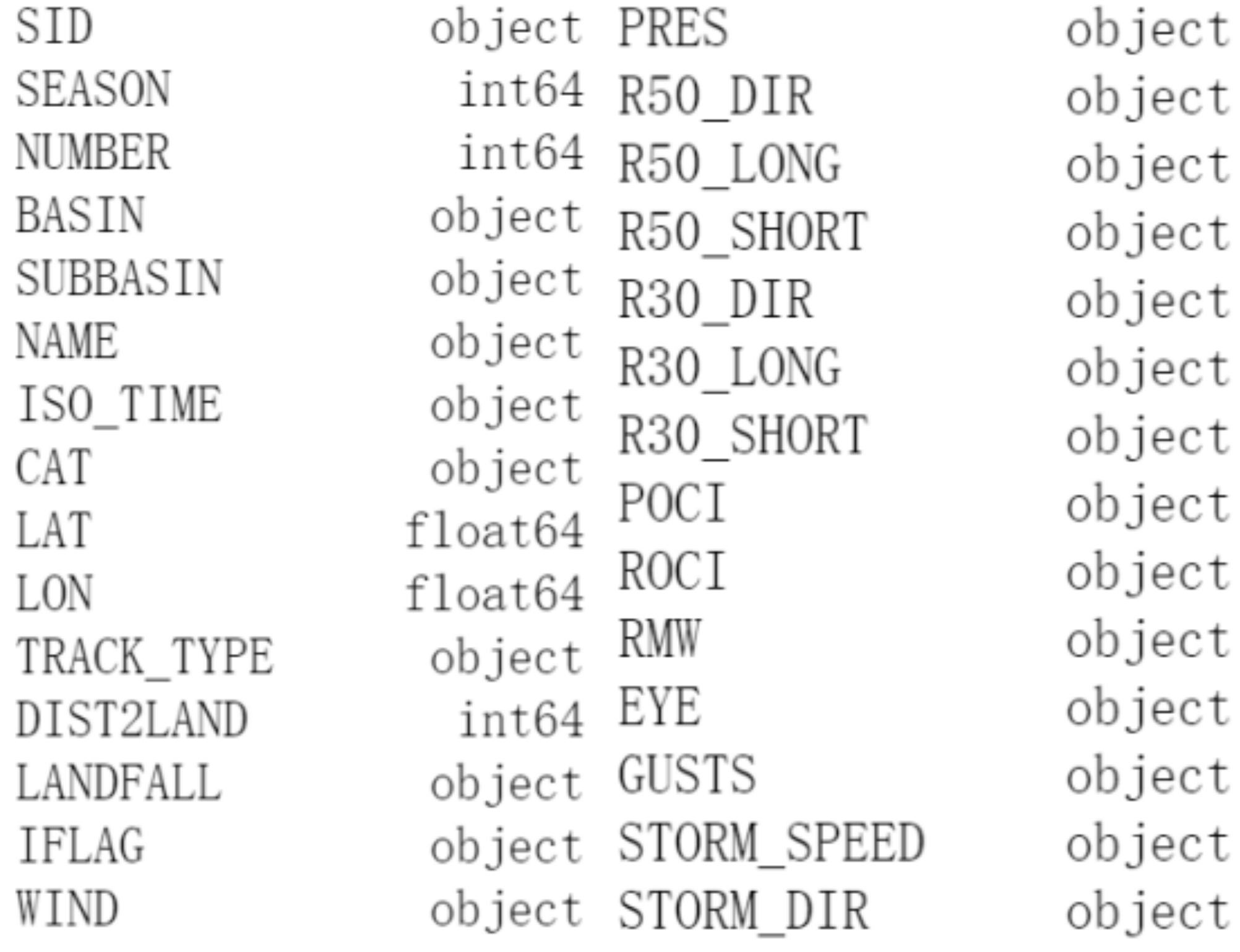
2.1. Typhoon Dataset

2.1.1. Dataset Acquisition

Because of the different levels of development in each country and the different requirements for the collection of typhoon-related data, the typhoon-related observation data recorded in each country vary in type and quality. Therefore, the best track data set of typhoons in the northwest Pacific Ocean from the official website of the National Oceanic and Atmospheric Administration (NOAA) is selected to collect the information from observatories in several countries around the world. This dataset contains 239,594 data on the paths of all typhoons formed in the northwest Pacific Ocean from 1949 to 2021 and meteorological variables affecting the paths of typhoons.
Because the research object is Hainan, only typhoons generated by the South China Sea region and requiring a relatively short landfall time are studied, so first, we need to filter their data and construct a new dataset from the data of typhoons formed by the South China Sea region among them.
At the same time, because the data sources in this dataset are complex and many of the data types in it represent the same meaning, we need to merge data from these data variables that come from multiple institutions but have repeated meanings. For the convenience of presentation, we call the dataset obtained after data filtering and merging the best path dataset of typhoons in the South China Sea. The specific composition of this dataset is shown in Table 1.
From Figure 2, we can find the data types in the dataset are not the same, so it is necessary to digitize the character type data except for the tropical cyclone number and typhoon name, i.e., to convert the data types to a numeric type. The purpose of converting the data types is to facilitate the Granger causality test and to ensure that all data in the dataset can be input as a feature that can be learned by the neural network model.
At this point, the dataset to be used in this study, the best path dataset of typhoons in the South China Sea, has been constructed. The dataset includes the path information and multiple variables of all typhoons generated by the South China Sea region from 1949 to 2021.

2.1.2. Missing Filling

Due to the long chronological span of the typhoon best track data set in the South China Sea, the data were mostly kept by manual handwriting due to the limited technical level in the early days, which easily caused data missing due to improper data storage. Before the 1970s, the satellite technology was not widely used, and the types of data recorded by various national observatories inevitably fluctuated, resulting in some missing data. The missing data will adversely affect the results of the subsequent model, so we need to deal with the missing data.
The direct deletion method is the most common and easy-to-implement method for handling missing values, but considering that multiple predictors have more or less some missing values, the direct deletion method is not used for missing processing. In addition, because these missing data also need to consider the correlation between the before and after data, they cannot be filled using the mean, plural, etc. At the same time, because the ordinary fitting method fits a function that only. In contrast, the regression equation constructed by the interpolation method will ensure that the values of all known data samples are passed, which is more stable and has guaranteed convergence. Therefore, in this paper, we choose to fill in the missing data using cubic spline interpolation.
First, the variables containing missing values in the data set were screened, and four categories of predictors, WIND, PRES, ROCI, and EYE, were found to have missing values. Subsequently, the typhoons with missing values were eliminated category by category, and four different sets of samples without missing values were obtained and normalized separately, and detailed formulas of normalization are shown in Equations (1)–(3).
μ d = i = 1 n x i n
σ d 2 = i = 1 n x i μ d n
x ^ i = x i μ d σ d 2
where μ denotes the mean of the predictors, σ 2 denotes the variance of the predictors, x ^ i denotes the normalized data values of the predictors, x i denotes the data values of the predictors, and n denotes the sample set size.
Then the missing rate was set for the sample set, the predicted values were obtained using three times spline interpolation, and the effect of data filling was evaluated by calculating the root mean square error between the predicted and observed values and the error results are shown in Table 2. The formula for calculating the root-mean-square error is shown in Equation (4).
R M S E = 1 n i = 1 n r i e i 2 i = 1 , 2 , , n
where n indicates the total number of missing values, and r i and e i indicate the true and filled values of the i th missing value, respectively. a smaller value of R M S E represents a smaller average error between the filled and true values and higher filling accuracy [25].
By observing Table 2, we can find that the R M S E of all four variables reached the level of 0.01, which is fair. Finally, the four predictors in the original dataset were filled with missingness one by one using three times spline interpolation.

2.2. Typhoon Path Prediction Model Based on C-LSTM Network

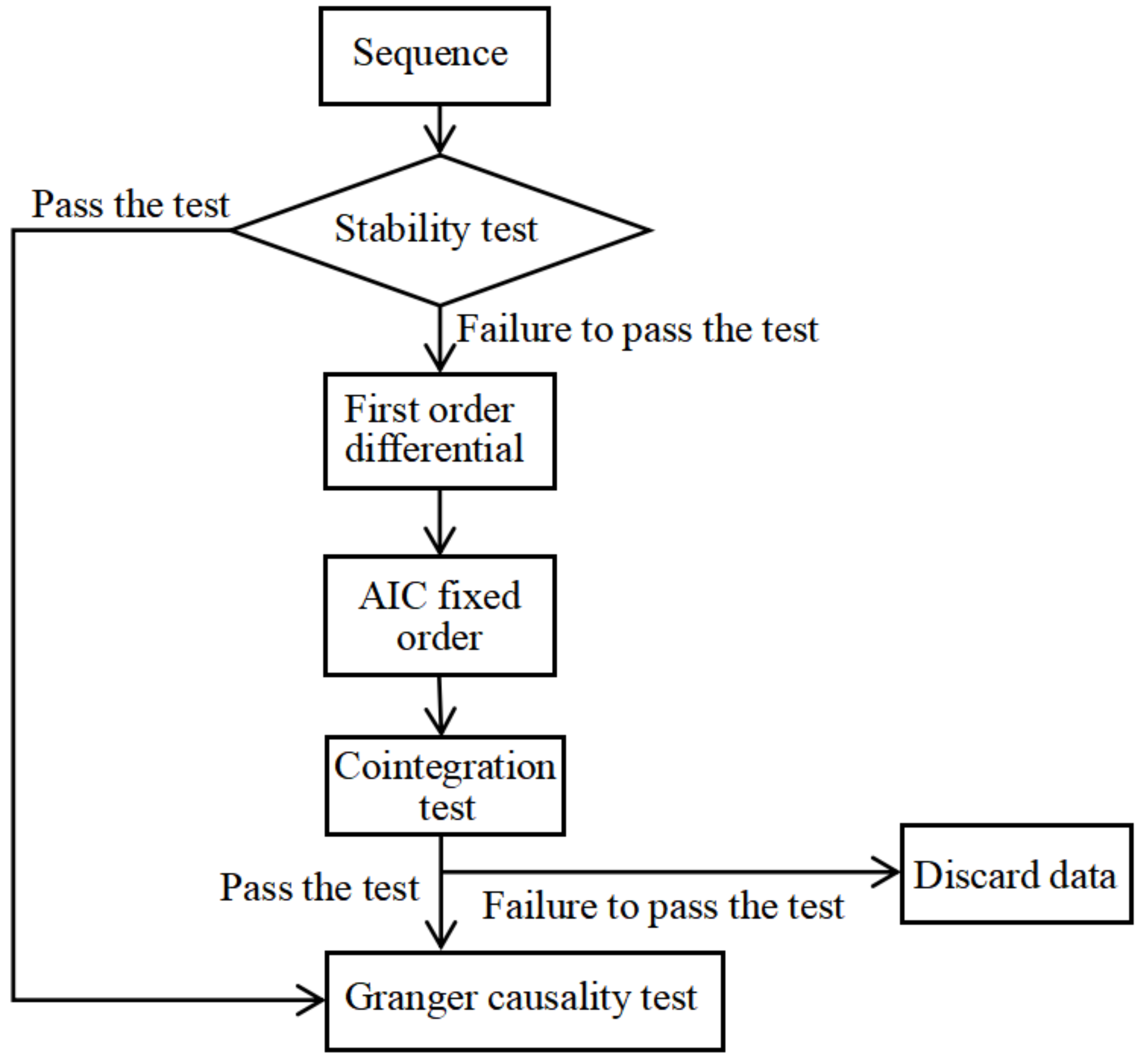
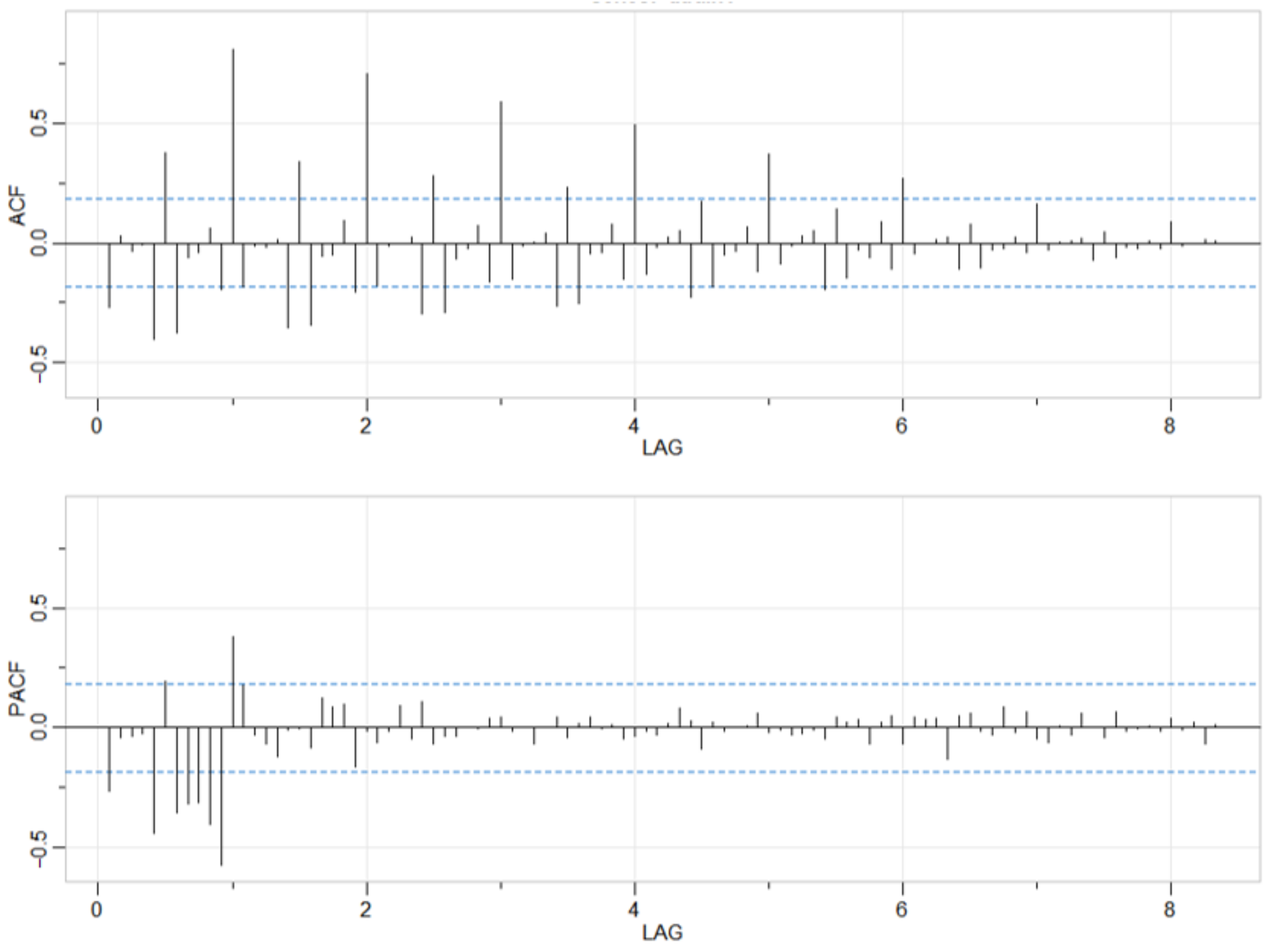
2.2.1. Multi-Feature Selection

To reduce the model training time cost and to remove meteorological variables that have little influence on the typhoon path, the meteorological variables in the forecast factors are selected using Granger causality tests to achieve data dimensionality reduction before inputting the data into the forecast model. The process of Granger causality test is shown in Figure 3.
In a time series, for two variables X and Y, variable X is considered to be the Granger cause of variable Y if variable X contributes to the prediction of variable Y and variable Y cannot explain future changes in variable X [26]. This causal relationship defined from a forecasting perspective is called the Granger relationship.
  • Stability test.
Because an important prerequisite for the Granger causality test is that the time series must be smooth, before the Granger causality test, the time series needs to be tested for smoothness by unit root test, the common test method is the Augmented Dickey–Fuller test (ADF). If the series passes the ADF test, the Granger causality test can be performed. If the series does not pass the ADF test, it needs to be differenced until all series obey the same order of single integer to further confirm whether there is a cointegration relationship between the variables.
The original hypothesis of the ADF test implies that the series is not stable when there is a unit root in the series. The series is stable only when the p-value is significantly smaller than the confidence level (1%), i.e., the original hypothesis is rejected. That is, when p < 0.01, the series is stable, and the Granger causality test can be performed. Otherwise, the first-order difference is required.
The irrelevant variables of the dataset were removed, such as year, typhoon name, etc., and finally, all meteorological variables were obtained, containing 18 variables in total, and their smoothness test results are shown in Table 3.
From Table 3, we can find that there are 12 series whose p-values are all less than 0.01, i.e., these 12 series have no unit root, are stable, and can be tested for Granger causality. While the p-values of PRES, R_LONG, R_SHORT, POCI, EYE, and GUSTS are all greater than 0.01, i.e., these 6 series are not stable and need to be first first-order differenced, i.e., using autoregression to extract the series determination information, and then test the smoothness. After the first-order differencing, the p-values of the above six series are all less than 0.01, i.e., the series is stable.
2.
Cointegration test.
After ensuring that all series are smooth, before conducting the Granger causality test, to check whether there is a cointegration relationship among the series and prevent the phenomenon of pseudo-regression, it is also necessary to conduct a cointegration test for the series with a first-order difference.
(1) The optimal lag order is selected based on the minimum criterion of the Akaike information criterion (AIC) [27]. The AIC is calculated as Equation (5).
AIC = 2 l a g + n ln R S S n
where l a g denotes the lag order, n denotes the sequence length, and R S S denotes the fit residuals.
Usually, Autocorrelation Coefficient Function (ACF) and Partial Autocorrelation Coefficient Function (PACF) can be used for ranking. In addition, automatic orderings can be performed using programming languages.
For a series x t , ACF can be used to measure the correlation between x t and x t k , while PACF can be used to measure the correlation between x t and x t k with the lagged effect of x t 1 , x t 2 , , x t k + 1 removed. Taking the weather variable CAT in the dataset as an example, its ACF plot and PACF plot outputs are shown in Figure 4.
(2) Test the stationarity of the residuals. If the residuals pass the ADF test, the series is cointegrated. Otherwise, it is not cointegrated.
In this paper, the auto.arima() function of R language was used for automatic order determination. After determining the optimal lag order, the model was constructed for the six series that were smooth only after the first-order difference, and the residuals were tested separately by the ADF test, and it was found that their p-values were all less than 0.01, i.e., all these six series had cointegration relationship, and they could be tested for Granger causality.
3.
Granger causality test.
To determine whether the above 18 meteorological variables affect the typhoon path, we need to test whether there is Granger causality between each meteorological variable and typhoon longitude and latitude in turn.
(1) Test the hypothesis “H0: X is not a Granger cause of Y change”. The two regression equations in Equations (6) and (7) are first estimated.
Unconstrained regression Equation u :
Y t = α 0 + i = 1 p α i Y t 1 + i = 1 q β i X t 1 + ε t
Constrained regression equation r :
Y t = α 0 + i = 1 p α i Y t 1 + ε t
where α 0 denotes the constant term, p and q denote the maximum lag order of variables X and Y, respectively, and ε t denotes white noise.
Then, the residual sums of squares R S S u and R S S r of the above two equations are used to construct the statistic F , which is calculated as Equation (8).
F = R S S u R S S r / q R S S u / n p q 1
where n denotes the sample size. If F F α , then the original hypothesis is rejected. If F < F α , then the original hypothesis cannot be rejected.
(2) Repeat step (1) by swapping the positions of variables Y and X. Test the hypothesis “H0: Y is not the Granger cause of the change in X”.
(3) When the hypothesis “H0: Y is not the Granger cause of the change in X” is valid and the hypothesis “H0: X is not the Granger cause of the change in Y” is not valid, we can obtain the conclusion that “variable X is the Granger cause of variable Y” is obtained when both the assumptions “H0: Y is not the Granger cause of X” and “H0: X is not the Granger cause of Y” are satisfied.
In this paper, the lag period is set to 2, and the original hypothesis indicates that this meteorological variable is not the Granger cause of typhoon latitude and longitude, which F is obtained as shown in Table 4.
When the value of F is significantly smaller than the confidence level (1%), i.e., when F < 0.01 , the original hypothesis is rejected, and this meteorological variable is the Granger cause of typhoon longitude and latitude.
Therefore, the meteorological variables DIST2LAND, LANDFALL, WIND, SPEED, and DIR are the Granger causes of typhoon longitude. The meteorological variables CAT, WIND, PRES, and DIR are the Granger causes of typhoon latitude.

2.2.2. Model

Considering the data consisting of the latitude and longitude where the typhoon center is located under different moments, i.e., the typhoon path, and the meteorological variables affecting its path are time-series in nature, and there are more meteorological variables. While CNN can extract the implicit features of multiple variables in the dataset and improve the generalization ability, LSTM can learn temporal features and improve the efficiency of the model in dealing with time series problems. Therefore, this experiment combines the two neural networks to propose a new C-LSTM network and use it for the prediction of typhoon paths.
The C-LSTM model takes as input the typhoon path and the 7 meteorological variables selected by the Granger causality test. The data set is grouped by typhoon number, and the maximum length of each typhoon sequence is set to 20 data. When the sequence length of a typhoon exceeds 20, the excess is deleted. When the sequence length of a typhoon is less than 20, it is filled with zeros. Every 5 data in each group is a matrix, and the subsequent matrices are determined using the sliding window method. The matrix of this time series format is shown in Equation (9).
M = l a t i , t 1 l o n i , t 1 F i , t 1 l a t i , t 2 l o n i , t 2 F i , t 2 l a t i , t 5 l o n i , t 5 F i , t 5
where F = f 1 , f 2 , f 7 denotes the 7 meteorological variables selected by the Granger causality test.
Then two convolutional layers were set up for extracting the feature vectors, the numbers of output channels were both 2. A Dropout layer was also added to prevent overfitting, and the LeakyReLU function was used for the start function. The output results of the CNN layer are then leveled, and the leveled results are input to the LSTM layer, which is used to learn temporal features and output the typhoon location (longitude and latitude) for the next time stamp.

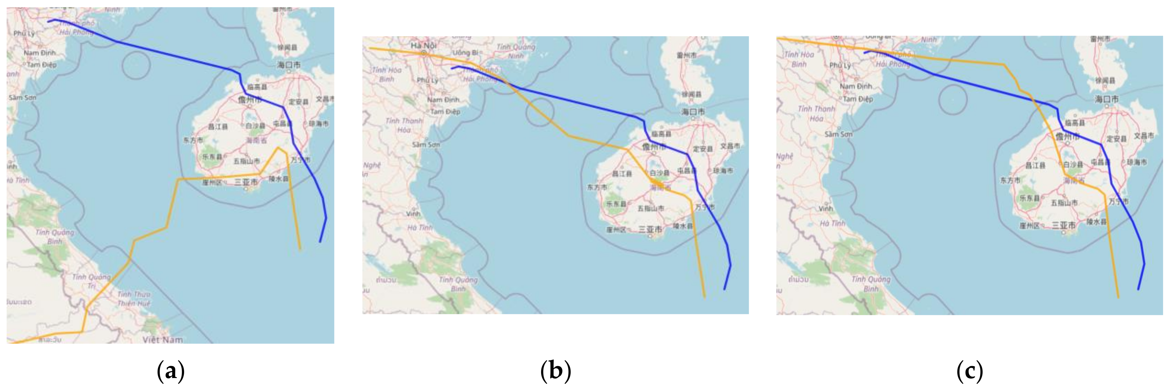
3. Experiment Results and Analysis

To verify the accuracy of the model, the typhoon path data and selected meteorological variables data in the best path data set of typhoons in the South China Sea from 1949 to 2006 were used as the training set for the typhoon path data and selected meteorological variables data from 2007 to 2020 were used as the test set, and the typhoon path data and selected meteorological variables data were used as the validation set, and some experiments were conducted to predict the typhoon paths.

3.1. Number of Iterations Level

In this experiment, the performance of the model is compared at the level of the number of iterations based on the loss results of the C-LSTM-based typhoon path prediction model with a different number of iterations. In this experiment, the number of iterations of the C-LSTM-based typhoon path prediction model is set to 25, 50, and 100, respectively, and the obtained loss variation of the training set is shown in Figure 5.
From Figure 5, we can see that the loss value of the model keeps converging as the number of iterations increases. When the number of iterations is 25, the loss of the training set is 321.94, and the loss of the test set is 213.45. When the number of iterations is 50, the loss of the training set is 140.82, and the loss of the test set is 102.46. When the number of iterations is 100, the loss of the training set is 139.28, and the loss of the test set is 101.902. Moreover, when the number of iterations increases from 50 to 100 iterations, although the time required increases, i.e., the time cost increases, the value of its loss decrease is smaller, so the case of iterations greater than 100 iterations is not considered again.
In addition, to see the error between the prediction results and the real path of the typhoon based on the C-LSTM typhoon path prediction model with a different number of iterations, this paper takes the typhoon “Lionrock” in 2021 as an example and calls the folium library in Python to plot the predicted path and the actual path on a world map. In this paper, the predicted path and the actual path are plotted on the world map by calling the folium library in Python, and the typhoon path is visualized in Figure 6, in which the blue path represents the real path of the typhoon, and the orange path represents the predicted path of the typhoon by using the C-LSTM model.
From Figure 6, we can see that when the number of iterations increases, the predicted path of the typhoon and the real path of the typhoon, though there is always a certain error, gradually converge in the same general direction. For this typhoon, the surface distance error is used as the evaluation index to calculate the average surface distance error between the two, which is calculated as shown in Equation (10).
Δ d = Δ x 2 + Δ y 2 × Δ s
where Δ x and Δ y denote the longitude error and latitude error of the typhoon path prediction results, respectively, and Δ s denotes the distance between the predicted longitude and latitude of the typhoon path and the actual longitude and latitude of the typhoon path [28], whose specific expression is shown in Equation (11).
Δ s = R × arccos sin φ 1 sin φ 2 + cos φ 1 cos φ 2 cos λ 1 λ 2
where R denotes the radius of the earth, generally taken as 6371 km, and φ 1 and λ 1 denote the longitude and latitude of the i th point, respectively.
When the number of iterations is 25, its average surface distance error has 56,326 m. When the number of iterations is 50, its average surface distance error has 10,621 m. When the number of iterations is 100, its average surface distance error is only 832 m. That is, when the number of iterations is 100, its average surface distance error is the smallest, and the prediction accuracy is the highest.

3.2. Comparison Experiments Level

To show more intuitively whether the performance of the C-LSTM model proposed in this experiment is improved compared with the existing prediction models, a typhoon path prediction model based on LSTM is also constructed for comparison in this experiment. To better form a control experiment, the same data set, and parameters are used for this model and the C-LSTM model.
In this experiment, the LSTM model is constructed to compare with the C-LSTM model, and the model parameters are adjusted by adjusting the loss function and optimizer to select the optimal parameters for the model.
Because in the above experiments, the loss is the smallest and the best when the number of iterations is 100, the number of iterations of each model is also set to 100 in this comparison experiment to facilitate the comparison of the prediction results. The prediction results of the two models using the surface distance error as the evaluation index with different parameter choices when the number of iterations is set to 100 are shown in Table 5.
Through the experimental results in Table 5, we can see that the average surface distance errors of the C-LSTM-based typhoon path prediction models are all smaller than those of the LSTM-based typhoon path prediction models. This is probably because the CNN layer in the C-LSTM-based typhoon path prediction model allows the model to learn the features of the input data better, thus improving the model prediction accuracy. Moreover, we can see that the model with cross-entropy loss function and Adam optimizer performs the best among several C-LSTM-based typhoon path prediction models.
To compare the errors between the C-LSTM typhoon path prediction model and the LSTM typhoon path prediction model and the real path of the typhoon, the comparison experiment also chose the typhoon “Lionrock” which will make landfall in 2021 as an example. The comparison experiment also chooses to take the typhoon “Lionrock” that will make landfall in 2021 as an example and plots its predicted path and the actual path on the world map for visualization. The specific comparison between the two models is shown in Figure 7, where the blue path indicates the real path of the typhoon, while the orange path represents the corresponding typhoon path predicted using the two different models.
From Figure 7, we can see that although there are some errors between the predicted and true paths of the typhoon obtained by these two prediction models, they are generally consistent in terms of the general direction. For this typhoon, by using the surface distance error as the evaluation index and calculating the average surface distance error between them, we can get the average surface distance error between the predicted path and the true path obtained by the LSTM typhoon path prediction model is 11,503 m. The average surface distance error between the predicted path and the true path obtained by the C-LSTM typhoon path prediction model proposed in this paper is only 832 m. The average surface distance error between the predicted path and the real path is only 832 m.

4. Conclusions

In this paper, typhoons originating in the South China Sea are studied for the typhoon track prediction problem. In this paper, a C-LSTM typhoon path prediction model is constructed to form a dataset using typhoon paths and related meteorological variables formed in the South China Sea from 1949 to 2021, and a Granger causality test is used to select multiple features for the dataset before inputting it into the prediction model to realize data dimensionality reduction. In addition, a prediction model based on the LSTM network was constructed for comparison experiments. The final experimental results show that the C-LSTM-based typhoon path prediction model outperforms the LSTM-based typhoon path prediction model, and it works best when the cross-entropy loss function and Adam optimizer are selected, and its average surface distance error is only about 14.66 km.
Although the feasibility of the C-LSTM-based typhoon path prediction model proposed in this paper is proved through experiments, it still has some limitations and can be optimized further. First, since the causes and triggering mechanisms of typhoons are still unclear and the factors affecting typhoon paths are uncertain, the relationship between typhoon activity and meteorological changes can be further explored in the follow-up. Second, only the South China Sea typhoon data in the best path data set of the Northwest Pacific typhoon were used in this paper, and the influence of typhoon intensity decay on typhoon path and disappearance time was not considered. In the future, we can consider using other existing public data, and we can also consider combining image data and numerical data, or even using the data set obtained by fusing multiple observation methods for typhoon path prediction. That is, the effectiveness and accuracy of forecasts can be improved by increasing the diversity of data and the amount of data used for forecasting. Third, this paper sets up fewer comparative experiments and constructs only one model based on C-LSTM, after which we can try to construct deeper neural network models or build models for typhoon path prediction by combining several other neural networks.

Author Contributions

N.X. wrote the manuscript; J.R. and N.X. collected the data; Y.C. and J.R. edited and revised the manuscript; N.X. drew the figures; N.X. and J.R. designed research methods; N.X. analyzed the data; J.R. project administration; J.R. and Y.C. funding acquisition. All authors have read and agreed to the published version of the manuscript.

Funding

This work is supported by the High-level Talent Project of Hainan Provincial Natural Science Foundation (620RC557); Hainan Provincial Natural Science Foundation Innovation Research Team Project (620CXTD434); National Natural Science Foundation of China and Macau Science and Technology Development Joint Fund (61961160706 and 0066/2019/AFJ); the Hainan Provincial Key R & D Plan (ZDYF2021GXJS199).

Data Availability Statement

Data are contained within the article. The data presented in this study can be requested from the authors.

Conflicts of Interest

The authors declare no conflict of interest.

References

  1. Wang, X.Y. A synthesis of traditional models and neural networks for predicting typhoon tracks. Sci. Advis. (Sci. Technol.—Manag.) 2020, 4, 62–65. [Google Scholar]
  2. Liu, Y.D.; Wang, B.; Hou, Z.M. Application of the Optimal Decision Method to Typhoon Track Forecasting. J. Trop. Meteorol. 2003, 19, 219–224. [Google Scholar]
  3. Zou, J.P. Analysis of Typhoon “Rammasu” rainstorm in central and western Hainan Province. Mod. Agric. Sci. Technol. 2017, 24, 209–210. [Google Scholar]
  4. Burpee, R.W. The Sanders Barotropic Tropical Cyclone Track Prediction Model (SANBAR). Meteorol. Monogr. 2008, 33, 233–240. [Google Scholar] [CrossRef]
  5. Chen, Z.T.; Dai, G.F.; Luo, Q.H.; Zhong, S.X.; Zhang, Y.X.; Dao-Sheng, X.U.; Huang, Y.Y. Study on the Coupling of Model Dynamics and Physical Processes and Its Influence on the Forecast of Typhoons. J. Trop. Meteorol. 2016, 32. [Google Scholar] [CrossRef]
  6. Yang, C.; Min, J.; Liu, Z. Technology, The Impact of AMSR2 Radiance Data Assimilation on the Analysis and Forecast of Typhoon Son-Tinh. Chin. J. Atmos. Sci. 2017, 41, 13. [Google Scholar] [CrossRef]
  7. Neumann, C.J. An Alternate to the HURRAN (Hurricane Analog) Tropical Cyclone Forecast System; Scientific Services Division: Fort Worth, TX, USA, 1972. [Google Scholar]
  8. Liao, M.; Huang, L.; Hu, J. CLIPER Model of Track Prediction for Typhoons over the Northwestern Pacific on the Occasion of Shipping. Navig. China 1996, 43–50. [Google Scholar]
  9. Hu, J.; Chang, M.; Huang, L.; Liao, M. The CLIPER Models for Predicting Tracks of the South China Sea Typhoon. Trans. Oceanol. Limnol. 1994, 11, 191–201. [Google Scholar]
  10. Huang, L.; Liao, M.; Hu, J. CLIPER Model of Prediction for Tracks of Typhoon over the East China Sea. Mar. Forecast. 1994, 11, 12. [Google Scholar]
  11. Xiong, X.; Kai, Y.U.; Xiao, K. Prediction of Typhoon Path Based on Weather Similarity Condition. J. Geomat. 2017, 42, 3. [Google Scholar]
  12. Huo, Z.; Duan, W. The application of the orthogonal conditional nonlinear optimal perturbations method to typhoon track ensemble forecasts. Sci. China Earth Sci. 2019, 62, 376–388. [Google Scholar] [CrossRef]
  13. Song, H.J.; Huh, S.H.; Kim, J.H.; Ho, C.H.; Park, S.K. Typhoon Track Prediction by a Support Vector Machine Using Data Reduction Methods. In Proceedings of the International Conference on Computational and Information Science, Xi’an, China, 15–19 December 2005. [Google Scholar]
  14. Huang, X.Y.; Long, J.; Shi, X.M. A Nonlinear Artificial Intelligence Ensemble Prediction Model Based on EOF for Typhoon Track. In Proceedings of the 2011 Fourth International Joint Conference on Computational Sciences and Optimization, Kunming/Lijiang, China, 15–19 April 2011. [Google Scholar]
  15. Kim, H.S.; Kim, J.H.; Ho, C.H.; Chu, P.S. Pattern classification of typhoon tracks using fuzzy c-means clustering method and related large-scale circulations. Proc. Korean Meteorol. Soc. Conf. 2010, 4, 171. [Google Scholar]
  16. Tan, J.; Chen, S.; Wang, J. Western North Pacific tropical cyclone track forecasts by a machine learning model. Stoch. Environ. Res. Risk Assess. 2021, 35, 1113–1126. [Google Scholar] [CrossRef]
  17. Kovordanyi, R.; Roy, C. Cyclone track forecasting based on satellite images using artificial neural networks. ISPRS J. Photogramm. Remote Sens. 2009, 64, 513–521. [Google Scholar] [CrossRef]
  18. Shao, L.M.; Fu, G.; Chao, X.C.; Zhou, J. Application of BP neural network to forecasting typhoon tracks. J. Nat. Disasters 2009, 18, 104–111. [Google Scholar]
  19. Gao, S.; Zhao, P.; Pan, B.; Li, Y.; Zhou, M.; Xu, J.; Zhong, S.; Shi, Z. A nowcasting model for the prediction of typhoon tracks based on a long short term memory neural network. Acta Oceanol. Sin. 2018, 37, 12–16. [Google Scholar] [CrossRef]
  20. Kerh, T.; Wu, S.H. Nonlinear Autoregressive Network with the Use of a Moving Average Method for Forecasting Typhoon Tracks. Int. J. Artif. Intell. Appl. 2017, 8, 57–71. [Google Scholar] [CrossRef]
  21. Xu, G.; Zheng, H.; Huang, G.; Wu, F.; Mathematics, S.O.; University, S.J. Typhoon Track Prediction Based on Gated Recurrent Unit Neural Network. Comput. Appl. Softw. 2019, 36, 7. [Google Scholar]
  22. Sophie, G.R.; Mo, Y.; Guillaume, C.; Christina, K.B.; Balázs, K.; Claire, M. Tropical Cyclone Track Forecasting Using Fused Deep Learning from Aligned Reanalysis Data. Front. Big Data 2020, 3, 1. [Google Scholar]
  23. Sun, Y.; Song, Y.; Qiao, B.; Li, B. Distributed Typhoon Track Prediction Based on Complex Features and Multitask Learning. Complexity 2021, 2021, 5661292. [Google Scholar] [CrossRef]
  24. Mario, R.; Sangseung, L.; Soohwan, J.; Donghyun, Y. Prediction of a typhoon track using a generative adversarial network and satellite images. Sci. Rep. 2019, 9, 6057. [Google Scholar]
  25. Willmott, C.J.; Matsuura, K. Advantages of the mean absolute error (MAE) over the root mean square error (RMSE) in assessing average model performance. Clim. Res. 2005, 30, 79–82. [Google Scholar] [CrossRef]
  26. Bates, J.M.; Granger, C. The Combination of Forecasts. J. Oper. Res. Soc. 1969, 20, 451–468. [Google Scholar] [CrossRef]
  27. Akaike, H. A new look at the statistical model identification. IEEE Trans. Autom. Control. 1974, 19, 716–723. [Google Scholar] [CrossRef]
  28. Huang, S.Y.; Jin, L.; Yao, C.; Huang, M.C. An Objective Forecasting Method for the Movement Path of Typhoons in the South China Sea in Summer. J. Nanjing Meteorol. Inst. 2008, 31, 287–292. [Google Scholar]
Figure 1. Frequency of natural disasters and direct economic losses in Hainan Province, 2014–2019.
Applsci 12 08028 g001
Figure 2. The data type of each data in the dataset.
Applsci 12 08028 g002
Figure 3. Process of Granger causality test.
Applsci 12 08028 g003
Figure 4. ACF and PACF plots of the meteorological variable CAT.
Applsci 12 08028 g004
Figure 5. Losses of the C-LSTM model with selected cross-entropy loss functions and Adam optimizer for a different number of iterations. (a) The loss when the number of iterations is 25, (b) the loss when the number of iterations is 50, (c) the loss when the number of iterations is 100.
Applsci 12 08028 g005
Figure 6. Comparison of the real and predicted paths of Typhoon “Lionrock” under different iterations, where the blue path indicates the actual path of the typhoon and the orange path indicates the path predicted by the model. (a) The path comparison when the number of iterations is 25, (b) the path comparison when the number of iterations is 50, (c) the path comparison when the number of iterations is 100. p.s. The left side of the ocean represents Vietnam, where the non-English text indicates different cities in Vietnam; the right side of the ocean represents Hainan, China, where the non-English text indicates different cities in China.
Applsci 12 08028 g006
Figure 7. Comparison of the predicted path of Typhoon “Lionrock” using two models, where the blue path indicates the actual path of the typhoon and the orange path indicates the path predicted by different models. (a) The comparison of the true path and predicted path using the LSTM model for prediction, (b) the comparison of the true path and predicted path using the C-LSTM model for prediction. p.s. The left side of the ocean represents Vietnam, where the non-English text indicates different cities in Vietnam; the right side of the ocean represents Hainan, China, where the non-English text indicates different cities in China.
Applsci 12 08028 g007
Table 1. The specific composition of the best path data set for South China Sea typhoons.
Variable NameDescriptionVariable NameDescription
SIDTropical cyclone numberBASINOcean area code where the typhoon center is located, WP Northwest Pacific region
SEASONYear
NUMBERThe base number of the system
IFLAGIdentifies the observation point that provides data at the current momentGUSTSMaximum instantaneous wind speed near the center (i.e., gust). Unit: knot
WINDMaximum sustained wind speed at the current moment. Unit: knotR_DIRThe direction of the quadrant corresponds to the radius.
NE-Northeast, SE-Southeast, SW-Southwest, NW-Northwest
PRESMinimum sea level pressure. Unit: hPa
SUBREGIONSub-region code where the typhoon center is locatedR_LONGThe radius of maximum wind. Unit: nm
NAMEInternational name of the typhoonR_SHORTMinimum wind radius. Unit: nm
ISO_TIMEISO format time. Recorded at 3-h intervalsTRACK_TYPETrack type
CATcyclone nature or category.
DS-disturbance, TS-tropical storm, SS-subtropical storm, ET-extrapolation, NR-unreported, MM-mixed (conflicting reports among multiple agencies)
SPEEDThe speed at which the center of a typhoon moves. Unit: knot
DIRThe direction of movement of the typhoon center. Unit: °
EYEThe diameter of the wind eye. Unit: nm
LATLatitude at which the typhoon is currently locatedLONCurrent longitude of the typhoon
LANDFALLUsed to determine whether landfall is possible within 6 hPOCIOutermost isobaric pressure (i.e., outer pressure). Unit: hPa
DIST2LANDDistance from the current position to the nearest land. Unit: kmROCIRadius of outermost isobar. Unit: nm
Table 2. Error evaluation results for missing fill.
Meteorological VariablesWINDPRESROCIEYE
RMSE0.0350810.036410.036940.03589
Table 3. The results of smoothness tests of typhoon meteorological variables.
Meteorological Variablesp-ValueMeteorological Variablesp-Value
CAT<0.01R_LONG0.06493
LAT<0.01R_SHORT0.08179
LON<0.01POCI0.6398
TRACK_TYPE<0.01ROCI<0.01
DIST2LAND<0.01RMW<0.01
LANDFALL<0.01EYE0.03763
WIND<0.01GUSTS0.4172
PRES0.5646SPEED<0.01
R_DIR<0.01DIR<0.01
Table 4. Pairwise results of Granger causality tests between meteorological variables and typhoon paths (longitude, latitude).
Meteorological Variablesp-Value (lon)p-Value (lat)Meteorological Variablesp-Value (lon)p-Value (lat)
CAT<1<0.001R_SHORT<1<0.05
TRACK_TYPE<0.05<1POCI<1<0.05
DIST2LAND<0.001<0.05ROCI<1<1
LANDFALL<0.001<0.1RMW<1<1
WIND<0.001<0.001EYE<1<1
PRES<0.1<0.001GUSTS<0.05<1
R_DIR<0.05<0.1SPEED<0.001<1
R_LONG<1<0.1DIR<0.001<0.001
Table 5. Average surface distance error between predicted and real paths with different parameters of the C-LSTM model and LSTM model (unit: km).
Model StructureAverage Surface Distance Error (km)
C-LSTM + MSE + AdamTraining set19.795
Test set20.651
Validation set20.232
C-LSTM + cross-entropy loss function + AdamTraining set14.215
Test set14.291
Validation set15.487
C-LSTM + cross-entropy loss function + SGDTraining set20.716
Test set21.623
Validation set21.303
LSTM + MSE + AdamTraining set23.999
Test set24.15
Validation set23.546
LSTM + cross-entropy loss function + AdamTraining set22.69
Test set23.981
Validation set22.011
LSTM + cross-entropy loss function + SGDTraining set37.0865
Test set37.289
Validation set37.44
Publisher’s Note: MDPI stays neutral with regard to jurisdictional claims in published maps and institutional affiliations.

