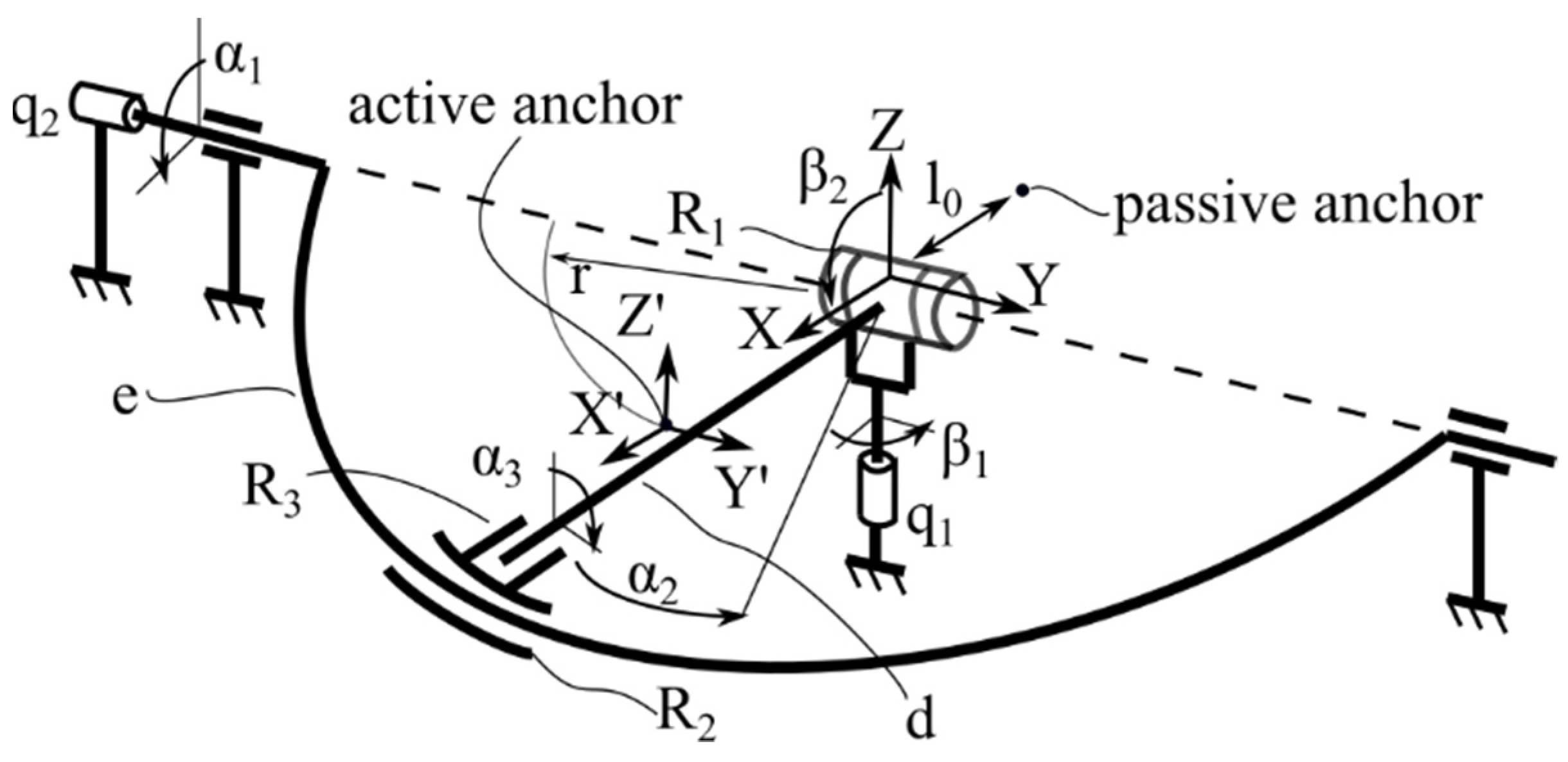
Figure 1.
The ParReEx-wrist kinematic scheme [
47].
Figure 1.
The ParReEx-wrist kinematic scheme [
47].
Figure 2.
The ParReEx-wrist CAD model.
Figure 2.
The ParReEx-wrist CAD model.
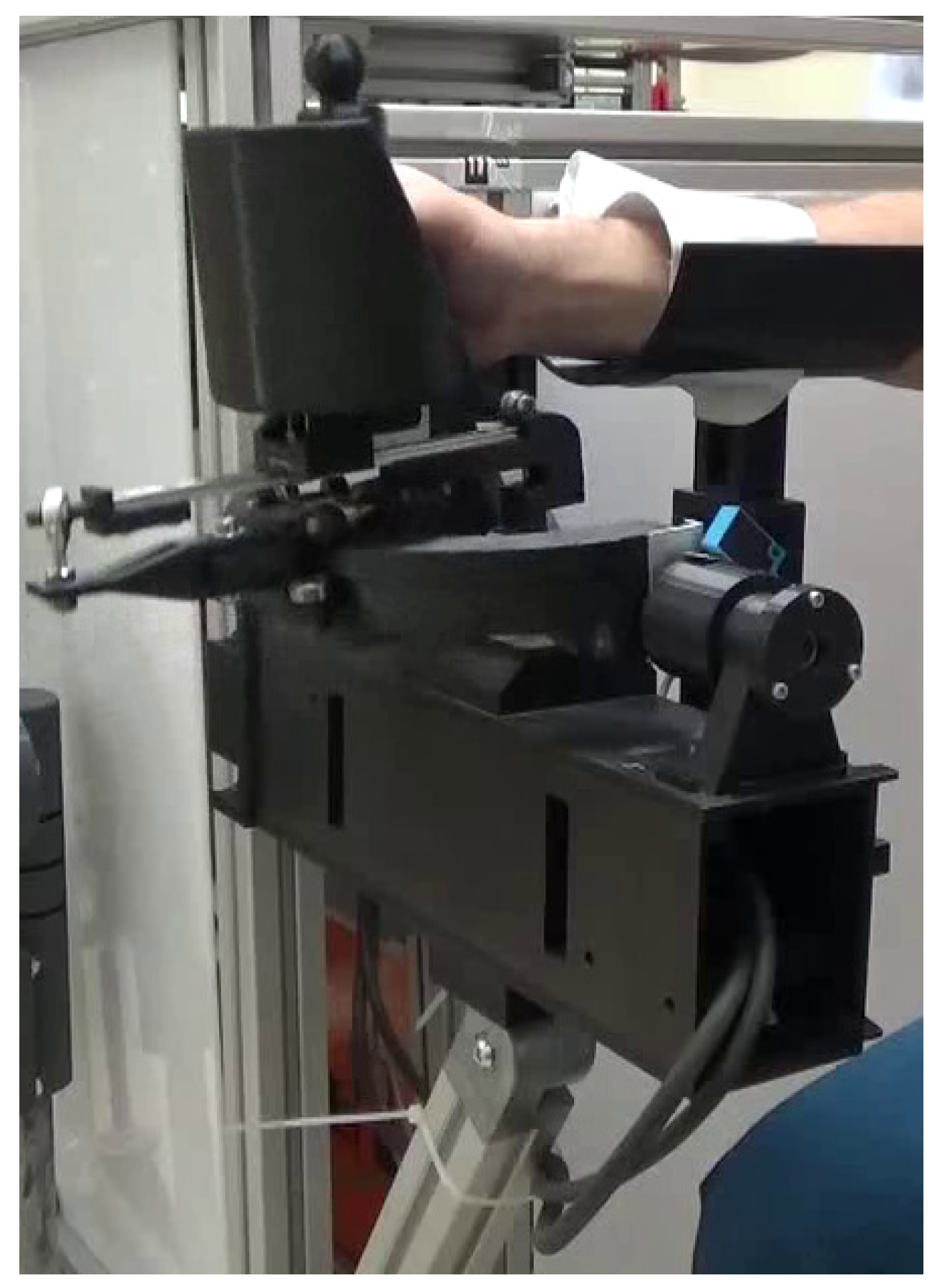
Figure 3.
The ParReEx-wrist experimental model.
Figure 3.
The ParReEx-wrist experimental model.
Figure 4.
Kinematic joints defined in the ADAMS dynamic model.
Figure 4.
Kinematic joints defined in the ADAMS dynamic model.
Figure 5.
Law of motion imposed in ADAMS on ParReEx-wrist robot motor Joint E.
Figure 5.
Law of motion imposed in ADAMS on ParReEx-wrist robot motor Joint E.
Figure 6.
The two extreme positions during the operation of the virtual model of the ParReEx-wrist robot, corresponding to combined flexion–extension and radial–ulnar motion.
Figure 6.
The two extreme positions during the operation of the virtual model of the ParReEx-wrist robot, corresponding to combined flexion–extension and radial–ulnar motion.
Figure 7.
ADAMS simulation computed torque for: (a) the flexion–extension module and (b) the radial–ulnar module.
Figure 7.
ADAMS simulation computed torque for: (a) the flexion–extension module and (b) the radial–ulnar module.
Figure 8.
Positioning of the axes of the kinematic joints of the ParReEx robot.
Figure 8.
Positioning of the axes of the kinematic joints of the ParReEx robot.
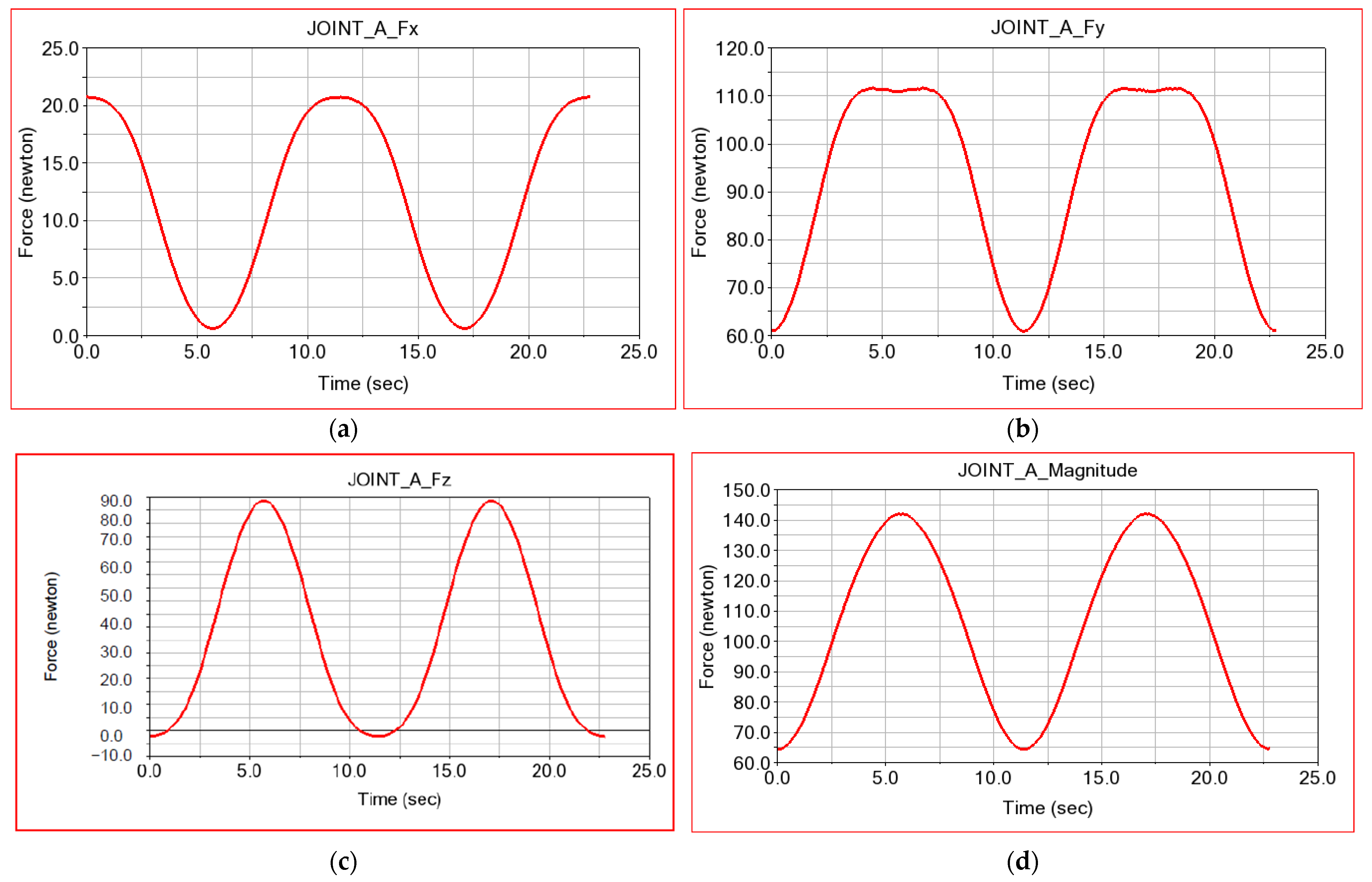
Figure 9.
Connecting forces in rotation Joint A: (a) in the x-direction; (b) in the y-direction; (c) in the z-direction; and (d) the resultant.
Figure 9.
Connecting forces in rotation Joint A: (a) in the x-direction; (b) in the y-direction; (c) in the z-direction; and (d) the resultant.
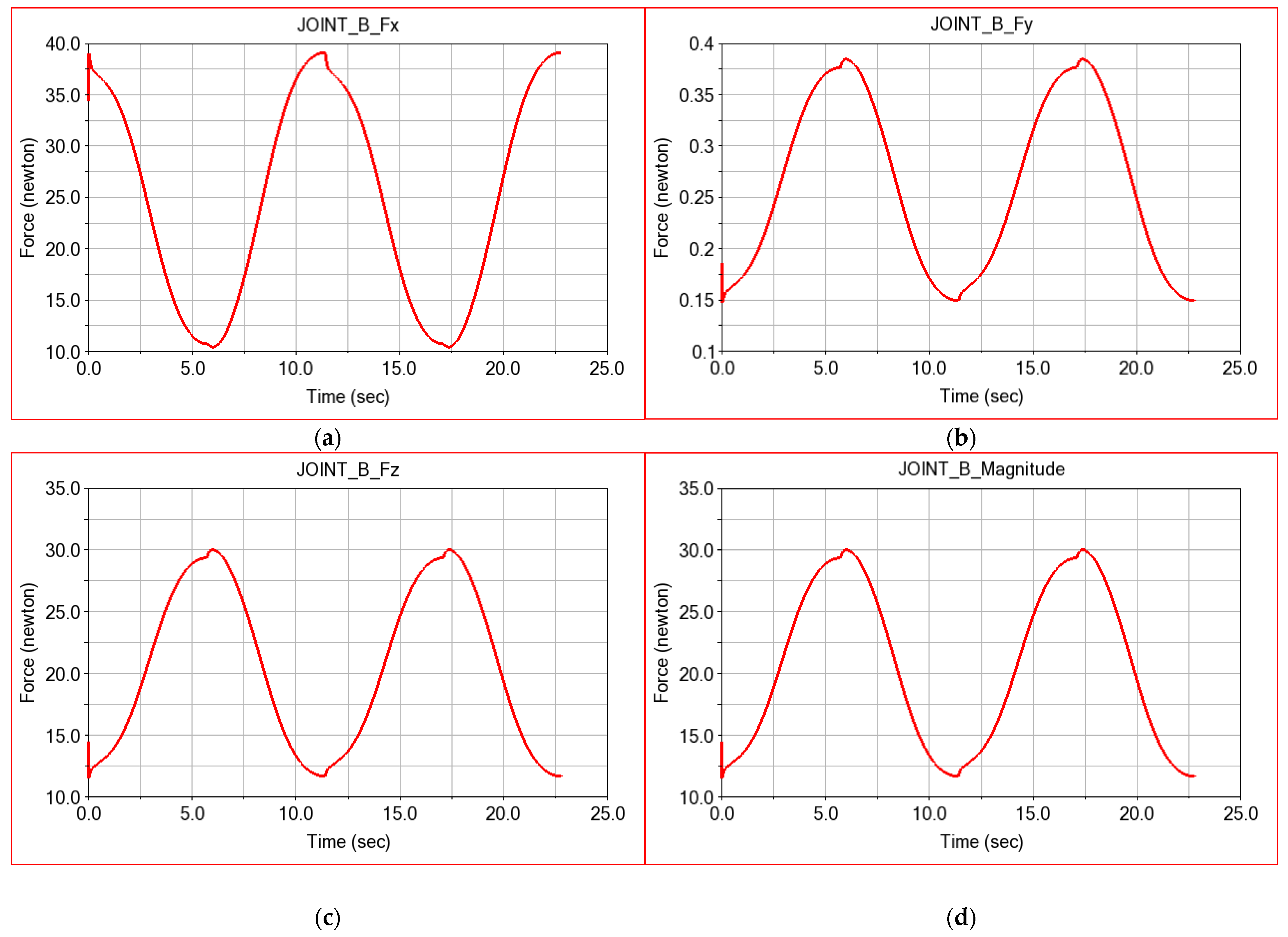
Figure 10.
Connecting forces in rotational Joint B: (a) in the x-direction; (b) in the y-direction; (c) in the z-direction; and (d) the resultant.
Figure 10.
Connecting forces in rotational Joint B: (a) in the x-direction; (b) in the y-direction; (c) in the z-direction; and (d) the resultant.
Figure 11.
Connecting forces in rotational Joint R1: (a) in the x-direction; (b) in the y-direction; (c) in the z-direction; and (d) the resultant.
Figure 11.
Connecting forces in rotational Joint R1: (a) in the x-direction; (b) in the y-direction; (c) in the z-direction; and (d) the resultant.
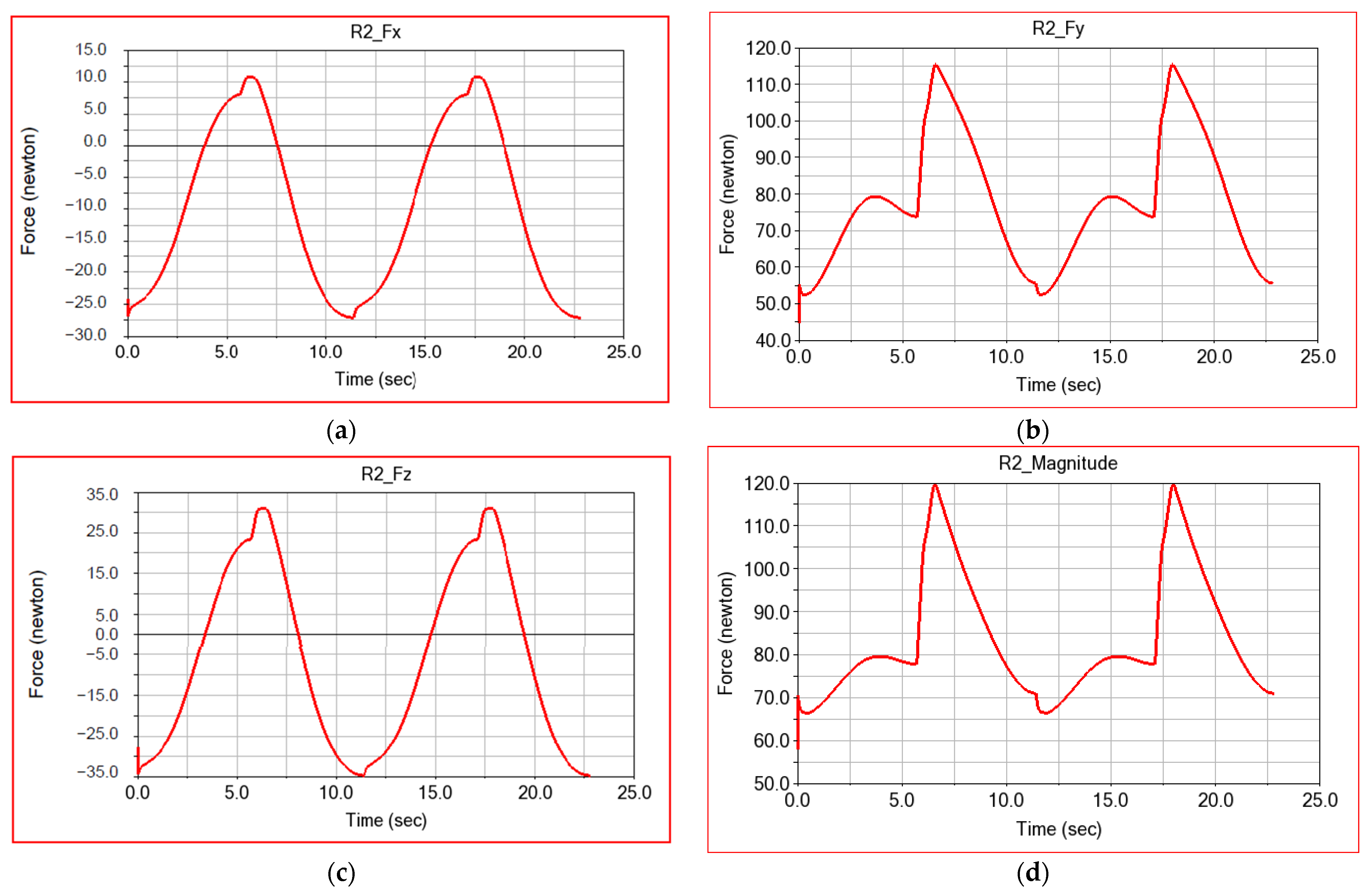
Figure 12.
Connecting forces in rotational Joint R2 of the flexion/extension module: (a) in the x-direction; (b) in the y-direction; (c) in the z-direction; and (d) the resultant.
Figure 12.
Connecting forces in rotational Joint R2 of the flexion/extension module: (a) in the x-direction; (b) in the y-direction; (c) in the z-direction; and (d) the resultant.
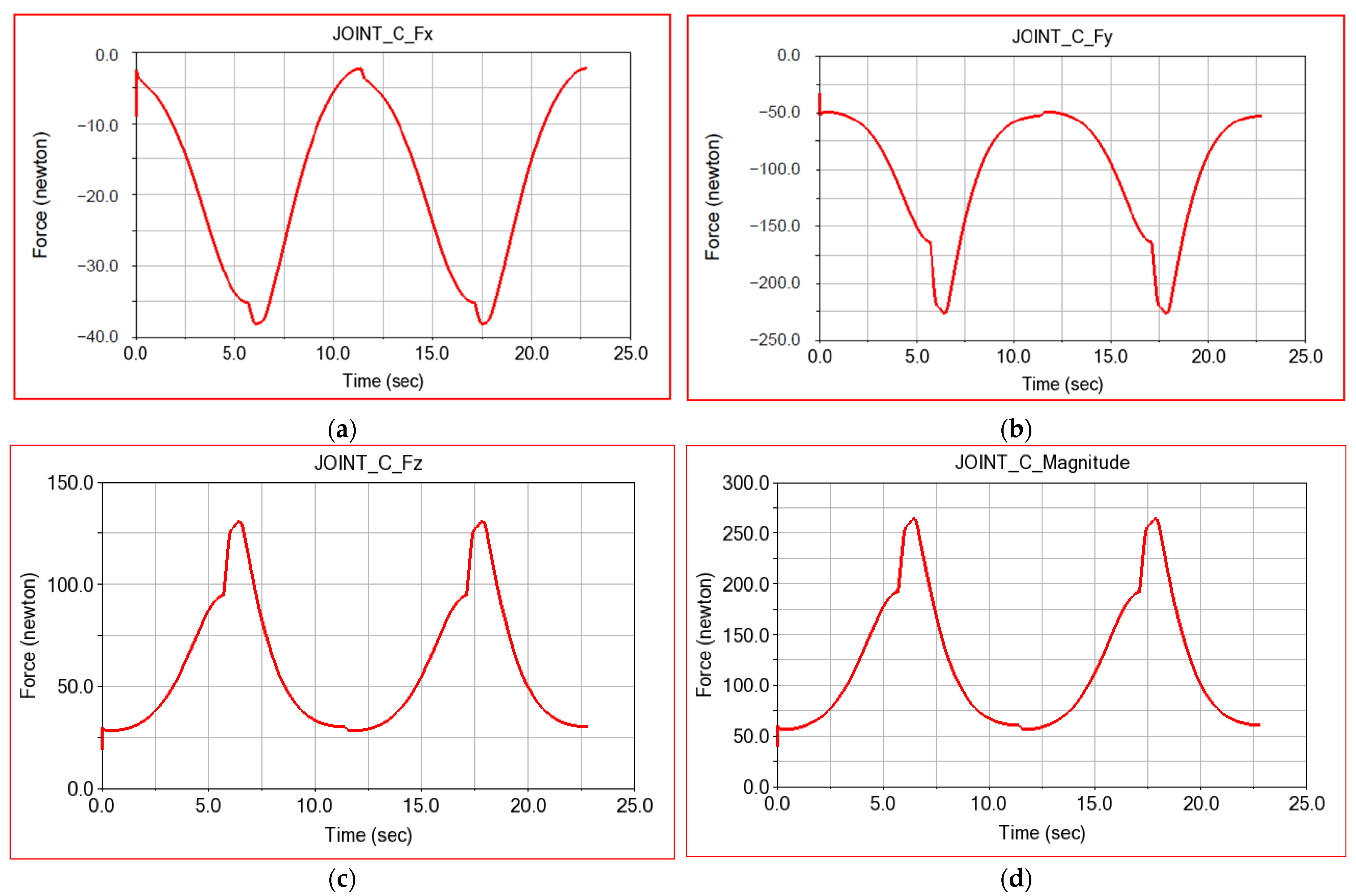
Figure 13.
Connecting forces in rotational Joint C: (a) in the x-direction; (b) in the y-direction; (c) in the z-direction; and (d) the resultant.
Figure 13.
Connecting forces in rotational Joint C: (a) in the x-direction; (b) in the y-direction; (c) in the z-direction; and (d) the resultant.
Figure 14.
Second case—ADAMS-simulation-computed torque for: (a) the flexion–extension module and (b) the radial–ulnar deviation module.
Figure 14.
Second case—ADAMS-simulation-computed torque for: (a) the flexion–extension module and (b) the radial–ulnar deviation module.
Figure 15.
Connecting forces in rotation Joint A computed with friction consideration: (a) in the x-direction; (b) in the y-direction; (c) in the z-direction; and (d) the resultant.
Figure 15.
Connecting forces in rotation Joint A computed with friction consideration: (a) in the x-direction; (b) in the y-direction; (c) in the z-direction; and (d) the resultant.
Figure 16.
Connecting forces in Joint B calculated assuming friction: (a) in the x-direction; (b) in the y-direction; (c) in the z-direction; and (d) the resultant.
Figure 16.
Connecting forces in Joint B calculated assuming friction: (a) in the x-direction; (b) in the y-direction; (c) in the z-direction; and (d) the resultant.
Figure 17.
Connecting forces in rotational Joint R1: (a) in the x-direction; (b) in the y-direction; (c) in the z-direction; and (d) the resultant.
Figure 17.
Connecting forces in rotational Joint R1: (a) in the x-direction; (b) in the y-direction; (c) in the z-direction; and (d) the resultant.
Figure 18.
Connecting forces in rotational Joint R2: (a) in the x-direction; (b) in the y-direction; (c) in the z-direction; and (d) the resultant.
Figure 18.
Connecting forces in rotational Joint R2: (a) in the x-direction; (b) in the y-direction; (c) in the z-direction; and (d) the resultant.
Figure 19.
Connecting forces in rotational Joint C: (a) in the x-direction; (b) in the y-direction; (c) in the z-direction; and (d) the resultant.
Figure 19.
Connecting forces in rotational Joint C: (a) in the x-direction; (b) in the y-direction; (c) in the z-direction; and (d) the resultant.
Figure 20.
The deformable body in ADAMS and view of body deformation map.
Figure 20.
The deformable body in ADAMS and view of body deformation map.
Figure 21.
The laws of variation of computed torque for: (a) the flexion–extension module and (b) the radial–ulnar module.
Figure 21.
The laws of variation of computed torque for: (a) the flexion–extension module and (b) the radial–ulnar module.
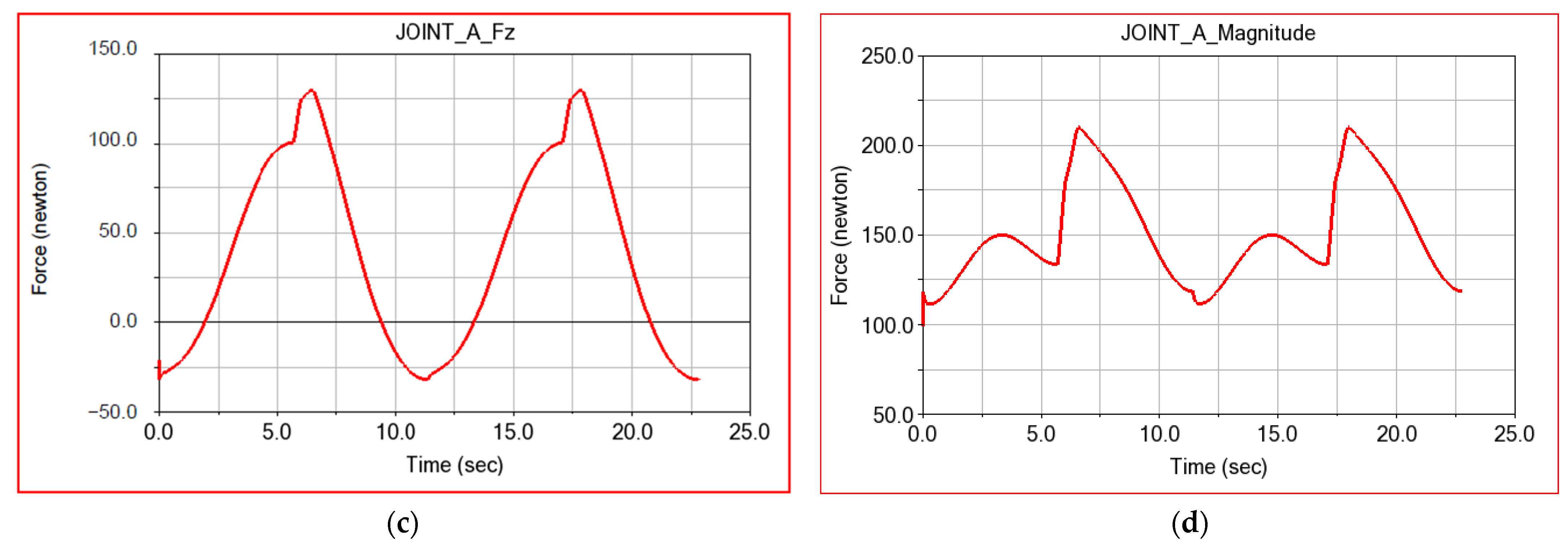
Figure 22.
Connecting forces in rotation Joint A computed with friction and flexible links: (a) in the x-direction; (b) in the y-direction; (c) in the z-direction; and (d) the resultant.
Figure 22.
Connecting forces in rotation Joint A computed with friction and flexible links: (a) in the x-direction; (b) in the y-direction; (c) in the z-direction; and (d) the resultant.
Figure 23.
Connecting forces in Joint B calculated assuming friction and flexible links: (a) in the x-direction; (b) in the y-direction; (c) in the z-direction; and (d) the resultant.
Figure 23.
Connecting forces in Joint B calculated assuming friction and flexible links: (a) in the x-direction; (b) in the y-direction; (c) in the z-direction; and (d) the resultant.
Figure 24.
Connecting forces in rotational Joint R1 in Case 3: (a) in the x-direction; (b) in the y-direction; (c) in the z-direction; and (d) the resultant.
Figure 24.
Connecting forces in rotational Joint R1 in Case 3: (a) in the x-direction; (b) in the y-direction; (c) in the z-direction; and (d) the resultant.
Figure 25.
Connecting forces in rotational Joint R2 in Case 3: (a) in the x-direction; (b) in the y-direction; (c) in the z-direction; and (d) the resultant.
Figure 25.
Connecting forces in rotational Joint R2 in Case 3: (a) in the x-direction; (b) in the y-direction; (c) in the z-direction; and (d) the resultant.
Figure 26.
Connecting forces in rotational Joint C in Case 3: (a) in the x-direction; (b) in the y-direction; (c) in the z-direction; and (d) the resultant.
Figure 26.
Connecting forces in rotational Joint C in Case 3: (a) in the x-direction; (b) in the y-direction; (c) in the z-direction; and (d) the resultant.
Figure 27.
Displacement of the center of mass of the circular guide: (a) in the x-direction; (b) in the y-direction; (c) in the z-direction; and (d) the resultant.
Figure 27.
Displacement of the center of mass of the circular guide: (a) in the x-direction; (b) in the y-direction; (c) in the z-direction; and (d) the resultant.
Figure 28.
Deformation of the center of mass of the circular guide: (a) in the x-direction; (b) in the y-direction; (c) in the z-direction; and (d) the resultant.
Figure 28.
Deformation of the center of mass of the circular guide: (a) in the x-direction; (b) in the y-direction; (c) in the z-direction; and (d) the resultant.
Figure 29.
Deformation map of the robot circular guide.
Figure 29.
Deformation map of the robot circular guide.
Figure 30.
Parameterized model of the circular guide in ANSYS Design Modeler.
Figure 30.
Parameterized model of the circular guide in ANSYS Design Modeler.
Figure 31.
Block diagram of the structural optimization process of the guide.
Figure 31.
Block diagram of the structural optimization process of the guide.
Figure 32.
Parameters selected as input in the optimization process.
Figure 32.
Parameters selected as input in the optimization process.
Figure 33.
Definition of boundary conditions and discretization into finite elements.
Figure 33.
Definition of boundary conditions and discretization into finite elements.
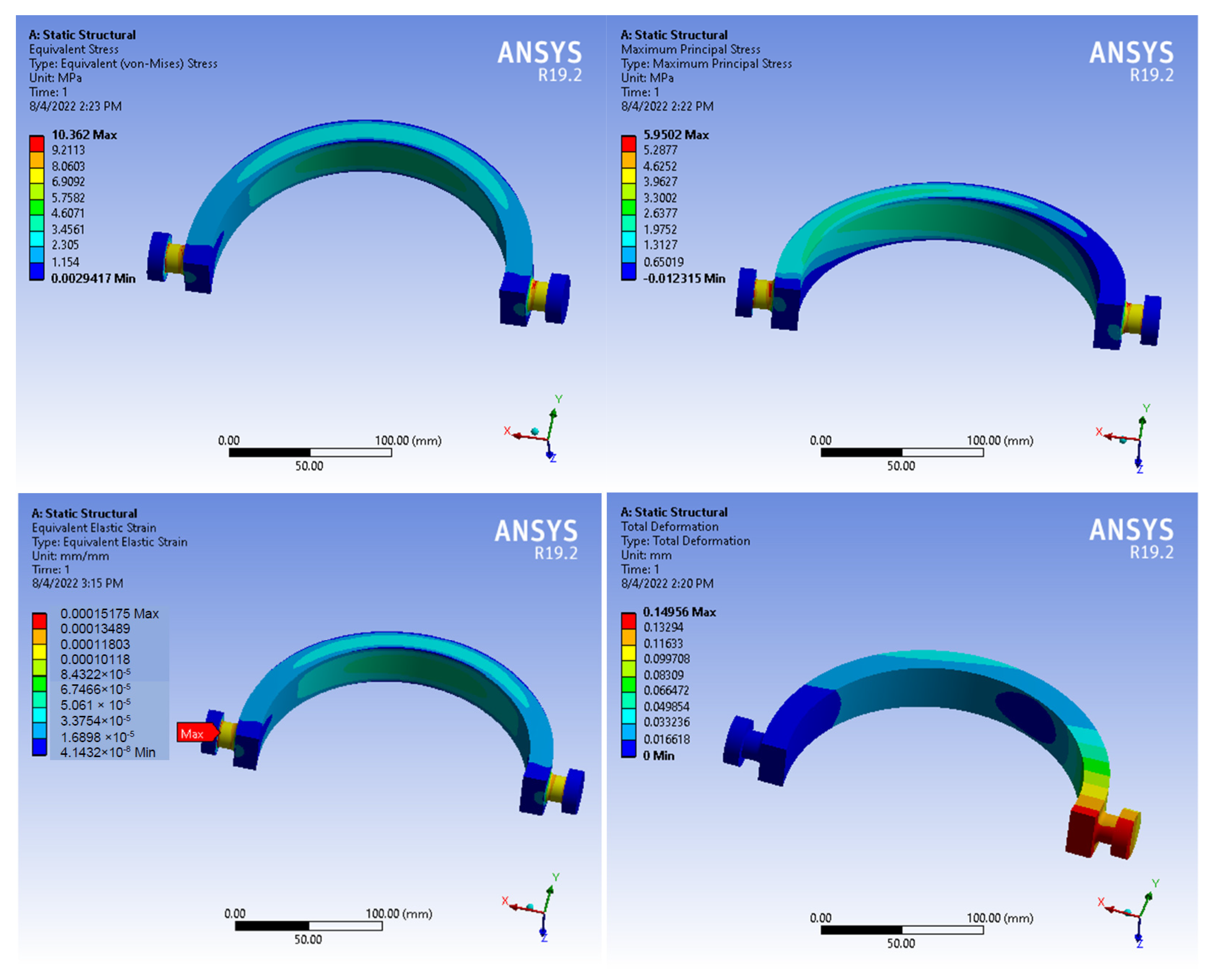
Figure 34.
Results of mechanical stresses, displacements, and strains for non-optimized structure.
Figure 34.
Results of mechanical stresses, displacements, and strains for non-optimized structure.
Figure 35.
Response chart for P6—Equivalent Stress Maximum vs. P1 and P3.
Figure 35.
Response chart for P6—Equivalent Stress Maximum vs. P1 and P3.
Figure 36.
Response chart for P4—Solid Mass vs. P1 and P3.
Figure 36.
Response chart for P4—Solid Mass vs. P1 and P3.
Figure 37.
Results of mechanical stresses, displacements, and deformations for the optimized structure.
Figure 37.
Results of mechanical stresses, displacements, and deformations for the optimized structure.
Figure 38.
The time history diagram for the flexion–extension motion of the ParReEx-wrist robotic system.
Figure 38.
The time history diagram for the flexion–extension motion of the ParReEx-wrist robotic system.
Figure 39.
The time history diagram for the radial–ulnar deviation motion of the ParReEx-wrist robotic system.
Figure 39.
The time history diagram for the radial–ulnar deviation motion of the ParReEx-wrist robotic system.
Figure 40.
Evolution of the RMS values for the connection forces in Couplings A and B.
Figure 40.
Evolution of the RMS values for the connection forces in Couplings A and B.
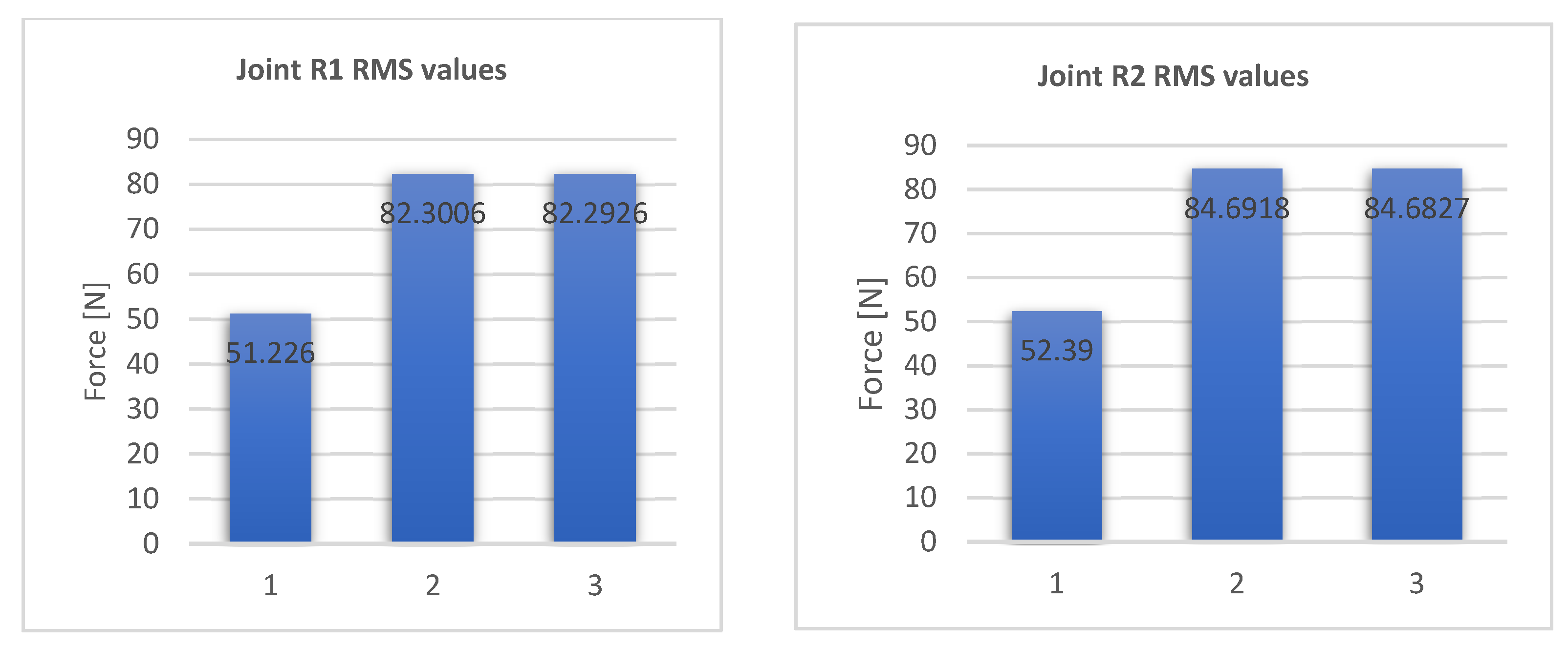
Figure 41.
Evolution of the RMS values for the connection forces in Joints R1 and R2.
Figure 41.
Evolution of the RMS values for the connection forces in Joints R1 and R2.
Figure 42.
Evolution of the maximum values for the moments of actuation for flexion–extension and radial–ulnar deviation motions.
Figure 42.
Evolution of the maximum values for the moments of actuation for flexion–extension and radial–ulnar deviation motions.
Table 1.
Bevel gear geometric parameters.
Table 1.
Bevel gear geometric parameters.
| | Value | Gear 1 | Gear 2 |
|---|
| Parameter | |
|---|
| No. of teeth | 39 | 39 |
| Orientation of rotation axis | 0, 90, 0 | 90, 90, 0 |
| Face width (mm) | 25.4 | 25.4 |
| Back cone distance (mm) | 10 | 15 |
| Pitch angle (°) | 19.747 | 70.253 |
| Pitch apex | 0 | 0 |
| Bore radius (mm) | 2 | 2 |
| Mean spiral angle (°) and direction | 35, LH | 35, RH |
| Outer trans. module (mm) | 4.535 | 4.535 |
| Tooth depth and width | Data Type I-ISO23509 |
| Profile shift coefficient | 0.505 | −0.505 |
| Dedendum factor | 1.25 | 1.25 |
| Thickness mod. coef. | 3.7 × 10⁻² | −5.5 × 10⁻² |
Table 2.
Bevel gear material properties.
Table 2.
Bevel gear material properties.
| |
Value | Gear1, Gear 2 |
|---|
|
Parameter | |
|---|
| Material type | Steel |
| Density (kg/m3) | 7801 |
| Young’s Modulus (N/m2) | 2.07 × 10¹¹ |
| Poisson ratio | 0.33 |
Table 3.
Bevel gear contact parameters.
Table 3.
Bevel gear contact parameters.
| Parameter | Value |
|---|
| Stiffness (N/mm2) | 5 × 10⁵ |
| Contact exponent | 1.1 |
| Damping coefficient | 5000 |
| Penetration (mm) | 0.01 |
| Static friction coefficient | 0.11 |
| Static friction transition velocity (mm/s) | 0.2 |
| Dynamic friction coefficient | 0.10 |
| Dynamic friction transition velocity (mm/s) | 0.5 |
Table 4.
Joint A connection force components.
Table 4.
Joint A connection force components.
| |
Component | Joint A Fx | Joint A Fy | Joint A Fz | Joint A MAG |
|---|
|
Parameter | |
|---|
| Min | 0.6315 | 60.8693 | −2.4821 | 64.3436 |
| Max | 20.8049 | 111.7138 | 88.6393 | 142.1042 |
| Avg | 11.8015 | 93.2991 | 37.1483 | 104.7257 |
| RMS | 13.9479 | 95.1698 | 49.6273 | 108.2345 |
Table 5.
Joint B connection force components.
Table 5.
Joint B connection force components.
| |
Component | Joint B Fx | Joint B Fy | Joint B Fz | Joint B MAG |
|---|
|
Parameter | |
|---|
| Min | 11.002 | 0.2556 | 19.9511 | 30.7333 |
| Max | 25.8542 | 0.3771 | 29.4384 | 32.6581 |
| Avg | 19.391 | 0.3084 | 24.0797 | 31.6122 |
| RMS | 20.1699 | 0.3118 | 24.3394 | 31.6122 |
Table 6.
Joint R1 connection force components.
Table 6.
Joint R1 connection force components.
| |
Component | Joint R1 Fx | Joint R1 Fy | Joint R1 Fz | Joint R1 MAG |
|---|
|
Parameter | |
|---|
| Min | −0.1407 | −51.1415 | −39.9417 | 35.325 |
| Max | 13.994 | −32.1514 | 4.533 | 63.5811 |
| Avg | 7.2739 | −44.6805 | −15.7091 | 50.263 |
| RMS | 8.9958 | 45.1932 | 22.3775 | 51.226 |
Table 7.
Joint R2 connection force components.
Table 7.
Joint R2 connection force components.
| |
Component | Joint R2 Fx | Joint R2 Fy | Joint R2 Fz | Joint R2 MAG |
|---|
|
Parameter | |
|---|
| Min | −14.4231 | 28.4593 | −17.9002 | 36.502 |
| Max | 6.4731 | 61.2824 | −19.281 | 64.5064 |
| Avg | −5.6765 | 48.3102 | −2.6405 | 21.6015 |
| RMS | 9.5789 | 49.7893 | 13.7125 | 52.39 |
Table 8.
Joint C connection force components.
Table 8.
Joint C connection force components.
| |
Component | Joint C Fx | Joint C Fy | Joint C Fz | Joint C MAG |
|---|
|
Parameter | |
|---|
| Min | −20.9865 | −144.671 | 15.4783 | 30.957 |
| Max | −0.0759 | −26.8092 | 85.5258 | 168.3648 |
| Avg | −8.4707 | −67.4532 | 38.9441 | 78.4077 |
| RMS | 11.2895 | 78.3566 | 45.2392 | 91.18 |
Table 9.
Joint friction parameters.
Table 9.
Joint friction parameters.
| Parameter | Value |
|---|
| Mu static | 0.2 |
| Mu dynamic | 0.15 |
| Friction arm (mm) | 10 |
| Bending friction arm (mm) | 10 |
| Pin radius (mm) | 5 |
| Stiction Transition velocity | 0.1 |
| Max. stiction deformation | 0.01 |
| Friction torque preload | 0 |
| Effect | Stiction only |
Table 10.
Robot motion parameters.
Table 10.
Robot motion parameters.
| |
Component | Motion 1 Torque (Nm) | Motion 2 Torque (Nm) |
|---|
|
Parameter | |
|---|
| Min | 0 | 0 |
| Max | 1.8086 | 5.5927 |
| Avg | 0.8143 | 4.3763 |
| RMS | 0.9317 | 4.4156 |
Table 11.
Joint A connection force components.
Table 11.
Joint A connection force components.
| |
Component | Joint A Fx | Joint A Fy | Joint A Fz | Joint A MAG |
|---|
|
Parameter | |
|---|
| Min | −3.7855 | 99.3604 | −32.0278 | 99.3604 |
| Max | 32.514 | 210.0206 | 129.7281 | 210.0206 |
| Avg | 15.0504 | 150.641 | 38.4032 | 150.641 |
| RMS | 19.5913 | 153.1624 | 65.5017 | 153.1624 |
Table 12.
Joint B connection force components.
Table 12.
Joint B connection force components.
| |
Component | Joint B Fx | Joint B Fy | Joint B Fz | Joint B MAG |
|---|
|
Parameter | |
|---|
| Min | 10.4354 | 0.1475 | 11.5174 | 11.5174 |
| Max | 39.1768 | 0.3846 | 30.0259 | 30.0259 |
| Avg | 24.8299 | 0.2639 | 20.6054 | 20.6054 |
| RMS | 26.8299 | 0.2767 | 21.6025 | 21.6025 |
Table 13.
Joint R1 connection force components.
Table 13.
Joint R1 connection force components.
| |
Component | Joint R1 Fx | Joint R1 Fy | Joint R1 Fz | Joint R1 MAG |
|---|
|
Parameter | |
|---|
| Min | −0.6321 | −94.2472 | −69.4304 | 58.9881 |
| Max | 26.2981 | −54.6674 | 8.8217 | 116.7565 |
| Avg | 11.9904 | −72.4773 | −23.7857 | 81.0712 |
| RMS | 15.3428 | 73.2824 | 34.1712 | 82.3006 |
Table 14.
Joint R2 connection force components.
Table 14.
Joint R2 connection force components.
| |
Component | Joint R2 Fx | Joint R2 Fy | Joint R2 Fz | Joint R2 MAG |
|---|
|
Parameter | |
|---|
| Min | −27.1507 | 44.5072 | −34.8471 | 57.757 |
| Max | 10.8219 | 115.4258 | 31.153 | 119.6574 |
| Avg | −9.6479 | 77.8998 | −5.9878 | 83.4607 |
| RMS | 16.3354 | 79.8368 | 23.0639 | 84.6918 |
Table 15.
Joint C connection force components.
Table 15.
Joint C connection force components.
| |
Component | Joint C Fx | Joint C Fy | Joint C Fz | Joint C MAG |
|---|
|
Parameter | |
|---|
| Min | −38.152 | −226.9065 | 18.9705 | 39.0085 |
| Max | −2.303 | −32.8579 | 131.0045 | 264.6976 |
| Avg | −18.3145 | −101.217 | 58.4376 | 118.4064 |
| RMS | 21.8939 | 114.4402 | 66.0721 | 133.9455 |
Table 16.
Circular guide modal parameters.
Table 16.
Circular guide modal parameters.
| Mode Number | Frequency (Hz) | Mode Number | Frequency (Hz) |
|---|
| 7 | 597.685 | 16 | 1.299 × 10⁴ |
| 8 | 1538.863 | 17 | 1.546 × 10⁴ |
| 9 | 1828.696 | 18 | 2.315 × 10⁴ |
| 10 | 2804.835 | 19 | 2.827 × 10⁴ |
| 11 | 3835.677 | 20 | 2.987 × 10⁴ |
| 12 | 4032.088 | 21 | 6.923 × 10⁴ |
| 13 | 5993.852 | 22 | 8.053 × 10⁴ |
| 14 | 6743.001 | 23 | 1.343 × 10⁵ |
| 15 | 9246.1609 | 24 | 1.808 × 10⁵ |
Table 17.
Robot motion parameters in Case 3.
Table 17.
Robot motion parameters in Case 3.
| |
Component | Motion 1 Torque | Motion 2 Torque |
|---|
|
Parameter | |
|---|
| Min | 0.0013 | 2.431 |
| Max | 1.8086 | 5.5339 |
| Avg | 0.8143 | 4.3712 |
| RMS | 0.9316 | 4.4062 |
Table 18.
Joint A connection force components.
Table 18.
Joint A connection force components.
| |
Component | Joint A Fx | Joint A Fy | Joint A Fz | Joint A MAG |
|---|
|
Parameter | |
|---|
| Min | −2.2236 | 99.6565 | −42.8897 | 115.1857 |
| Max | 62.8521 | 210.1286 | 98.7351 | 231.5797 |
| Avg | 30.9324 | 150.7614 | 17.3479 | 163.231 |
| RMS | 38.4147 | 153.2828 | 48.9964 | 165.4441 |
Table 19.
Joint B connection force components.
Table 19.
Joint B connection force components.
| |
Component | Joint B Fx | Joint B Fy | Joint B Fz | Joint B MAG |
|---|
|
Parameter | |
|---|
| Min | 0.4806 | −0.8625 | −1.6387 | 0.4815 |
| Max | 9.1875 | 0.4868 | 1.0018 | 9.2307 |
| Avg | 8.8505 | 0.4033 | −0.4287 | 8.91 |
| RMS | 8.853 | 0.4095 | 0.9483 | 8.9131 |
Table 20.
Joint R1 connection force components.
Table 20.
Joint R1 connection force components.
| |
Component | Joint R1 Fx | Joint R1 Fy | Joint R1 Fz | Joint R1 MAG |
|---|
|
Parameter | |
|---|
| Min | −0.6319 | −94.247 | −69.4296 | 59.116 |
| Max | 26.2983 | −54.7853 | 8.8217 | 116.7565 |
| Avg | 11.2983 | −72.4702 | −23.7732 | 81.0625 |
| RMS | 15.3456 | 73.4702 | 34.1647 | 82.2926 |
Table 21.
Joint R2 connection force components.
Table 21.
Joint R2 connection force components.
| |
Component | Joint R2 Fx | Joint R2 Fy | Joint R2 Fz | Joint R2 MAG |
|---|
|
Parameter | |
|---|
| Min | −27.1509 | 44.6085 | −34.8469 | 57.8858 |
| Max | 10.8215 | 115.425 | 31.1528 | 119.6571 |
| Avg | −9.6539 | 77.8865 | −5.9965 | 83.4504 |
| RMS | 16.3394 | 79.8258 | 23.066 | 84.6827 |
Table 22.
Joint C connection force components.
Table 22.
Joint C connection force components.
| |
Component | Joint C Fx | Joint C Fy | Joint C Fz | Joint C MAG |
|---|
|
Parameter | |
|---|
| Min | −38.152 | −226.9063 | 19.031 | 39.1179 |
| Max | −2.3031 | −32.9627 | 131.0044 | 264.6962 |
| Avg | −18.3109 | −101.1899 | 58.422 | 118.375 |
| RMS | 21.8903 | 114.4194 | 66.0601 | 133.9213 |
Table 23.
Displacement of the center of mass of the circular guide.
Table 23.
Displacement of the center of mass of the circular guide.
| |
Component | Depl Tx (m) | Depl Ty(m) | Depl Tz(m) | Depl T Mag(m) |
|---|
|
Parameter | |
|---|
| Min | −0.031 | −0.0018 | 0.0865 | 0.0866 |
| Max | −0.0042 | 7.620 × 10⁻⁶ | 0.0865 | 0.0919 |
| Avg | −0.0176 | −9.243 × 10⁻⁴ | 0.0865 | 0.0887 |
| RMS | 0.0199 | 0.0011 | 0.0865 | 0.0887 |
Table 24.
Deformation of the center of mass of the circular guide.
Table 24.
Deformation of the center of mass of the circular guide.
| |
Component | Def Dx(m) | Def Dy(m) | Def Dz(m) | Def D Mag(m) |
|---|
|
Parameter | |
|---|
| Min | −6.638 × 10⁻⁸ | −4.132 × 10⁻⁸ | −6.603 × 10⁻⁸ | 2.46 × 10⁻¹¹ |
| Max | −1.948 × 10⁻¹¹ | 1.405 × 10⁻¹¹ | −3.737 × 10⁻¹² | 9.960 × 10⁻⁸ |
| Avg | −6.256 × 10⁻⁸ | −2.094 × 10⁻⁸ | −5.735 × 10⁻⁸ | 8.83 × 10⁻⁸ |
| RMS | 6.268 × 10⁻⁸ | 2.412 × 10⁻⁸ | 5.739 × 10⁻⁸ | 8.834 × 10⁻⁸ |
Table 25.
Design points of design-of-experiments.
Table 25.
Design points of design-of-experiments.
| |
Param. | Design Point | P1—FBlend4.FD1 (mm) | P2—FBlend3.FD1 (mm) | P3—XYPlane.R1 (mm) | P4—Solid Mass (kg) | P5—Equivalent Stress Maximum (MPa) |
|---|
|
No. | |
|---|
| 1 | 1 DP | 3 | 3 | 92 | 0.54397 | 10.362 |
| 2 | 2 | 2.7 | 3 | 92 | 0.54391 | 10.159 |
| 3 | 3 | 3.3 | 3 | 92 | 0.54403 | 10.3 |
| 4 | 4 | 3 | 2.7 | 92 | 0.54391 | 10.125 |
| 5 | 5 | 3 | 3.3 | 92 | 0.54403 | 10.304 |
| 6 | 6 | 3 | 3 | 82.8 | 0.79132 | 10.205 |
| 7 | 7 | 3 | 3 | 101.2 | 0.27269 | 19.837 |
| 8 | 8 | 2.7561 | 2.7561 | 84.52 | 0.7468 | 10.415 |
| 9 | 9 | 3.2439 | 2.7561 | 84.52 | 0.7469 | 10.297 |
| 10 | 10 | 2.7561 | 3.2439 | 84.52 | 0.7469 | 10.302 |
| 11 | 11 | 3.2439 | 3.2439 | 84.52 | 0.74699 | 10.364 |
| 12 | 12 | 2.7551 | 2.7561 | 99.48 | 0.32514 | 13.127 |
| 13 | 13 | 3.2439 | 2.7561 | 99.48 | 0.32523 | 13.126 |
| 14 | 14 | 2.7561 | 3.2439 | 99.48 | 0.32523 | 13.131 |
| 15 | 15 | 3.2439 | 3.2439 | 99.48 | 0.32533 | 13.127 |
Table 26.
Min–Max Search.
Table 26.
Min–Max Search.
| Name | P1—FBlend4.FD1 (mm) | P2—FBlend3.FD1 (mm) | P3—XYPlane.R1 (mm) | P4—Solid Mass (kg) | P5—Equivalent Stress Maximum (MPa) |
|---|
| Output Parameter Minimums |
| P4-Solid Mass | 2.7 | 2.7 | 101.2 | 0.27258 | 19.837 |
| P5—Equivalent Stress Maximum | 3.033 | 3.2561 | 89.656 | 0.60933 | 10.211 |
| Output Parameter Maximums |
| P4—Solid Mass | 3.3 | 3.3 | 82.8 | 0.79144 | 10.351 |
| P5—Equivalent Stress Maximum | 3.183 | 2.7264 | 101.2 | 0.27268 | 19.837 |
Table 27.
Response surface parameters.
Table 28.
Optimization study.
Table 29.
Optimization candidate points.


 ,
, 


 1
1 1.954
1.954 2.7089