Prediction of the Equivalent Steering Angle of a Front-Wheel, High-Clearance Paddy Field Management Machine

Abstract

To solve the problem of poor steering consistency for each steering wheel of a four-wheel, independent-steering, high-clearance paddy field management machine, given that the true steering angle of the front wheel cannot be directly obtained through the left and right front wheels steering angle value, a BP (Back Propagation) neural network equivalent steering angle prediction method based on signal feature extraction is proposed in this paper, which can be used to obtain the equivalent steering angle of the front wheel. First, the kinematics model of the paddy field management machine was constructed with the prediction of the steering angle of the management machine as the object. The body was set up in two application environments of cement ground and paddy field, two moving speeds (25 cm/s, 50 cm/s) and three preset steering angles (0°, ±10°) to form six motion modes. The steering angle of the front wheel of the body, the three-axis acceleration of the body, and the angular velocity of the z-axis under twelve conditions were collected. Combining the collected data with the actual trajectory data of the differential BeiDou, the feasibility analysis of the equivalent steering angle prediction was carried out. With the aim of determining an appropriate combination of input factors for optimal equivalent steering angle prediction by the BP neural network, we used FFT (Fast Fourier Transform) and power spectrum conversion to extract and analyze the signal features of the airframe attitude data and obtain the frequency characteristics of the peak power point of the power spectrum, respectively. Through a factor combination test, the optimal BP neural network training factors were determined and, finally, we confirmed that the rotation angles of the front wheels and the z-axis angular velocity may be used as effective training factors. In our investigation on the test set, the mean square error of the equivalent steering angle was found to be less than 0.66°, demonstrating that our approach is effective for obtaining the true steering angle of the front wheel.

1. Introduction

With the development of digital agriculture, the working environment for agricultural practitioners has been improved and their labor intensity has been reduced [1]. As a key technology in precision agriculture, automatic driving has been greatly emphasized by an increasing number of researchers [2,3,4,5,6]. Unmanned agricultural machinery can play a role in reducing labor intensity, decreasing input costs, and increasing profitability [7]. High-precision navigation and driving systems can reduce damage to crops by repeated-trajectory driving [8], while high-precision steering angle detection benefits the navigation performance of autonomous driving systems [9,10].

Precise detection of the steering angle of autonomous agricultural machinery can be achieved by direct or indirect means [11]. Cucchiara et al. [12] established a steering wheel motion model and realized the steering wheel angle measurement by detecting and tracking the main features on the steering wheel. Paul et al. [13] proposed a wireless steering wheel angle sensor using optical media for angle detection and gave a wireless steering wheel angle sensor. The modeling and simulation results of steering sensor and wired steering system were presented, and the feasibility of the system was discussed based on the simulation results. Yang et al. [14] mounted a CCD sensor on the vehicle to form a visual detection system, extracted the contour edge points of the steering wheel image collected by the CCD, and performed ellipse fitting on the edge points to detect the steering angle. Nagasaka et al. [15] directly obtained the steering angle data of rice harvesters using an absolute value rotary encoder, while Hu et al. [16] utilized a displacement sensor and four-link angle sensor to calculate a tractor’s front wheel angle, which was achieved by adopting the least squares fitting method to calibrate the sensor, in order to establish a sensor model for identification of the tractor’s steering angle. Santana-Fernandez et al. [17] carried out gyroscope-based steering angle detection research, in which they established an autoregressive–moving-average (ARMA) model of the microelectromechanical system (MEMS) drift signal and integrated a Kalman filter. Miao et al. [18] proposed a wheel steering angle measurement system based on dual global navigation satellite system (GNSS) antennas and dual MEMSs, combined with an adaptive Kalman filter designed with respect to the drift and accumulated error of the gyroscope. In an agricultural machinery navigation test, the average error of the straight-line driving angle was 0.06° and the variance of the error was 0.215°. Zhang et al. [19] studied the calibration and detection of the steering wheel angle of wheeled tractors, taking a Levo M904-D wheeled tractor as the research platform and adopting a WYH-3-type contactless angle sensor.

In this study, four-wheel independent-steering paddy field machinery (shown in Figure 1) was taken as the object of steering angle detection research. The four-wheel independent-steering paddy field management machine was multi-functional and was developed for deep mud paddy field management. Each of the four wheels can be turned independently and the chassis ground clearance and wheelbase heights can be adjusted. The management machine adopts the combination of four hydraulic motors and a reducer to drive four-wheel independently and adopts a combination of four hydraulic motors and a reducer to perform four-wheel independent steering, through the use of computer control, special driving modes (e.g., horizontal driving, in situ steering, and small turning radii) may be realized to meet the needs of small-area field operations in hilly and mountainous areas. Given that the rear wheels only perform steering control in specific scenarios such as small-radius transitions or lateral shifts, this study only focused on the detection of the steering angle of the front wheels during travel. Due to a gear drive gap in the steering mechanism, the actual steering may have a free rotation angle of around 2°. At the same time, there are control differences in independent steering, which make it difficult to accurately synchronize the steering or determine the steering state. The existence of the four-wheel steering swimming angle gap makes it difficult to build a rigorous mathematical model based on the four-wheel steering angle value to obtain the real steering angle. With the help of the self-learning, self-organization, and the adaptive characteristics of the neural network algorithm, it can fully approximate any complex. The advantage of the nonlinear relationship can make up for the uncertain influence of the swimming steering angle on the detection of the true steering angle of the airframe. In this study, the BP neural network algorithm was used to predict the steering angle of the front wheel to obtain the effective steering angle of the front wheel.

2. Materials and Methods

2.1. Hardware and Software

Since the research focused on the steering of the front wheel, the rear wheel was mechanically fixed by mechanical self-locking to eliminate the influence of the free shaking of the rear wheel on the front steering detection. Steering angle detection for the front wheels was carried out using a magnetic sensitive angle sensor (GT-B). Attitude data for the whole machine were collected with the vehicle unit as the core (Figure 2).

An STM32F103RC was adopted as the core processor of the onboard unit, and real-time, high-speed data exchange was achieved with an electronic control unit (ECU) through the CAN interface, in order to obtain real-time data from the steering angle sensor of the ECU unit. A remote controller was used for remote operation of the chassis, a data acquisition board performed serial port expansion to collect the nine-axis attitude data of the body, and the data were analyzed using software on a PC.

The attitude sensor included Witer’s intelligent WT901C nine-axis attitude sensor module. The acceleration accuracy of the sensor was 0.01 m/s² and the angular velocity accuracy was 0.05°/s. The differential BeiDou positioning system of UniStrong was used to calibrate the movement trajectory of the center position of the rear axle of the chassis. The base station model was BNBASE-010C, the mobile station model was E2020C5, and the positioning data update rate was 10 Hz, and data analysis was based on the MATLAB 2019A(Commercial mathematical software produced by MathWorks, USA) environment.

2.2. Acquisition and Evaluation of Effective Input Factors for a BP Neural Network Based on Sensor Feature Extraction

During the working process of the steering wheel, there are high-frequency disturbances and spikes in the steering angle data. If all of the signal input sources are used as input for BP neural network prediction, the training complexity will inevitably increase. At the same time, the input factors of the BP neural network not only affect the output, but also the operational efficiency of the system. The MIV algorithm is typically used to analyze the correlation between each input factor and the output. However, MIV is related to the number of iterations and other variables, meaning that there is generally some uncertainty. In this study, by extracting the sensor characteristic parameters, and by analyzing the signal characteristics, the parameters with consistent spectra could be selected as effective factor input criteria. Through comparative experiments, the validity of the above principles was verified, effective input factors were obtained, and actual data were tested to evaluate the validity of the prediction.

2.2.1. Sensor Signal Analysis and Feature Extraction

We use the spectrum analysis method, whereby we used the sensor signals as input for spectrum feature extraction, in order to obtain the common features of sensor parameters.

First, we performed an FFT (Fast Fourier Transform) on the data to obtain the power spectrum and determine the corresponding peak value. The frequency value corresponding to the peak area was used as a feature reference for low-pass filtering and data analysis, in order to eliminate high-frequency system interference.

Classical frequency spectrum estimation methods, such as the indirect method, Bartlett method, and Welch method, usually include a periodic graph. In this study, the common periodogram method was applied for power spectrum conversion.

The periodogram method regards the N-point observation data $x\left(n\right)$ of the random signal observation data $x_N\left(n\right)$ as a signal with limited energy. We used the Fourier transform of $x_N\left(n\right)$ to obtain $x_N\left(e^{j\omega }\right)$, then took the amplitude squared and divided it by N to estimate the true power spectrum $P\left(e^{j\omega }\right)$ of $x\left(n\right)$. ${\widehat{P}}_{per}\left(e^{j\omega }\right)$ represents the power spectrum estimated by the periodogram method, calculated as:

$${\widehat{P}}_{per}\left(e^{j\omega }\right)=\frac{1}{N}|X_N\left(\omega \right){|}^2.$$

(1)

As the FFT is used for spectrum transformation, it can be calculated as follows:

$${\widehat{P}}_{per}\left(k\right)=\frac{1}{N}|X_N\left(k\right){|}^2.$$

(2)

In this way, power spectrum conversion of the input information can be completed.

According to summarization and analysis of the common characteristics of the sensor signal spectrum, effective training data could be gathered by selecting an appropriate input combination of training factors; that is, one that combines the characteristic elements.

2.2.2. Analysis of the Equivalent Steering Angle Model of the Front Wheels

Given the low driving speed of the four-wheel independent-steering paddy field machinery, the steering angle of the rear wheels remains at 0° under normal walking conditions, while the front wheels are used for steering. Thus, the classic bicycle kinematics model can be used to analyze the machinery’s steering trajectory. Figure 3 depicts the case where this model is adapted to the paddy field management machine.

In Figure 3, θ is the deflection direction of the chassis relative to the coordinate system, L is the wheelbase of the chassis, δ is the steering angle of the steering wheel, and R is the current turning radius. Due to the inconsistency between the input parameter unit and size range of the wheel angle, to facilitate neural network training, normalization processing is required, as follows:

$$x=\frac{x-\overline{x}}{\sigma },$$

(3)

where $\overline{x}$ is the average of the corresponding input data, while $\sigma$ is the standard deviation of the input data.

The equivalent wheel angle is calibrated using the BeiDou differential positioning system:

$$v_{x,i}=\frac{x_i-x_{i-1}}{t},v_{y,i}=\frac{y_i-y_{i-1}}{t},$$

(4)

where $v_{x,i}$ and $v_{y,i}$ represent the velocities in x and y directions at time i, respectively.

At the same time, the corresponding accelerations $a_{x,i}$ and $a_{y,i}$ can be obtained using the velocity:

$$a_{x,i}=\frac{v_{x,i}-v_{x,i-1}}{t},a_{y,i}=\frac{v_{y,i}-v_{y,i-1}}{t}.$$

(5)

Based on this, the calculation formula for the curvature is as follows:

$$k_i=\left|\frac{v_{x,i}{a}_{y,i}-a_{x,i}{v}_{yi}}{{\left(v_{x,i}{}^2+v_{y,i}{}^2\right)}^{3/2}}\right|.$$

(6)

The turning radius of the vehicle can be obtained as follows:

$$R=\frac{1}{k}.$$

(7)

The equivalent front wheel steering angle is as follows:

$$\delta =\arctan (\frac{L}{R}).$$

(8)

2.2.3. Equivalent Steering Angle Prediction Based on a BP Data Network

A BP neural network can provide non-linear mapping which approximates a given mapping function from input to output. When considering the equivalent steering angle and steering angle sensor, it is difficult to establish a direct logical relationship for the independent steering state of the front wheels; however, equivalent steering angle prediction using a BP neural network is feasible.

Therefore, in this study, a BP neural network was used to achieve equivalent steering angle prediction, where gradient search technology was adopted in the learning process of the network to correct the weights through back-propagation of the errors, in order to minimize the difference between the actual and expected output of the network. Figure 4 shows a BP network model with a hidden layer, where ${\delta }_i$ are the input units (which can be one of many characteristic parameters, such as the wheel wobble amplitude, frequency, speed, or body attitude), $V_j$ are the hidden layer units (which are related to the weights ${\omega }_{ij}$ obtained from network training), and ${\mathcal{Q}}_1$ is the output (which is the equivalent steering angle of the front wheel of the machinery).

Considering inputs $\delta$, the input to a hidden layer unit $V_i$ can be expressed as:

$$r_j={{\displaystyle \sum }}_{k=1}^m{w}_{jk}{\delta }_k,$$

(9)

The output of hidden layer unit $V_i$ is:

$$V_j=f\left(r_j\right),$$

(10)

where the function $f$ is the activation function, for which non-linear terms are typically introduced to improve the expression ability of the neural network. In this study, we used the Sigmoid activation function.

The input to the output unit is:

$$H_1={\displaystyle \sum }_{q=1}^j{W}_{1q}{V}_q={\displaystyle \sum }_{q=1}^j{W}_{1q}f\left({\displaystyle \sum }_{k=1}^m{w}_{jk}{\delta }_k\right),$$

(11)

Finally, the output unit also needs to be non-linearized using an activation function, namely,

$${\mathcal{Q}}_1=g\left(H_1\right),$$

(12)

For any input or output unit, the loss function can be used as the index to learn the weights of the hidden layer of the neural network; that is, a new weight can be selected by adding an appropriate $\Delta \omega$ to the original weight $\omega$. The gradient descent method can be used to reduce the loss function as much as possible as the number of iterations increases, such that the local minimum value can be ascertained.

For the connection weight between an input unit and a hidden layer unit, the chain rule can be used to obtain:

$$\Delta {\omega }_{ij}=-\eta \frac{\partial E}{\partial {\omega }_{ij}}=-\eta \frac{\partial E}{\partial V_i}\frac{\partial V_i}{\partial {\omega }_{ij}}=\eta {\xi }_i{\delta }_j,$$

(13)

$$\mathrm{where}{\xi }_i=f\left(h_i\right){{\displaystyle \sum }}_i{W}_{ij}{\xi }_i$$

(14)

and $\eta$ is the learning step, which is set according to experience. Similarly, the weight between a hidden layer unit and the output unit can be obtained as follows:

$$\Delta W_{jk}=-\eta \frac{\partial E}{\partial W_{jk}}=\eta {\xi }_j{V}_k,$$

(15)

$${\xi }_j=g\left(h_j\right)\left({\delta }_j-{\mathcal{Q}}_j\right).$$

(16)

According to the above, the neural network weight matrix can be obtained using the gradient descent method, based on the input and output layer data:

$$w_{new}=w_{old}+\Delta w^{\prime },$$

(17)

$$\Delta w^{\prime }=\left\{\Delta w,\Delta W\right\}.$$

(18)

2.2.4. Loss Function Selection and Training Effect Evaluation

The mean squared error (MSE) loss function (shown in Formula (19)) was used to evaluate the training effect:

$$los{s}_2=\frac{1}{N{{\displaystyle \sum }}_{i=1}^N{\left(y_{gt}-\widehat{y}\right)}^2},$$

(19)

where $y_{gt}$ is the equivalent wheel angle and $\widehat{y}$ is the wheel angle estimated by the neural network.

Eighty percent of all data collected were used as the training set for neural network training and learning. After training, the remaining 20% of data were used as a test set, in order to evaluate the training effect.

3. Results and Discussion

3.1. Experimental Conditions and Simulation Analysis

The experimental data acquisition met the following standards:

(a)

The test adopted the front wheel steering control method, and we set the control steering angles (steering sensor detection) to 0°, −10°, and +10°.

(b)

For data collection, the serial port of the airborne ECU unit was used to directly output the front wheel steering angle, driving speed $v$, and body attitude parameters, where the driving speed $v$ was taken as the average of the speeds of the two rear wheels. The body attitude parameters included the machinery’s three-axis angular velocity $({\omega }_x$, ${\omega }_y$, ${\omega }_z)$, the three-axis acceleration $(a_x$, $a_y$, $a_z)$, and the geomagnetic relative heading angle.

(c)

A differential BeiDou positioning system was used to detect and calibrate the driving track, speed, and heading angle. Through coordinate conversion, absolute x and y coordinates and a course angle ${\delta }^{\prime }$ based on the position of the starting point were obtained. The velocity data were converted by coordinate values to obtain the calibration velocity, and trajectory curve information was obtained using Formula (6).

(d)

Taking the starting point and the end point of the test trajectory data as the reference, combined with the sampling time, the Formula (8) was applied to obtain the actual steering angle value.

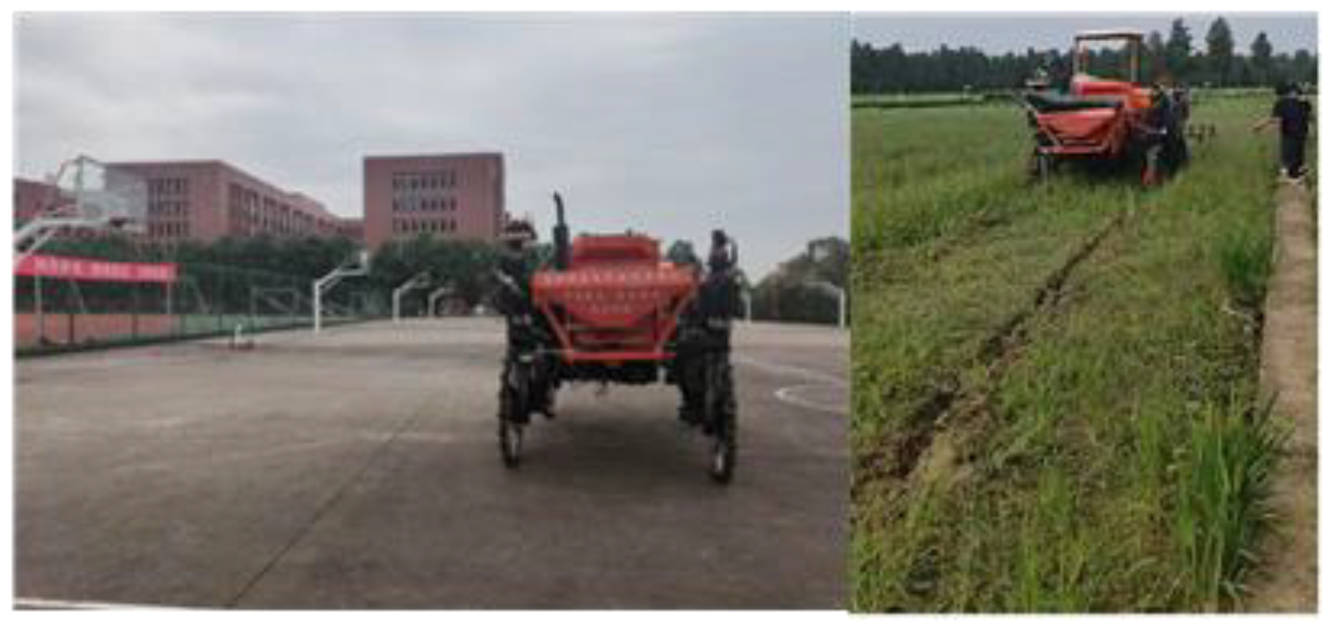
To simulate the actual running conditions of the paddy field management machine, two test environments—cement ground and a subsiding paddy field—were selected (see Figure 5).

3.2. Feasibility and Necessity of Equivalent Steering Angle Prediction

In the experiment, in two environments of cement ground and paddy field, the paddy field management machine collected the test data at two traveling speeds of 25 cm/s and 50 cm/s, and the steering control angle was divided into three cases: 0°, −10°, and +10°. According to the collected data, the least squares circle fitting method was used to fit and analyze the driving trajectory in the environment of matlab2019a to verify the feasibility and effectiveness of the equivalent steering angle prediction. A fitted track for cement ground is shown in Figure 6. The red part in the figure is the actual driving displacement of the paddy field management machine, while the gray part is the trajectory fitting circle. Modes 1, 3, and 5 are 0°, −10° and +10° steering angles at a speed of 25 cm/s. Likewise, modes 2, 4, and 6 were performed at a speed of 50 cm/s.

When analyzing Figure 6, it can be seen that when the steering angle of the stable steering wheel is changed, the trajectory can be fitted to a closed circle, and the steering 3angle of the front wheel obtained after fitting deviated from the steering angle of the set control. When this is 0°, the corresponding deviations of steering angles were −0.5° and 0.1°; for the corresponding deviation of −10°, the steering angles were −2.5° and −0.3°; and, when the corresponding deviation is 10°, the steering angles were −0.2° and 0.9°. The subsiding paddy field’s (mode 1 to 6) driving data fitting circles are shown in Figure 7.

From Figure 7, it can be seen that when the steering angle of the stable steering wheel changed, the trajectory line could be fitted to a closed circle, and the front wheel steering angle obtained after fitting deviated from the steering angle set control. For 0°, the corresponding deviations of steering angles were 1.2° and 1.7°; at the corresponding deviation of −10°, the steering angles were 0.3° and −0.3°; and, with the corresponding deviation of 10°, the steering angles were 3° and 8.1°. Based on the overall analysis of Figure 6 and Figure 7, combined with our analysis of the raw data, the following conclusions can be drawn:

• In terms of the asymmetric oscillations between the left and right steering wheels, the frequency and amplitude of the steering oscillations conformed to a normal distribution and could form a fitting circle, which proves the feasibility of the equivalent steering angle prediction.
• When affected by ground resistance, there was a certain control deviation from the preset steering angle control of the hydraulic steering motor. The effectiveness of the left and right steering wheel controls differed, resulting in a difference between the target control angles of the left and right steering wheels, indicating that prediction of the equivalent steering angle of the machinery is necessary.

3.3. Spectral Characteristics Analysis of the Sensor Data

Through analysis of the raw data of the left and right front wheels on the cement ground, after performing FFT transformation, power spectrum transformation, and low-pass filtering, the analysis data graphs shown in Figure 8 and Figure 9 were obtained.

It can be seen from Figure 8 and Figure 9, that there were large fluctuations in the steering angles of the left and right front wheels (close to 2°). This deviation is similar to the free rotation angle of the front wheels, which is mainly related to the vibration of the machinery, the movement of structural parts, and the vibration due to an uneven ground.

When we performed FFT and power spectrum transformation, the maximum power points corresponding to the oscillation frequencies of the left and right steering wheels were found to be around 0.2 Hz. As such, the characteristic value was extracted, and the frequency data were filtered.

Next, we analyzed the remaining 11 modes for the cement ground and subsiding paddy field. The obtained analysis data are provided in

Table 1. Power spectrum frequencies for cement ground parameters.

	Mode	One	Two	Three	Four	Five	Six
Index
Left front wheel steering angle		0.2	0.21	0.24	0.22	0.22	0.21
Right front wheel steering angle		0.21	0.22	0.19	0.19	0.21	0.18
x-axis acceleration		0	0	0	0	0	0
y-axis acceleration		0	0	0	0	0	0
z-axis acceleration		0	0	0	0	0	0
x-axis angle speed		None	None	None	None	None	None
y-axis angle speed		None	None	None	None	None	None
z-axis angle speed		0.9	1.53	1.14	1.52	1.51	1.44
Heading angle		0	0	0	0	0	0

and

Table 2. Power spectrum frequencies for subsiding paddy field parameters.

	Mode	One	Two	Three	Four	Five	Six
Index
Left front wheel steering angle		0.25	0.23	0.27	0.17	0.23	0.27
Right front wheel steering angle		0.27	0.20	0.23	0.21	0.20	0.23
x-axis acceleration		0	0	0	0	0	0
y-axis acceleration		0	0	0	0	0	0
z-axis acceleration		0	0	0	0	0	0
x-axis angle speed		None	None	None	None	None	None
y-axis angle speed		None	None	None	None	None	None
z-axis angle speed		1.50	1.55	1.52	0.39	1.24	0.98
Heading angle		0	0	0	0	0	0

.

By analyzing the data in Table 1 and Table 2, the peak frequency points of the power spectra of the left and right front wheels were found to be maintained at about 0.2 Hz under different speeds, ground environments, and steering angles. The z-axis angular velocity appeared under different environments; however, there were certain peak frequency points in the power spectrum, while the power spectra of the x and y axial angular velocity data presented no characteristic peak power frequency points. The peak frequency of the acceleration data power spectrum was generally close to 0 Hz and the fluctuation range was small, reflecting the nature of the machinery’s inherent vibration. Similarly, the power spectrum frequency of the attitude sensor heading angle data was also close to 0 Hz.

Characteristic differences in the attitude signal were determined through spectral analysis, indicating whether there was a peak frequency point in the power spectrum. Based on this, the BP neural network equivalent steering angle prediction input factors were further extracted and verified.

3.4. BP Data Network Input Factor Selection and Training

The front wheel steering angle detection value was found to be directly related to the equivalent steering angle. Therefore, the left and right front wheel steering angle data were selected as basic input factors, and the corresponding spectral peak frequency was used as the basis for time dimension selection for the benchmark training subset. Therefore, a 5 s time period was used for the training subset. The filtered data were processed using various time periods, in order to obtain 148 training subsets. We randomly selected 80% of the subset as the training set, while the remaining 20% were used as the test set for evaluating the training effect.

The presence or absence of a power spectrum peak frequency point in the attitude data was taken as an input factor. We evaluated the effectiveness by performing training followed by evaluation with three combinations, in order to confirm the effectiveness of feature extraction. The combinations used are described in

Table 3. Training input factor combinations.

Combination No.	Mix of Factors
1	Left and right rotation angles, z-axis angular velocity
2	Left and right rotation angles, x- and y-axis acceleration, z-axis angular velocity
3	Left and right rotation angles, x- and y-axis acceleration

.

The network structure of the corresponding BP neural network is shown in Figure 10.

The training process (in terms of the training loss) is depicted in Figure 11.

A total of 500 epochs were used for training the neural network. The loss decreased throughout the training process, indicating that the network converged well.

Once the test sets with the three training input combinations had been implemented, a comparison table between the test and real values could be compiled, as shown in

Table 4. Training factor test results for the three combinations.

Combination 1		Combination 2		Combination 3
True Value	Expected Value	True Value	Expected Value	True Value	Expected Value
−0.33	−0.64	−0.33	−0.28	−0.54	−0.63
−0.54	−0.13	−0.15	−0.09	−0.33	3.96
0.21	0.25	−0.33	−0.02	1.21	−1.50
0.21	0.41	−2.51	−2.14	1.21	0.30
0.94	1.48	−0.54	−0.30	0.10	1.26
3.07	2.72	−0.54	−0.39	0.94	−0.03
0.94	1.51	3.07	1.50	0.94	−0.58
1.21	1.18	−0.33	−0.20	0.94	0.52
1.21	1.21	3.07	3.17	8.10	1.82
−0.15	0.25	8.10	5.48	0.10	−0.09
1.70	0.27	0.10	0.16	0.21	−2.92
1.21	1.54	0.21	0.02	3.07	1.75
8.10	9.60	1.21	1.78	0.10	1.27
3.07	3.54	−0.15	−0.33	0.21	0.21
1.70	1.34	−0.54	−0.31	1.21	1.11
0.10	0.65	−0.54	−0.17	0.21	0.97
0.10	0.52	−0.33	0.04	−2.51	−2.00
−0.15	0.14	−0.54	−0.33	0.21	0.60
−2.51	−2.77	8.10	7.57	−0.15	−0.76
0.21	0.23	−0.33	−0.26	0.21	−1.62
−2.51	−2.69	3.07	2.85	1.21	4.09
1.70	0.95	0.21	0.29	−0.33	0.27
1.21	0.78	8.10	8.05	1.21	0.79
−0.54	−0.19	−2.51	−2.07	3.07	1.08
−2.51	−3.08	3.07	2.97	3.07	1.23
−0.33	−0.63	3.07	1.36	−0.54	−0.90
1.21	−0.38	1.70	0.25	0.10	0.62
−0.15	0.35	−0.15	−0.09	3.07	1.32
−0.15	1.51	0.21	0.04	−0.33	1.33
−0.33	−0.27	1.21	1.39	−0.15	0.24

.

The corresponding mean squared errors (MSEs) are given in

Table 5. Test set MSEs for different input combinations.

	Combination 1	Combination 2	Combination 3
MSE	0.44	0.54	3.7

.

By training with the three combinations of input factors and conducting verification on the corresponding test sets, we found that when the left and right front wheel steering angle parameters with the peak frequency points of the power spectrum and the z-axis rotation angular velocity parameter were used as the BP neural network training input factors to obtain the best prediction effect, the corresponding mean square error was 0.44 and the mean square error of the equivalent steering angle was less than 0.66°, indicating a good prediction effect. For the other combinations, although the number of training input factors was increased, the prediction effect decreased. Therefore, by using a BP neural network equivalent steering angle prediction algorithm with the characteristics of the peak frequency point of the power spectrum, we could effectively predict the equivalent steering angle of the front wheels of an independent-steering paddy field management machine.

4. Conclusions

In this work, an effective steering angle prediction method was proposed for front-wheel independent-steering paddy field machinery. By collecting data on the steering angle and body attitude sensors, then adopting FFT and power spectrum conversion to extract the spectrum characteristics of the sensors, we determined that the peak frequency of the steering angle sensor power spectrum was 0.2 Hz, and that the z-axis angle speed power spectrum presented a peak frequency, while systemic characteristic information of the power spectrum frequency could not be found with the other sensors. On this basis, different combinations were selected as input factors for equivalent steering angle prediction using the proposed BP neural network, in order to verify the validity of the input factors consisting of characteristic information on the peak frequency points of the power spectra. Finally, the left and right front wheel steering angle values and z-axis steering angle speed were selected as the optimal input factors for equivalent steering angle prediction, and the training set was divided using basic rules for data processing with a data analysis frequency of 0.2 Hz. By analyzing and processing 148 sample data points obtained under two different ground states, two different driving speeds, and three preset steering angles, the predicted mean squared error on the test set was found to be 0.44, the equivalent steering angle mean squared error was less than 0.66°, and the equivalent steering angle prediction was good, which essentially meets the accuracy requirements for the navigation control steering angle.

Compared with the steering angle value obtained by directly calculating the steering angle of the left and right steering wheels, the steering angle was calculated by Formula (20):

$$\mathsf{\gamma }=({\mathsf{\alpha }}_{\mathrm{Left}}+{\mathsf{\alpha }}_{\mathrm{Right}})/2$$

(20)

By comparing the steering angle value of the body obtained by using the above calculation formula with the real steering angle value, it was found that the mean square error of steering angle detection was 1.97, and the maximum steering angle deviation was 4.81°. Compared with the traditional method, the neural network was used to calculate the equivalent steering angle. The mean square value of prediction error was increased by 1.53, and the maximum error angle was 1.66°, which could obtain better detection effect and meet the accuracy requirements of navigation control steering angle.

Compared with the conventional BP neural network training, which uses massive data input to improve the training effect, this study extracted the signal features of the left and right front wheel steering angles, x, y, z-axis acceleration values, and z-axis angular velocity values to obtain effective training input factors. In the comparison test, compared with using more input factors, only using three input factors of left and right front wheel steering angle value and z-axis rotation angular velocity, the equivalent steering angle prediction effect was better, which provides a new method for the selection of BP neural network training factors. The study also provides the possibility for the fast and effective implementation of the BP neural network algorithm.

Since the sample time for neural network training is 5 s, for applications that require continuous steering adjustment, such as non-linear assisted navigation and driving, auxiliary means such as multi-sensor fusion are needed to improve the real-time detection. These are points to be aware of when steering the system for unmanned navigation.

References

- Li, M.; Kenji, I.; Liu, Z.; Wu, W.; Li, J.; Wu, B. Positioning algorithm for agricultural machinery omnidirectional vision positioning system. Trans. Chin. Soc. Agric. Eng. 2013, 29, 52–59. [Google Scholar]
- Li, D.; Li, Z. System analysis and development prospect of unmanned farming. Trans. Chin. Soc. Agric. Mach. 2020, 51, 1–12. [Google Scholar]
- Boryga, M.; Kołodziej, P.; Gołacki, K. Application of Polynomial Transition Curves for Trajectory Planning on the Headlands. Agriculture 2020, 10, 144. [Google Scholar] [CrossRef]
- Sportelli, M.; Luglio, S.M.; Caturegli, L.; Pirchio, M.; Magni, S.; Volterrani, M.; Frasconi, C.; Raffaelli, M.; Peruzzi, A.; Gagliardi, L.; et al. Trampling Analysis of Autonomous Mowers: Implications on Garden Designs. AgriEngineering 2022, 4, 592–605. [Google Scholar] [CrossRef]
- Julio-Rodríguez, J.d.C.; Rojas-Ruiz, C.A.; Santana-Díaz, A.; Bustamante-Bello, M.R.; Ramirez-Mendoza, R.A. Environment Classification Using Machine Learning Methods for Eco-Driving Strategies in Intelligent Vehicles. Appl. Sci. 2022, 12, 5578. [Google Scholar] [CrossRef]
- Baek, E.-T.; Im, D.-Y. ROS-Based Unmanned Mobile Robot Platform for Agriculture. Appl. Sci. 2022, 12, 4335. [Google Scholar] [CrossRef]
- Han, S.; He, Y.; Fang, H. Recent development in automatic guidance and autonomous vehicle for agriculture: A review. J. Zhejiang Univ. 2018, 44, 381–391. [Google Scholar]
- Roviramás, F. Sensor architecture and task classification for agricultural vehicles and environments. Sensors 2010, 10, 11226–11247. [Google Scholar] [CrossRef] [Green Version]
- Dickon, M.; Goguchi, N.; Zhang, Q.; Reid, J.; Will, J. Sensor-Fusion Navigator for Autometed Guidance of Off-Road Vehicles. U.S. Patent 6445983 B1, 3 September 2002. [Google Scholar]
- Geng, A.; Hu, X.; Liu, J.; Mei, Z.; Zhang, Z.; Yu, W. Development and Testing of Automatic Row Alignment System for Corn Harvesters. Appl. Sci. 2022, 12, 6221. [Google Scholar] [CrossRef]
- Han, X.; Kim, H.; Kim, J.; Yi, S.; Moon, H.; Kim, J.; Kim, Y. Path-tracking simulation and field tests for an auto-guidance tillage tractor for a paddy field. Comput. Electron. Agric. 2015, 112, 161–171. [Google Scholar] [CrossRef]
- Cucchiara, R.; Prati, A.; Vigetti, F. Steering wheel’s angle tracking from camera-car. In Proceedings of the IEEE IV2003 Intelligent Vehicles Symposium, Columbus, OH, USA, 9–11 June 2003; pp. 406–409. [Google Scholar]
- Paul, D.; Kim, T.H. On the feasibility of the optical steering wheel sensor: Modeling and control. Int. J. Autom. Technol. 2011, 12, 661–669. [Google Scholar] [CrossRef]
- Yang, J.; Shi, Z.; Shu, T. An Image-Based Method to Detect Steering Angle of Moving Vehicle. J. Xi’an Jiaotong Univ. 2013, 47, 76–78. [Google Scholar]
- Nagasaka, Y.; Umeda, N.; Kanetai, Y.; Taniwaki, K.; Sasaki, Y. Autonomous guidance for rice transplanting using global positioning and gyroscopes. Comput. Electron. Agric. 2004, 43, 223–234. [Google Scholar] [CrossRef]
- Hu, S.; Shang, Y.; Liu, H. Comparative test between displacement and four-bar indirect measurement methods for tractor guide wheel angle. Trans. CSAE 2017, 33, 76–82. [Google Scholar]
- Santana-Fernández, J.; Gomez-Gil, J.; Del-Pozo-San-Cirilo, L. Design and implementation of a GPS guidance system for agricultural tractors using augmented reality technology. Sensors 2010, 10, 10435–10447. [Google Scholar] [CrossRef] [PubMed] [Green Version]
- Miao, C.; Chu, H.; Cao, J.; Sun, Z.; Yi, R. Steering angle adaptive estimation system based on GNSS and MEMS gyro. Comput. Electron. Agric. 2018, 153, 196–201. [Google Scholar] [CrossRef]
- Zhang, Z.; Wang, G.; Luo, X.; He, J.; Wang, J.; Wang, H. Detection method of steering wheel angle for tractor automatic driving. J. Agric. Mach. 2019, 50, 352–357. [Google Scholar]