Split-Spectrum Processing with Raised Cosine Filters of Constant Frequency-to-Bandwidth Ratio for L(0,2) Ultrasonic Guided Wave Testing in a Pipeline

Abstract

Ultrasonic guided wave (UGW) nondestructive testing suffers from poor signal interpretation accuracy caused by the coherent noise that is related to dispersion, multi-mode and mode conversion. In order to split the L(0,2) UGW from the coherent noise, split-spectrum processing with raised cosine filters of constant frequency-to-bandwidth ratio (FBR-RC-SSP) is proposed. With the advantages of time domain resolution and frequency domain split, FBR-RC-SSP is studied based on time-frequency analysis using the chirplet transform, and the effects of filter parameters on signal-to-noise ratio gain (SNRG) and defect-to-coherent noise gain (DCRG) are explained. The excellent effects of eliminating the coherent noise and improving the signal resolution in FBR-RC-SSP are reported by the validation of synthesized, simulated and experimental UGW signals, of which the average SNRG and DCRG are 22.92% and 23.71% higher than those of traditional SSP using Gaussian filters, and it has the potential to locate and characterize defects in further UGW testing research.

1. Introduction

Ultrasonic guided wave (UGW) testing is a promising nondestructive testing method that affords low attenuation, high propagation velocity and high accuracy, and it can be utilised for high-efficiency, non-contact, long-distance and large-scale detection of a pipeline [1,2]. There are two inherent characteristics of dispersion and multi-mode in UGW, which are manifested in the fact that UGW velocity varies with the frequency and the geometry of the waveguide, and multiple modes of UGWs exist at a given frequency [3]. When a UGW propagates in a waveguide, it travels in various modes: longitudinal L(0,m), torsional T(0,m) and flexural F(n,m), where n and m denote circumferential order and module [4]. The ideal axisymmetric modes L(0,2) and T(0,1) in their non-dispersive regions are preferred in UGW testing for reducing the interpretation complexity of the detection signal, where L(0,2) UGWs with high propagation velocity are more sensitive to circumferential defects compared with those of the T(0,1) UGW [5].

The pure UGW with desired mode is difficult to be excited singly, where UGWs with undesired modes can also be excited for the imperfect experimental conditions and multi-mode characteristics, and the mode conversion may be caused when the UGW with the desired mode encounters asymmetric defects, of which flexural UGWs may arise [6]. The wave packets of UGWs with desired, undesired and flexural modes may be overlapped for the difference in the propagation velocity, indicating that signal energy spreads out over time and space domain, and it is not conducive to UGW testing interpretation on account of the low signal resolution [7,8]. Pedram et al. [7] refer to UGWs other than the desired mode as coherent noise.

There are some studies using pulse compression (PuC), which increases the excitation energy while modulating the signal, to improve the signal resolution, and the received signal is extracted by cross-correlation with an excitation signal [9]. Mahal et al. [10] studied the modulation effects of Chiript, Barker and Golay codes with a small main lobe width and found that the SNRs (Signal to Noise Ratios) after modulation by the above three methods were significantly higher than those using a Hanning window sinusoidal signal. Fan et al. [11] proposed a hybrid coding excitation method using the convolution of the Barker and Golay code, and the results showed a significant improvement in SNR and peak sidelobe levels to approximately 32 dB and approximately −24 dB, respectively. However, PuC requires the design of excitation waveform, the performance of optimal excitation sequence depends on the detection conditions and the elimination of coherent noise is limited [12].

Dispersion compensation (DC) is another signal processing method commonly applied in UGW testing, where the coherent noise can be eliminated by reversing the effect of dispersion and multi-mode on the desired mode UGW in the time/space domain [13]. Downs et al. [14] obtained UGW signals through an original 64-element phased array, extracted wavenumber and spectrum analysis coherent noise, used Auld’s electromechanical reciprocity relationship and variational method to extract mode contributions and finally used a dispersion compensation method to eliminate the coherent noise. On the basis of DC, Luo et al. [15] proposed two wideband Lamb wave time-frequency dispersion analysis methods: time-frequency compensation transform and time-frequency de-dispersion transform, and the results show that both methods can obtain high-resolution Lamb wave signals. However, DC requires a priori knowledge of dispersion and propagation distance, which is often difficult to know in the UGW testing of long-distance pipelines and unknown pipeline structures [16].

Split spectrum processing (SSP) can split the UGWs with multi-mode by separating the received signal into a sub-signal group in the frequency domain and recombining them in the time domain without the knowledge of dispersion and propagation distance [17,18]. SSP was developed from the frequency-agile techniques in the radar field and then applied to conventional ultrasonic inspection to reduce the effect of coarse-grain scattering and improve the SNR [19], which is rarely applied in UGW testing. Only a few studies focus on the SNR enhancement of the T(0,1) UGW signal using SSP. Pedram et al. [7,20] studied the parameters of an SSP filter suitable for T(0,1) UGW signals and compared the effects of different signal recombination methods through synthetic and experimental signals, and the results showed that SSP does have the ability to enhance the signal interpretation accuracy. However, to the best of the authors’ knowledge, there is no study on the L(0,2) UGW signal processed by SSP. In addition, Pedram et al. only considered the dispersion as the cause of coherent noise where multi-mode should also be concluded, and they just applied SSP to UGW testing without any improvement.

In order to improve the signal interpretation accuracy of UGW testing, SSP with raised cosine filters of constant frequency-to-bandwidth ratio (FBR-RC-SSP) was proposed by the filter bank design (Section 2). Based on the time-frequency analysis using the chirplet transform, the characteristics of dispersion and multi-mode of synthesized signal composed of L(0,1), L(0,2), F(n,1) and F(n,3) UGW were studied (Section 3). The effects of filter parameters on signal-to-noise ratio gain (SNRG) and defect-to-coherent noise ratio gain (DCRG) were explained (Section 4). Section 5 and Section 6 evaluated the processing effect of FBR-RC-SSP on the simulated and experimental UGW signals with multi-defect, and Section 7 concluded the paper finally.

2. Split Spectrum Processing

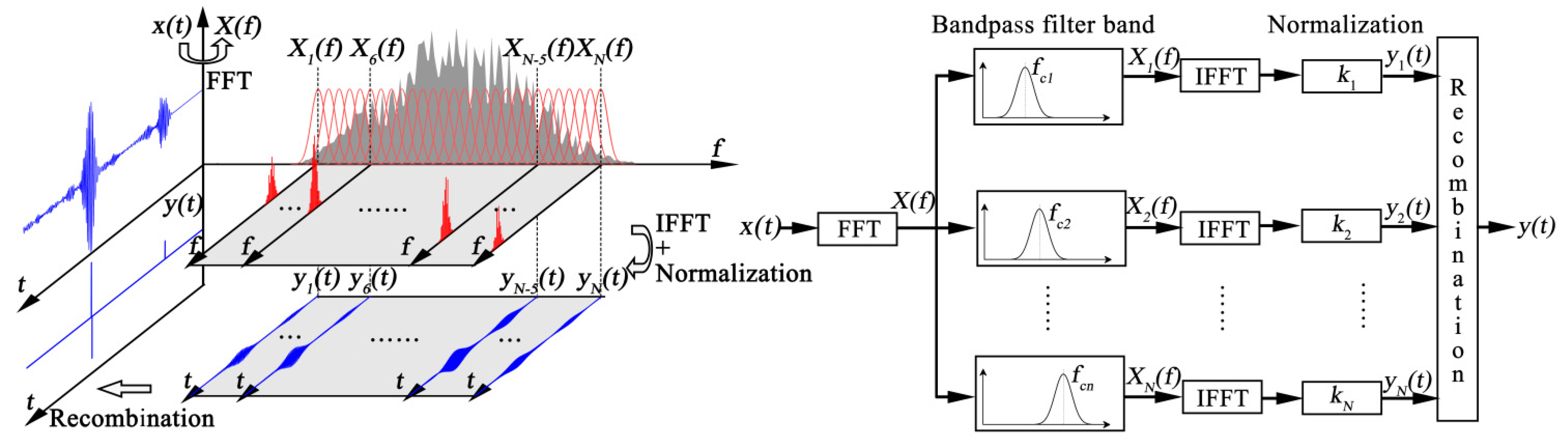
The schematic diagram of split spectrum processing (SSP) is illustrated in Figure 1. First, the fast Fourier transform (FFT) is used to transform an input signal x(t) in time domain into a frequency–domain signal X(f), which is split into a sub-band signal group X_i(f) (I = 1,2,…,N, N denotes the number of filters) in the frequency domain by an intersecting bandpass filter bank (increasing center frequency). Then, the inverse FFT (IFFT) is employed on X_i(f) and normalization to obtain a time–domain sub-band signal group y_i(t). Finally, nonlinear signal recombination methods are utilized to produce an output signal y(t). The function principle behind SSP is the frequency sensitivity among the UGWs with desired and other modes; that is, a different X_i(f) contains the desired UGW mode with similar amplitude and the modes of other UGWs with different amplitudes.

Gaussian bandpass filters are commonly used in SSP due to the ease of implementation [21]. On the one hand, the cross-correlation coefficient of coherent noise components in adjacent X_i(f) should be controlled to be as small as possible for better coherent noise elimination, indicating that the overlapping region of adjacent filters is required to be as small as possible. On the other hand, the non-overlapping filter bank should be able to avoid the “picket fence” effect, wherein substantial information will be lost, which is not conducive to the signal interpretation [22]. Hence, the filter bank design should take into account the above requirements.

2.1. Filter Bank Design

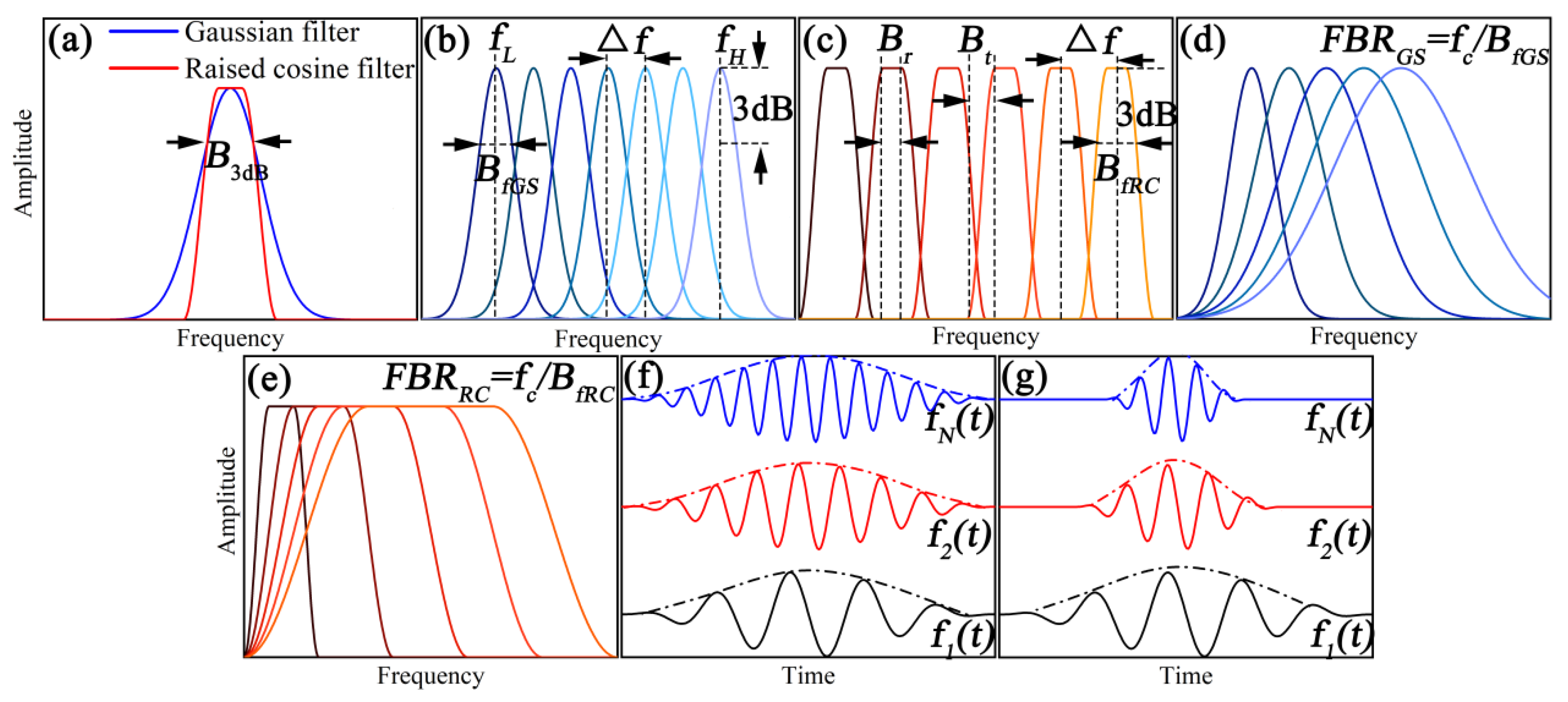
Unlike the Gaussian (GS) filters, the raised cosine (RC) filters, which are shown in Figure 2a, have transition bands in the shape of a truncated, raised cosine cycle, and the energy contained in the RC filter is mostly concentrated around the center frequency for the flat top design [23]. It is easy to foresee that the RC filters can show a better split effect compared with that of GS filters, considering the degree of overlap in RC filters is lower than the GS filters, given the constant filter spacing. According to the frequency distributions of GS and RC filters in Figure 2b,c, the filter parameters shared by GS and RC filters are total processing bandwidth B (B = f_H − f_L, where f_H and f_L are the high and low cutoff frequencies, respectively). Filter bandwidth B_fGS or B_fRC and filter spacing Δf and B_fRC can be further replaced by the transition bandwidth B_t and the flat top width B_r.

The frequency impulse of RC filter with center frequency f_ci is given by:

$$R{C}_i(f)=\{\begin{array}{ll}1/2\left\{1+\cos \left[\pi (f-f_{ci}+B_r/2)/B_t\right]\right\}& f_{ci}-B_r/2-B_t\le f\le f_{ci}-B_r/2\\ 1& f_{ci}-B_r/2\le f\le f_{ci}+B_r/2\\ 1/2\left\{1+\cos \left[\pi (f-f_{ci}-B_r/2)/B_t\right]\right\}& f_{ci}+B_r/2\le f\le f_{ci}+B_r/2+B_t\\ 0& otherwise\end{array}$$

(1)

To the end of achieving a better split, the relatively small filter bandwidth B_f is recommended compared with total processing bandwidth B, but the time resolution would be poor to some extent. It is beneficial to apply the filters with variable bandwidth, so the GS and RC filters with constant frequency-to-bandwidth (FBR) ratio are proposed, as shown in Figure 2d–g. It can be observed that the time impulse of the FBR-RC filter becomes narrower, whereas B_f becomes wider as f_c increases compared with those of the RC filter, indicating the improvement of time resolution.

2.2. Signal Recombination Methods

The signal recombination methods considered in this paper are based on order statistics and phase observation, which conclude Normalized Minimization (NORM-MIN), Mean (MEAN), Frequency Multiplication (FM), Polarity Thresholding (PT), Polarity Thresholding with Minimization (PTM) and Scaled polarity threshold (SPT), and they are expressed as described in [24]:

$$y_{NORM-MIN}(t)=\min \left(\left|y_i\left(t\right)/{\max }_i\left(y_i\left(t\right)\right)\right|\right)$$

(2)

The output signal of NORM-MIN is the normalized minimum value of all sub-band signals y_i(t) (i = 1,2,…,N) at time t, which is suitable for the case where the defect signal amplitude is significantly higher than the coherent noise level; otherwise, the defect signal would not be completely preserved.

$$y_{MEAN}\left(t\right)={\displaystyle \sum _{i=1}^N{y}_i\left(t\right)}/N$$

(3)

MEAN retains the average value of all sub-band signals at each time t; it can reduce the coherent noise level by averaging, as the noise value varies in different sub-band signals. However, it is similar to NORM-MIN, which would get a great result when the coherent noise level is much lower than defect signal amplitude. Therefore, NORM-MIN and MEAN would not suitable for the high dispersive signals.

$$y_{FM}\left(t\right)={\displaystyle \prod _{i=1}^N{y}_i\left(t\right)}$$

(4)

The sub-band signals are multiplied by each other to generate the FM output signal, and this method could enhance the defect with large amplitude and reduce the noise level with low amplitude, which implies that FM has a good processing effect on low dispersive signals.

$$\begin{array}{l}{y}_{PT}\left(t\right)=\{\begin{array}{ll}x\left(t\right)& if y_i\left(t\right)<0 or \text{>}0, \forall i\\ 0& otherwise\end{array}\end{array}$$

(5)

The output signal of PT is the unprocessed signal x(t) at time t if all the sub-band signals are negative or positive; otherwise, it is zero. Thus, PT can eliminate the coherent noise, which is highly sensitive to the frequency and has a different sign in different sub-band signals. Although the requirements of PT are not as strict as those of the above methods, the defect signal amplitude should not be lower than the noise level.

$$\begin{array}{l}{y}_{PTM}\left(t\right)=\{\begin{array}{ll}\min y_i\left(t\right)& if y_i\left(t\right)<0 or \text{>}0, \forall i\\ 0& otherwise\end{array}\end{array}$$

(6)

$$\begin{array}{l}{y}_{SPT}\left(t\right)=\{\begin{array}{ll}\left|\frac{N_{+}-N_{-}}{N}\right|\min y_i\left(t\right)& if y_i\left(t\right)<0 or \text{>}0, \forall i\\ 0& othwewise\end{array}\end{array}$$

(7)

Both PTM and SPT are the combination of the minimization and PT, and the difference between them and PT is that the minimization of all sub-band signals at time t is retained when all the sub-band signals are negative or positive. N+ and N− are the total positive and negative numbers of the sub-band signal group. However, PTM and SPT may reduce the defect signal amplitude while reducing the noise level, which would influence the further quantitative analysis of defects.

3. Synthesized UGW Signal Analysis

3.1. UGW Characteristic Analysis

A low-carbon steel pipe with an outer diameter of 48 mm, a wall thickness of 5 mm and a length of 5.5 m was used, of which the dispersion curves of axisymmetric UGWs were drawn by PC_disp package [25] in Figure 3a,b. Since the UGW velocity is a function of frequency, the center frequency of UGW with the desired mode should be selected within the frequency band with little change in velocity. When the frequency is between 100 kHz and 150 kHz, it is easy to distinguish the L(0,2) UGW with a large and smooth phase and group velocities from other UGWs. The excitation frequency of the L(0,2) UGW was chosen as 110 kHz in this paper, and the corresponding phase and group velocity were 5460.86 m/s and 5350.47 m/s, respectively.

It is almost impossible to not excite T(0,m) (m ≥ 1) and L(0,m) (m ≥ 3) UGWs when L(0,2) is the desired mode and excitation frequency is 110 kHz, because the excitation conditions of the torsional UGW are quite different from those of the longitudinal UGW, and the cutoff frequencies of L(0,m) (m ≥ 3) UGWs are greater than 110 kHz. Therefore, the undesired L(0,1) UGW is most likely to appear with the excitation of the L(0,2) UGW. The excitation signal spectrum and the dispersion curves of the corresponding L(0,1) and L(0,2) asymmetric flexural UGWs are shown in Figure 3c,d. It can be seen that the phase velocity increases and group velocity decreases as the order n increases from 0 to 4, and velocity difference among L(0,2) and F(n,3) (1 ≤ n ≤ 4) UGWs is greater than that among L(0,1) and F(n,1) (1 ≤ n ≤ 4) UGWs in the excitation frequency band.

The normalized displacement distributions of the above UGWs were plotted in Figure 4. It can be concluded that the L(0,1) and F(n,1) UGWs are dominated by radial displacement and share similar distribution as n varies, whereas axial displacements with relatively large difference as n varies are dominant in the L(0,2) and F(n,3) UGWs. In addition, the dominant displacements decrease while circumferential displacements increase as n increases. The above phenomenon may be the cause of the velocity difference among UGWs, and the resolution of the L(0,2) UGW may be inevitably affected by other UGWs for the difference in displacement distributions and velocities.

3.2. UGW Signal Time-Frequency Analysis

The chirplet transform, a generalization of both the wavelet and the short-time Fourier transform, can extract signal components with specific instantaneous frequencies and group delays and overcome the shortcomings of conventional time-frequency representation solutions such as the short-time Fourier transform and the Wigner–Ville distribution, which may not achieve good UGW mode separation results, whereas multiple modes usually occupy the same frequency band and intersect each other in time. The standard definition of the chirplet transform is given by the inner product of a basis function g(t) and the signal x(t) [26]:

$$CT=\langle x(t),g(t)\rangle ={\displaystyle {\int }_{-\infty }^{\infty }x(t)}{g}^{*}(t)dt$$

(8)

$$g(t)=T_{t0}{F}_{w0}{S}_s{Q}_q{P}_{p}c(t)$$

(9)

where * denotes the complex conjugate, and g(t) and G(ω) are basis function and the Fourier transform of basis function. T_t0, F_ω0, S_s, Q_q, and P_p are the time shift, frequency shift, scaling, frequency shear and time shear operators, and the details are shown in

Table 1. Operations for the chirplet transform operators.

Operation		Transformation
Time shift Tt0	$T_{t0}c(t)=c(t-t_0)$	$t=t-t_0$	$w=w$
Frequency shift Fω0	$F_{w0}c(t)=c(t)\exp (i{w}_{0}t)$	$t=t$	$w=w-w_0$
Scaling Ss	$S_{S}c(t)=c(t/s)/\sqrt{s}$	$t=t/s$	$w=sw$
Frequency shear Qq	$Q_{q}c(t)=c(t)\exp (iq/2t^2)$	$t=t$	$w=w-qt$
Time shear Pp	$P_{p}c(t)=c(t)\exp (i{t}^2/2p)/\sqrt{ip}$	$t=t-pw$	$w=w$

. c(t) is one of the chirp signal families.

The basis function can be adjusted by the operators of shifting, scaling, and shearing, leading to the generation of five-dimensional space, which combines the projections of the short-time Fourier transform (time and frequency shift) and a wavelet transform (time shift and scaling).

The L(0,1), F(n,1), L(0,2) and F(n,3) (1 ≤ n ≤ 4) UGW synthesized signals propagating 0.8 m in time and frequency domains were plotted in Figure 5, of which the spectrums were plotted by the chirplet transform. Although the cutoff frequencies of F(3,3) and F(4,3) are 138.474 kHz and 180.279 kHz, which are larger than the center frequency of 110 kHz, their excitation is still possible, since their cutoff frequencies are in the excitation frequency band. Therefore, the frequencies of synthesized F(3,3) and F(4,3) are set as their cutoff frequencies. It can be observed that the wave packets of UGWs become wider while the propagation times become later with higher order n, which may be attributed to the increase in phase velocity and decrease in group velocity. In addition, it can also be found that the time/frequency resolution of the synthesized signal composed with L(0,1) and F(n,1) is poorer than that of the L(0,2) and F(n,3) synthesized signal.

Synthesized L(0,1), L(0,2), F(n,1) and F(n,3) UGW signals propagating 0.8 m in the time-frequency domain are shown in Figure 6a. It can be found that it would be difficult to distinguish L(0,2) from others only by the time domain signal, and the frequency domain signal may be easier to distinguish, but the spectrum obtained by the chirplet transform is based on a priori knowledge of dispersion and propagation distance. Figure 6b shows the synthesized signals at different propagation distances. It can be observed that the UGW signal with too large of a propagation distance or too long of a propagation time should be avoided on account of the wide wave packet and weak wave energy.

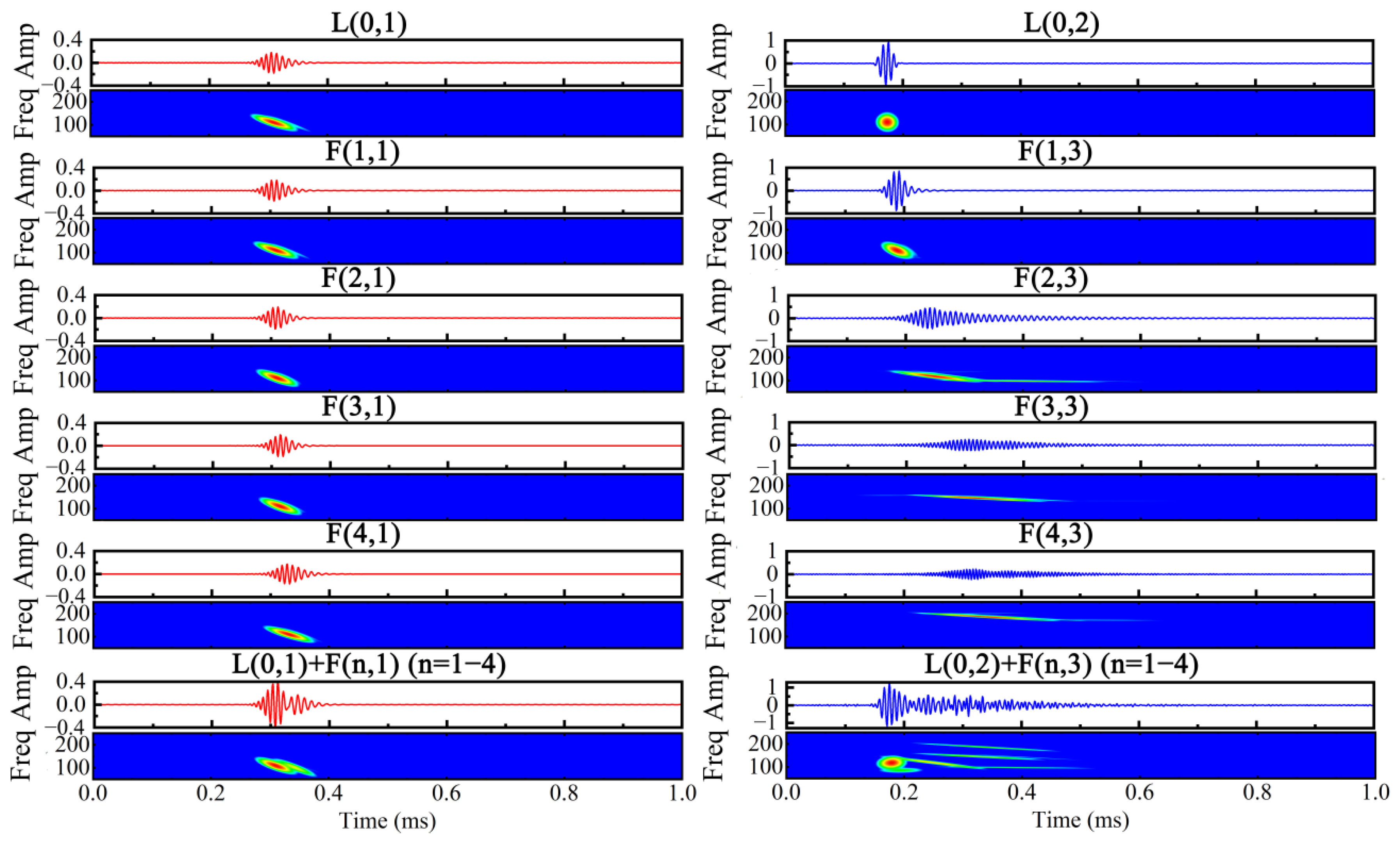
4. Filter Parameters Analysis

In order to be consistent with the real UGW testing signal, it is necessary to multiply the amplitude of the L(0,1) + F(n,1) + L(0,2) + F(n,3) synthesized signal with the propagation distance of 0.8 m by 0.6 as a defect echo, and the L(0,1) + F(n,1) + L(0,2) + F(n,3) synthesized signal with the propagation distance of 1.8 m is regarded as an end-reflected echo, as illustrated in Figure 7. Likewise, the resolution of the L(0,2) UGW will still be poor in the time-frequency domain because of the influence of other UGWs, and it is necessary to eliminate the coherent noise.

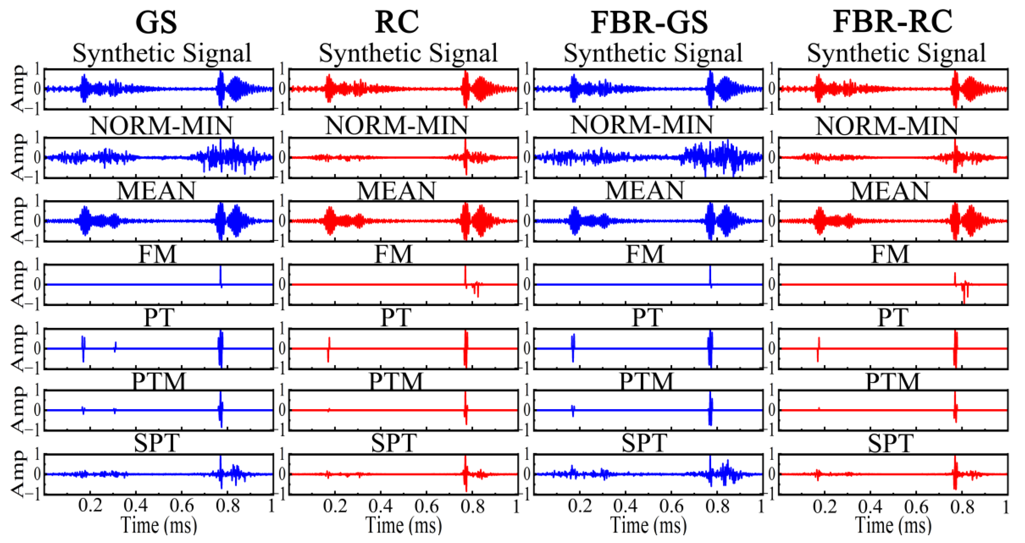
The SSPs based on GS, RC, FBR-GS and FBR-RC filters (B = B_3dB, B_fGS = B_fRC = B_3dB/10, ∆f = B_3dB/40, where B_3dB is the 3 dB bandwidth of unprocessed signal) are used to process the synthesized UGW signal, and the results are shown in Figure 8. It can be found that the interpretation accuracy improvement of NORM-MIN and MEAN are not significant, of which the coherent noise is not completely eliminated. Although FM can effectively improve SNR, it also eliminates the defect echo, which is inadvisable. PT, PTM and SPT show excellent processing effects, where the defect echoes are retained and coherent noise is eliminated. In addition, it can also be observed that FBR-SSPs are better than SSPs, which is consistent with the discussion in Section 2.1.

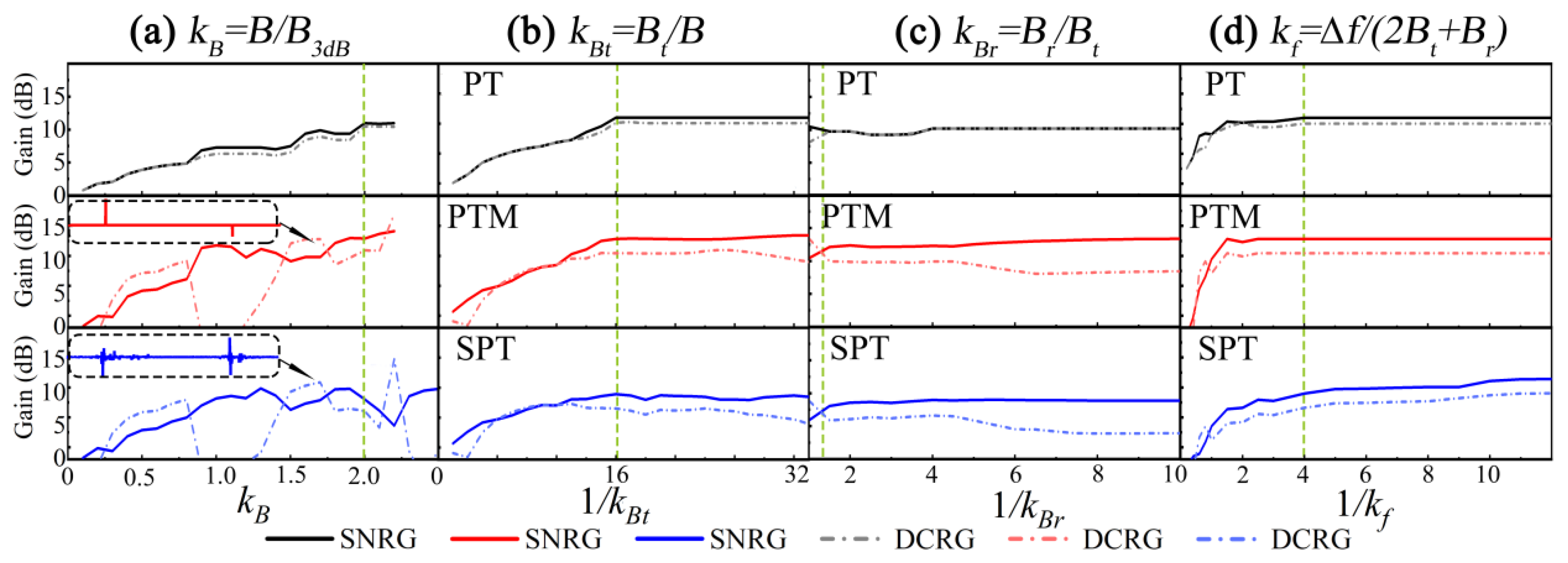
In order to achieve the best processing effect, it is necessary to choose the appropriate filter parameters for the parameter sensitivity of the SSP. The signal-to-noise ratio gain SNRG and defect-to-coherent noise gain DCRG are introduced to quantitatively measure the effects of parameters, of which the calculation formulas are as follows:

$$SNRG=20\left[{\log }_{10}\left(S_{out}/N_{out}\right)-{\log }_{10}\left(S_{in}/N_{in}\right)\right]$$

(10)

$$DCRG=20\left[{\log }_{10}\left(D_{out}/N_{out}\right)-{\log }_{10}\left(D_{in}/N_{in}\right)\right]$$

(11)

where S is the maximum amplitude of the signal, D is the amplitude of the defect echo, N is the coherent noise level calculated by the root mean square of the whole signal, and subscripts in and out represent before and after the SSP processing, respectively.

The effects of B (k_B = B/B_3dB) on SNRG and DCRG are shown in Figure 9a, where B_t = B_3dB/10, B_r = B_3dB/20 and Δf = B_3dB/40. The desired UGW mode and coherent noise components will be missed in X_i(f) if B is too small, so SNRG and DCRG tend to increase basically as B increases. However, PT and PTM with a good processing effect failed when k_B > 2.2, and the phenomenon that DCRG is greater than SNRG appears in PTM and SPT. Taking k_B = 1.7 as an example (the processed signals are shown in the dotted boxes), it can be found that the amplitudes of defect echoes are much larger than those of end-reflected echoes in spite of eliminating almost all the coherent noise, which is harmful to quantitative analysis of defect size. The above situation should be avoided while ensuring high SNRG and DCRG, so the appropriate k_B is 2 (B = 2B_3dB).

In this way, the effects of B_t, B_r and Δf on the SNRG and DCRG are illustrated in Figure 9b–d. It can be seen that the SNRG and DCRG are low when B_t and Δf are too big, which can be attributed to the great cross-correlation coefficient of adjacent filters and the missing desired mode UGW component in X_i(f). Therefore, B_t and Δf with too small of a value are not recommended; it is suitable to choose B_t = B/16 and ∆f = (2B_t + B_r)/4. In addition, the curves of SNRG and DCRG affected by B_r show different trends compared with those of B_t and Δf. When 1 ≤ 1/k_Br ≤ 1.5, the trends of SNRG and DCRG change oppositely, and DCR decreases in PTM and SPT when 1/k_Br > 4. Therefore, the suitable 1/k_Br should be chosen as the intersection of SNRG and DCRG curves; that is, 1/k_Br should be 1.25, and B_r =1.25B_t.

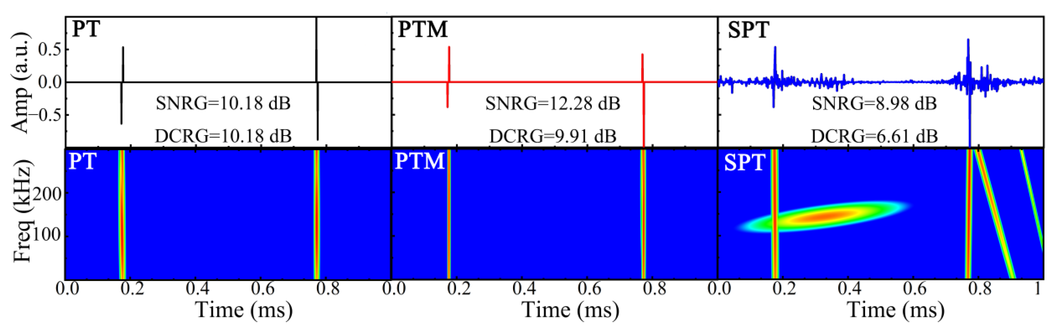
The optimized synthesized UGW signals processed by FBR-RC-SSP are shown in Figure 10. It can be observed that only defect and end-reflected echoes are retained, of which the amplitudes of defect echoes are the same as that of the synthesized UGW signal. In addition, PT and PTM show an excellent coherent noise elimination effect: their SNRGs are 10.18 dB and 12.2 dB, and DCRGs are 10.18 dB and 9.91 dB, while the coherent noise of SPT still can be found clearly in the time-frequency domain.

5. Simulations of UGW Testing

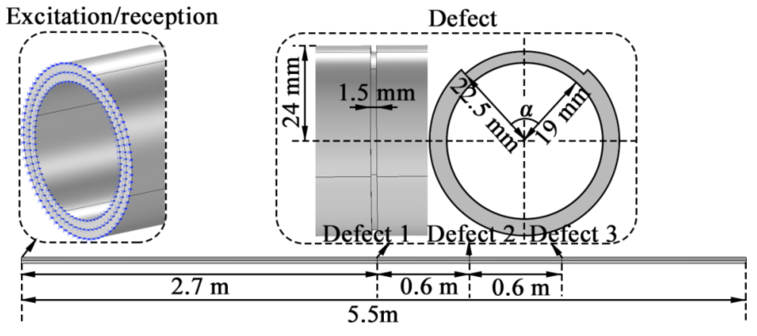
Comsol Multiphysics software was used to simulate the UGW testing, and the pipeline model was built, as illustrated in Figure 11. The pipe length is 5.5 m, the outer diameter is 48 mm, and the thickness is 5 mm. Defect 1 is 2.7 m away from the excitation/reception end, and the spacing among defects is 0.6 m. 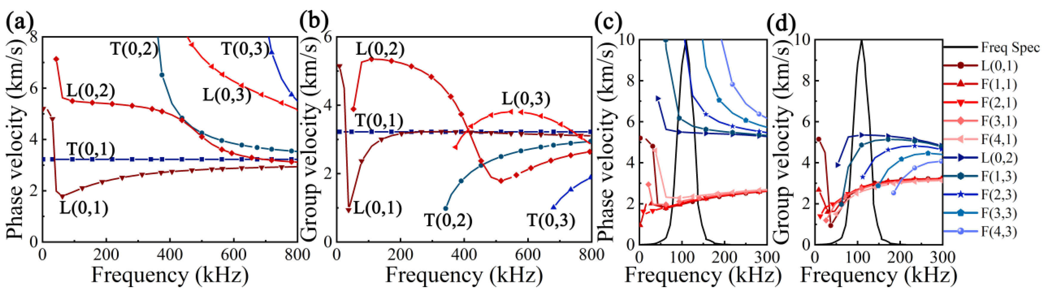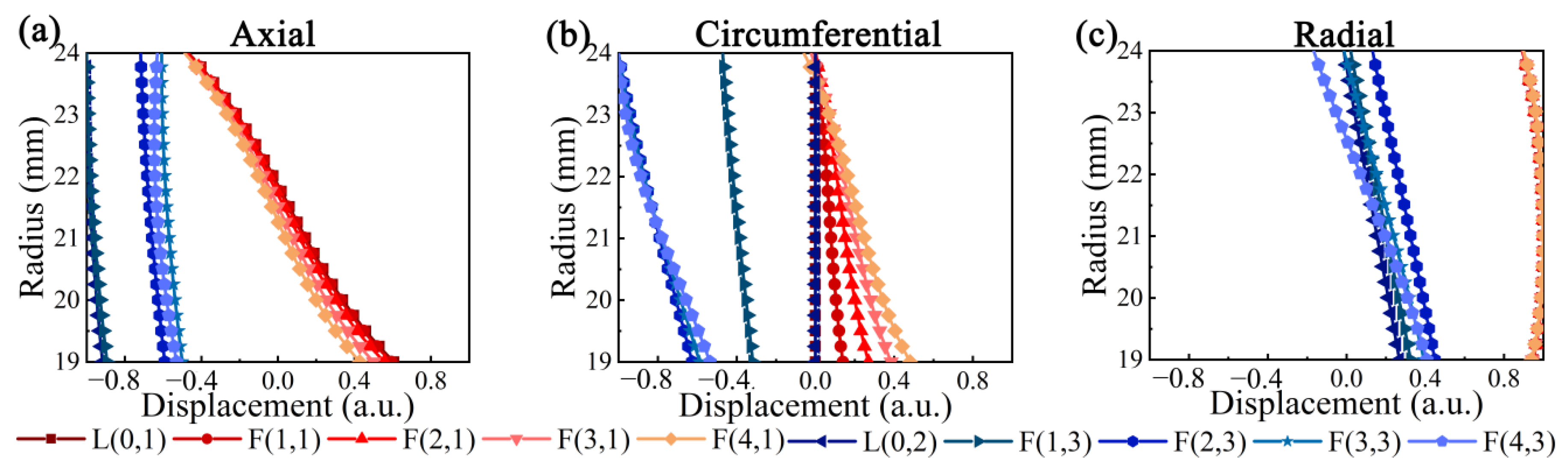The pipe material is low-carbon steel, and the density, Young’s modulus and Poisson’s ratio are 7.89 g/cm³, 200 GPa and 0.27, respectively. The circumferential angle of the defect is α, and the depth and width of the defect are both 1.5 mm. At the excitation/reception end, 65 points were taken at r = 19 mm, 21.5 mm and 24 mm (r is the radius of the pipe) at equal distances along the circumference, respectively, of which the sinusoidal signals modulated by a 5-period Hanning window and the wave structure of L(0,2) UGW at 110 kHz were input to each excitation point from axial, circumferential and radial directions, and 65 points along the circumferential direction of r = 24 mm were taken as the receiving points.

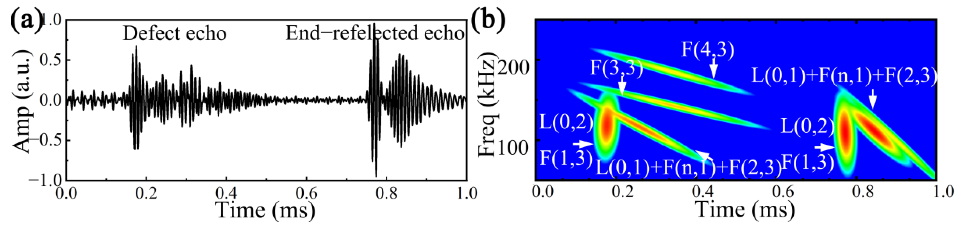
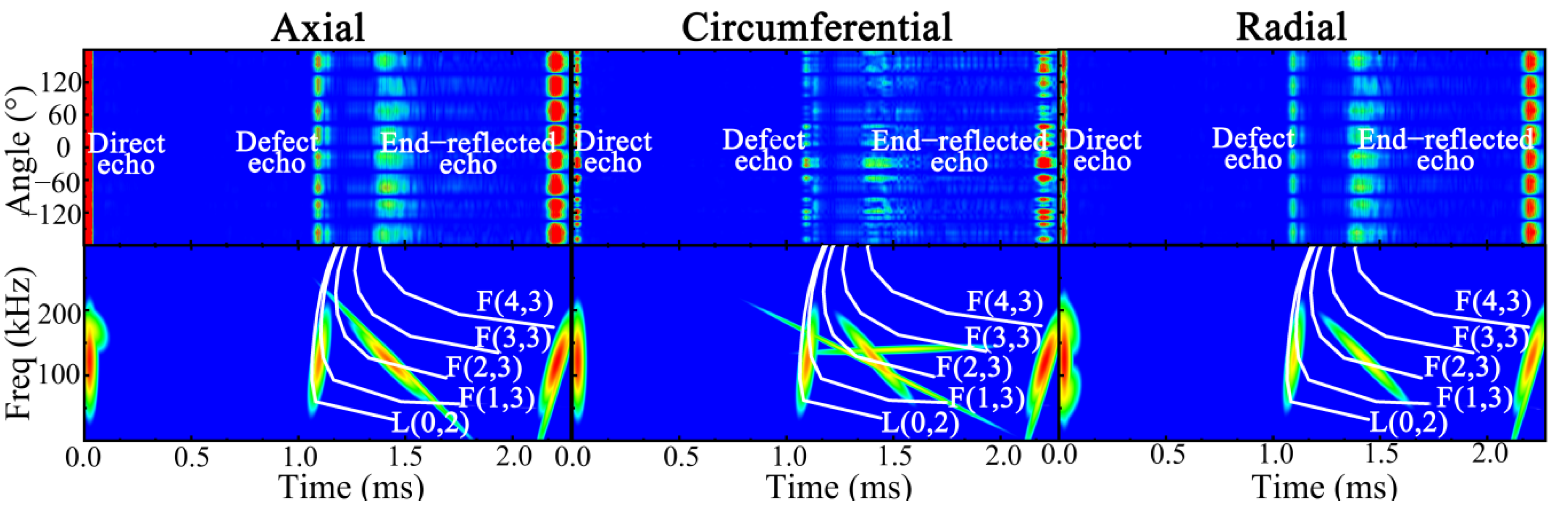
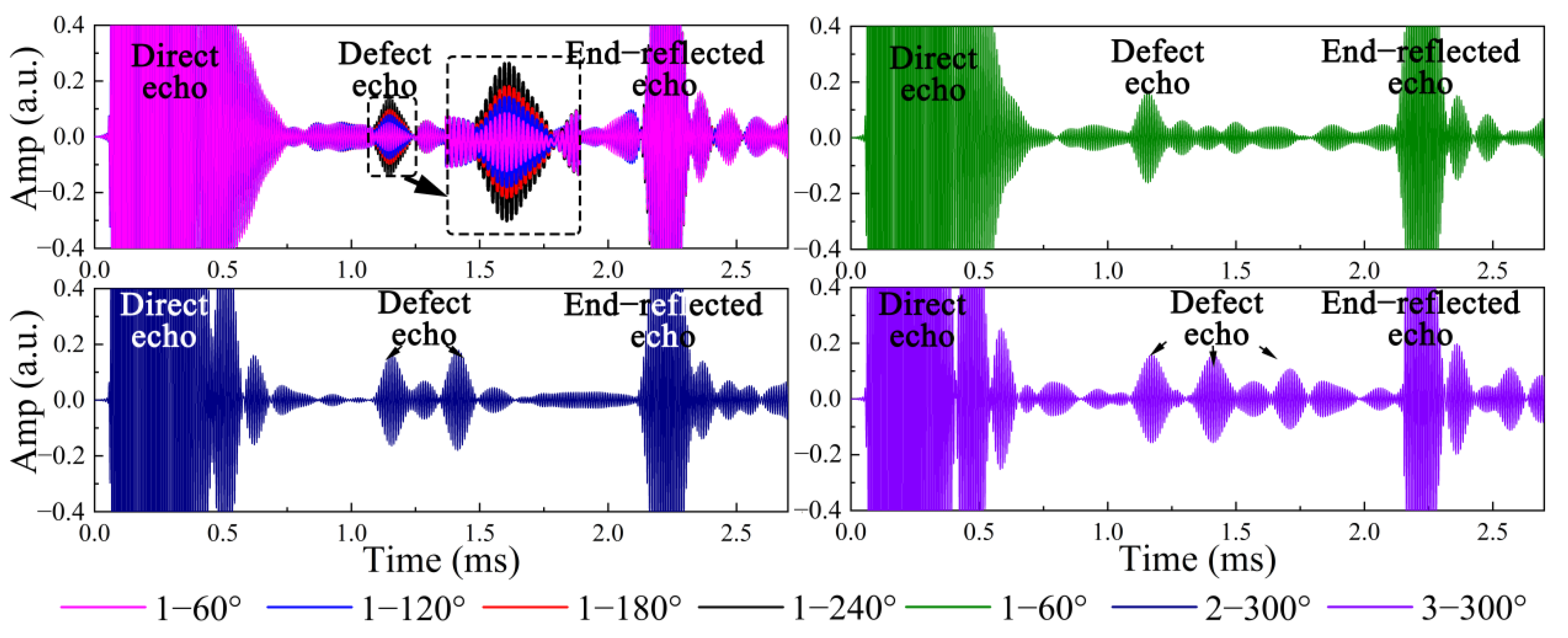
The simulated UGW signals with 1 defect (α = 300°) are shown in Figure 12. It can be seen from the signals in the time domain that the direct and end-reflected echoes with great amplitudes are obvious, and the resolution of defect is weak because of the influence of coherent noise, especially the circumferential signals. It can be observed from the signals in the frequency domain that F(1,3) and F(2,3) UGWs arise in the axial and radial directions when L(0,2) UGW encounters the asymmetric defect, wheras the F(1,3), F(2,3) and F(3,3) UGWs appear in the circumferential direction. 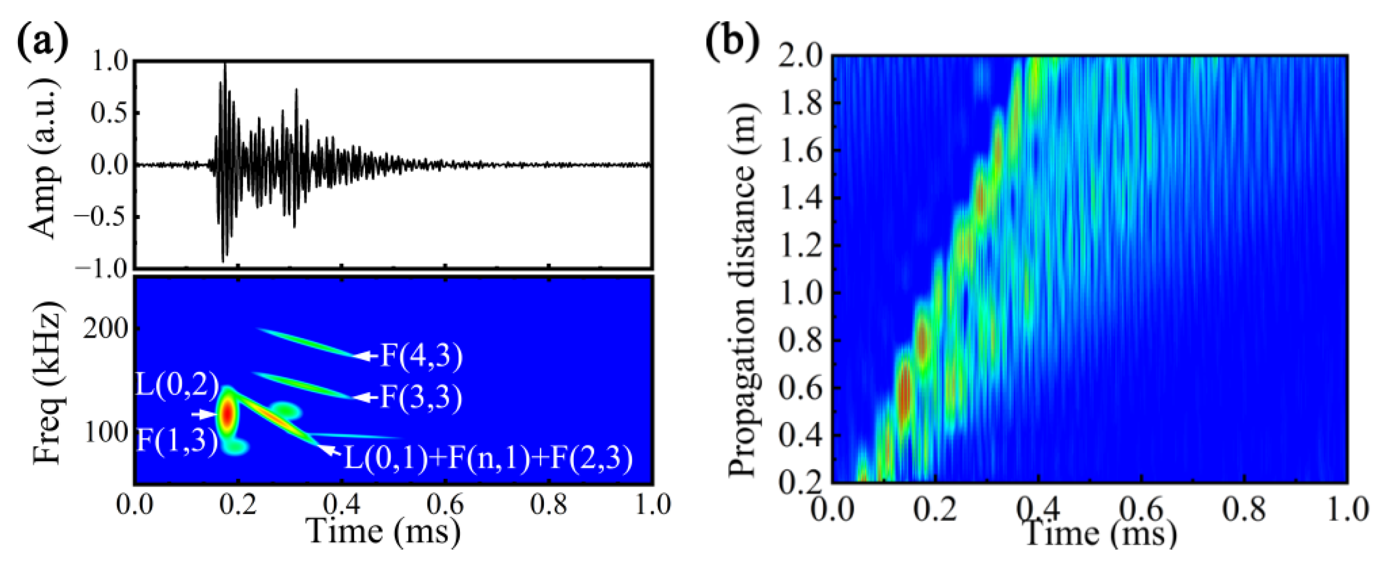This may be because the biggest difference among L(0,2) and F(n,3) UGWs is the circumferential displacement. Considering that L(0,2) UGW is dominated by the axial displacement, the simulated UGW signals below are represented by the axial displacement signals.

The simulated UGW signals with a multi-defect (α = 300°) are shown in Figure 13. It is predictable that the L(0,2) UGW undergoes multiple mode conversions at defects when there are multiple defects in the pipeline, resulting in more coherent noise in the signal. Moreover, the amplitude of the defect echo may decrease because of the increase in the defect number with the consistent excitation energy. It is possible to confuse the defect signals with coherent noise and even give the wrong detection. In addition, it can also be observed that the chirplet transform shows the limitation of distinguishing defects when there are three defects; this is true for frequency domain signals obtained by the chirplet transform with high resolution, not to mention the time domain signals.

Comsol Multiphysics software was used to simulate the UGW signals with different number and circumferential angle α, the data of 65 receiving points were averaged and the results are illustrated in Figure 14, where 3–300° indicates that there are three defects and α = 300°. It can be seen that the amplitudes of the defect echo and coherent noise become big as α increases from 60° to 300°, which is caused by the greater energy reflected from the defect with a larger cross-sectional area loss. In addition, it is similar to Figure 13 in that the defect echoes are polluted by the coherent noise when there are three defects; so, the signal interpretation accuracy decreases.

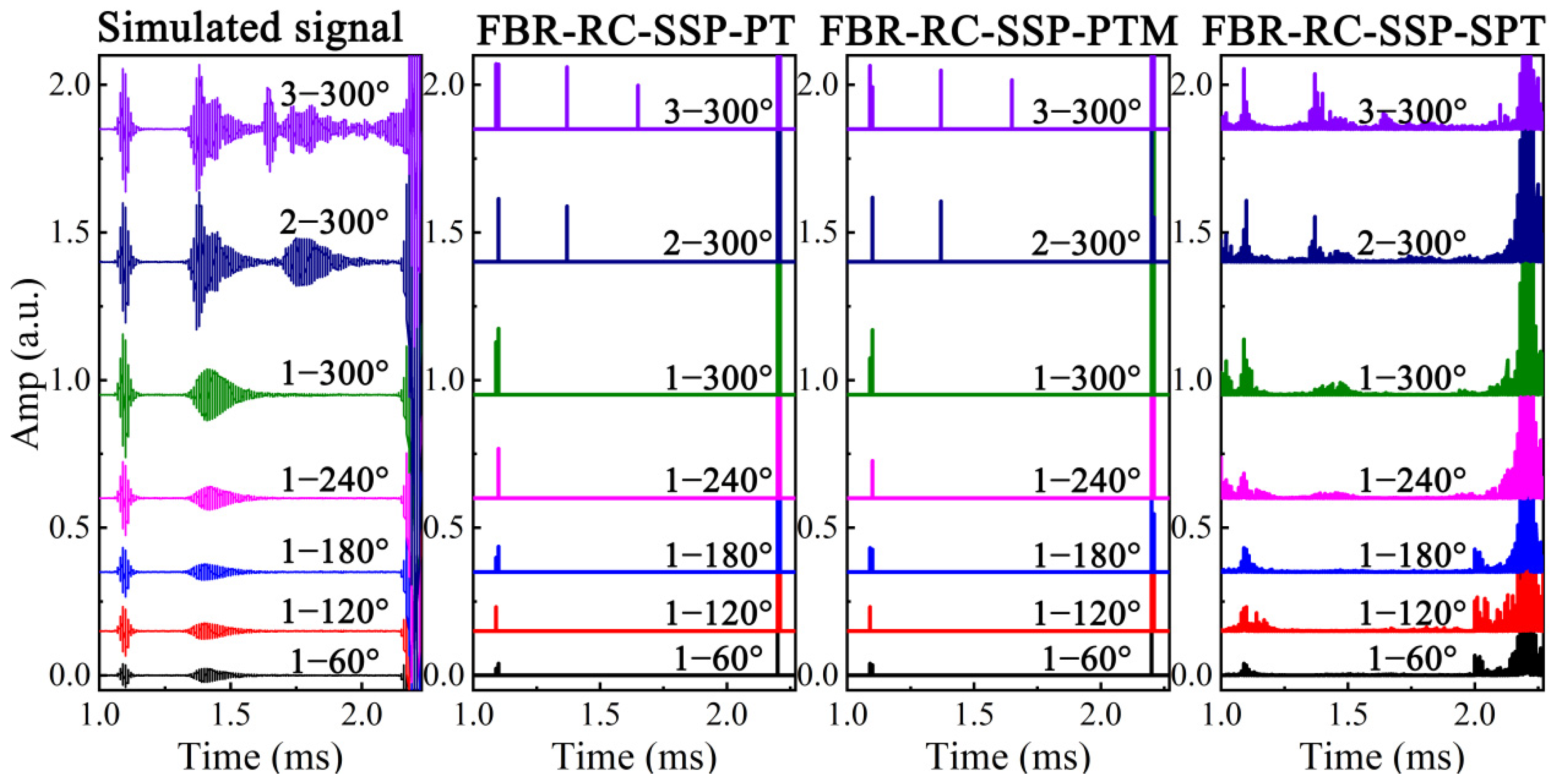
FBR-RC-SSP was applied to the above signals, the corresponding SNRGs and DCRGs were calculated and the results are shown in Figure 14 and

Table 2. SNRGs and DCRGs of simulated UGW signals processed by FBR-RC-SSP.

	FBR-RC-SSP-PT		FBR-RC-SSP-PTM		FBR-RC-SSP-SPT
	SNRG (dB)	DCRG (dB)	SNRG (dB)	DCRG (dB)	SNRG (dB)	DCRG (dB)
1–60°	15.07	14.15	15.08	14.14	7.50	7.37
1–120°	12.73	11.95	14.73	14.15	6.22	5.24
1–180°	12.70	12.05	14.84	13.85	6.67	6.48
1–240°	12.66	13.85	13.07	12.84	4.82	3.88
1–300°	13.33	13.57	14.84	14.09	5.57	5.19
2–300°	13.78	13.96	13.07	12.18	6.03	5.16
3–300°	12.12	12.96	13.94	12.13	6.04	5.13
Mean	13.19	13.21	14.22	13.34	6.12	5.49

. It can be observed that FBR-RC-SSP-SPT show the worst processing effect. Although it can retain the defect and end-reflected echoes and the signal resolution is improved to a certain extent—where the average SNRG and DCRG are 6.12 dB and 5.49 dB, respectively—there are still coherent noises in the signals making it difficult to locate and quantify defects. The processing effects of FBR-RC-SSP-PT and PTM are similar: both defect and end-reflected echoes are clearly displayed with almost no coherent noise (the average SNRGs are 13.19 dB and 14.22 dB, and the average DCRGs are 13.21 dB and 13.34 dB, respectively). Therefore, it is logical to choose PT and PTM as the signal recombination methods in UGW testing, which makes signal interpretation very convenient. The following sections focus on these two methods.

6. Experiments of UGW Testing

UGWs can be excited and received based on the principles including but not limited to piezoelectricity, magnetostriction, electromagnetism and laser. Magnetostrictive UGW testing has ease of implementation, low cost, excellent sensitivity and durability, and has been widely used in the nondestructive testing of pipelines [27,28]. The magnetostrictive effect is a coupling phenomenon involving the magnetization and the size/shape change of ferromagnetic material; an UGW could be excited by the positive magnetostrictive effect, which is reflected or refracted at pipe discontinuities or defects, and received by the inverse magnetostrictive effect, which can be analyzed to determine whether a defect exists [29,30].

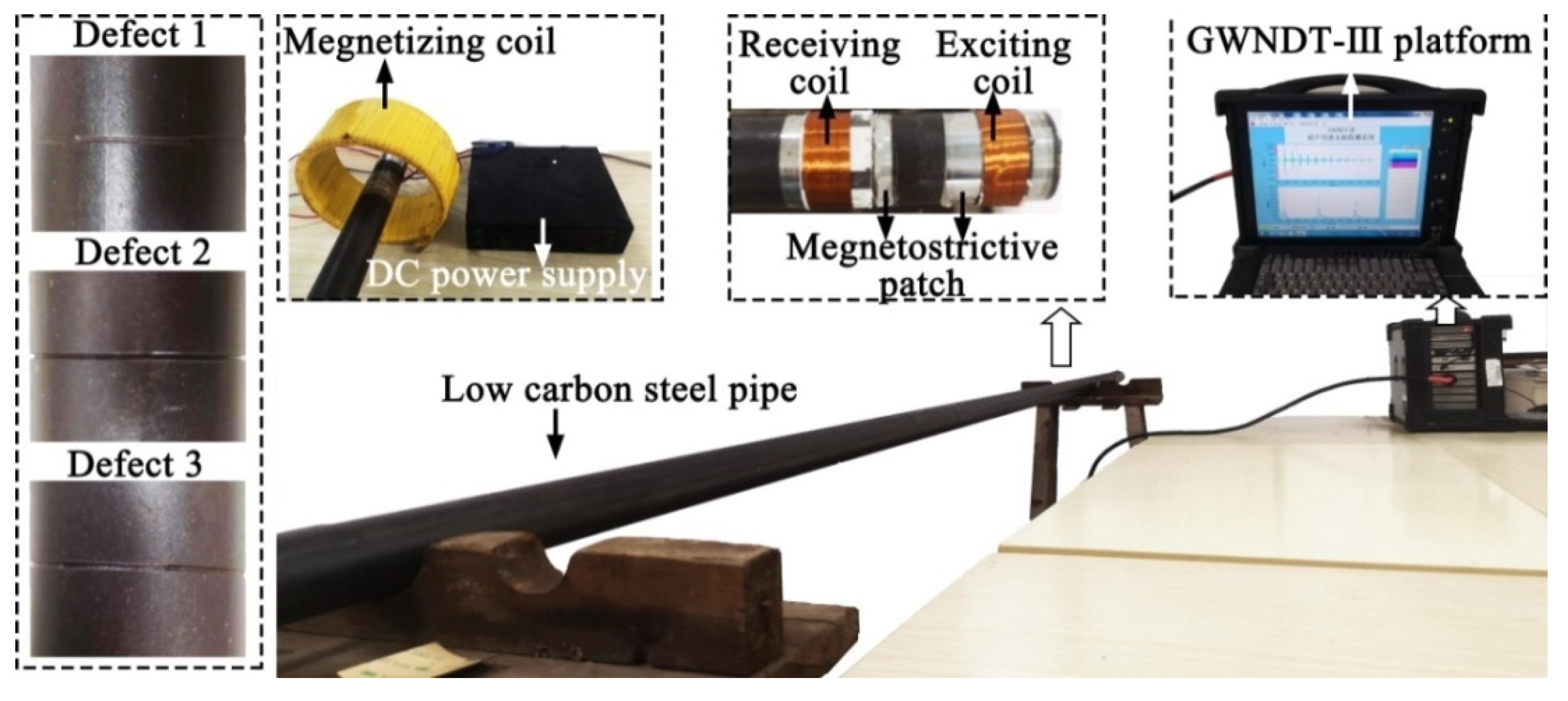
To perform magnetostrictive UGW testing in this study, we developed a platform called GWNDT-III, which can generate excitation signals modulated by a power amplifier module and collect received signals modulated by a signal processing module, as illustrated in Figure 15. In order to excite as pure an L(0,2) UGW at 110 kHz as possible, the length of excitation coil l_c should be calculated by l_c = 0.5V_p/f_c [31] (V_p is the phase velocity, f_c is the central frequency).

The utilized pipe was the same as the one used in simulation. The static bias and dynamic alternating magnetic fields were provided by a magnetostrictive patch (FeCo alloy) and an excitation coil, where the parameters of the excitation and receiving coils were the same and the magnetostrictive patch was bonded with the pipe using epoxy resin. Furthermore, the magnetostrictive patch was magnetized using a magnetizing coil through which direct current was passed, and the excitation coil was supplied with 20 V alternating voltage and placed at one end of the pipe in order to ensure that the UGW propagates in one direction; the distance between the excitation and receiving coils was 40 mm.

The experimental UGW signals with different defect circumferential angles and numbers were obtained by GWNDT-III, as shown in Figure 16. It can be seen that the direct echo is wider and the signal resolution is lower compared with those of simulated UGW signals. The degree of distinction from coherent noise is not obvious for the low amplitude of the defect echo when 60° ≤ α ≤ 180°, and this phenomenon may also occur when there are two or three defects, which may lead to the wrong detection result and further reduce the signal interpretation accuracy.

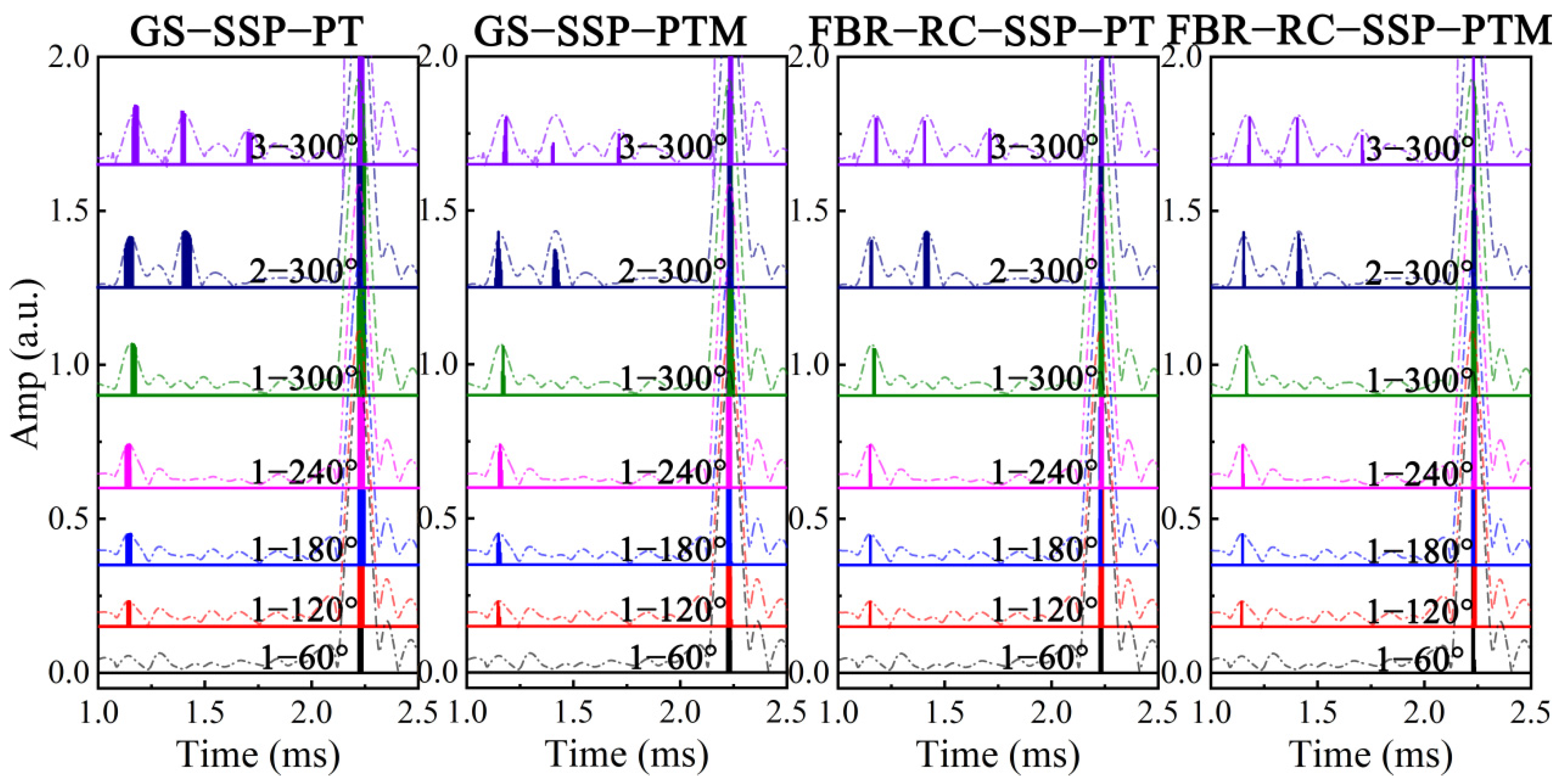
GS-SSP and FBR-RC-SSP were applied to the experimental UGW signals (1–2.5 ms), and the results are illustrated in Figure 17, where the dotted lines are the packet of the unprocessed experimental UGW signals. The SNRGs and DCRGs of the processed experimental UGW signals are as shown in

Table 3. SNRGs and DCRGs of experimental UGW signals processed by FBR-RC-SSP.

	GS-SSP-PT		GS-SSP-PTM		FBR-RC-SSP-PT		FBR-RC-SSP-PTM
	SNRG(dB)	DCRG(dB)	SNRG(dB)	DCRG(dB)	SNRG(dB)	DCRG(dB)	SNRG(dB)	DCRG(dB)
1–60°	16.27	-	18.15	-	18.79	-	20.82	-
1–120°	15.25	15.04	15.92	15.66	17.23	17.81	18.83	18.27
1–180°	14.31	15.21	17.71	17.56	19.45	19.11	20.20	20.05
1–240°	15.16	15.06	16.55	16.43	17.21	17.95	18.86	18.46
1–300°	13.87	13.31	14.19	13.54	16.59	16.14	18.39	18.40
2–300°	14.59	15.20	15.78	15.01	19.25	18.65	18.89	18.51
3–300°	14.12	14.06	16.65	16.58	20.81	20.28	22.97	22.16
Mean	14.79	14.64	16.42	15.79	18.48	18.32	19.85	19.31

. Both GS-SSP and FBR-RC- SSP can eliminate the coherent noise and improve the signal resolution, of which PTM shows a slightly better effect compared with that of PT. Compared with GS-SSP, FBR-RC-SSP exhibits better effects of improving the signal interpretation accuracy: the average SNRG (19.17 dB) and DCRG (18.82 dB) are larger, which have increased by about 22.92% and 23.71%. However, FBR-RC-SSP shows a limitation when the DCR of the UGW signal (1–60°) is too low, and it could not distinguish the defect echo sensitively, as the defect echo is completely submerged by the coherent noise, which was also discussed in the study of Pedram et al. [23]. In addition, the defect echo amplitude may change after the processing of SSP, which is very obvious in GS-SSP-PTM, but the defect echo amplitude before and after applying FBR-RC-SSP could be kept the same. In summary, FBR-RC-SSP is conducive to improving the signal resolution and has the potential to help the further location and quantitative analysis of defect.

7. Conclusions

Split-spectrum processing with raised cosine filters of constant frequency-to-bandwidth ratio (FBR-RC-SSP) was proposed to improve the signal interpretation accuracy of L(0,2) ultrasonic guided wave (UGW) testing. The chirplet transform for time-frequency analysis was used to study the dispersion and multi-mode of the synthesized UGW signal (L(0,1) + L(0,2) + F(n,1) + F(n,3), 1 ≤ n ≤ 4). The signal-to-noise ratio gain (SNRG) and defect-to-coherent noise gain (DCRG) were introduced to reveal the effects of filter parameters on SNRG and DCRG, and the processing effects of FBR-RC-SSP were verified by the simulated and experimental UGW signals.

Unlike the Gaussian (GS) filters, the raised cosine (RC) filters have transition bands in the shape of a truncated raised cosine cycle, and the energy contained in the RC filter is mostly concentrated around the center frequency for the flat top design. In addition, FBR-RC filters have a wider bandwidth compared with those of RC filters and the resolution of time pulse is higher. It is therefore easy to foresee that FBR-RC filters can better meet the requirements of minimizing the degree of overlap without losing substantial information compared with GS filters.

In order to obtain the best processing effect, it is necessary to choose the appropriate filter parameters (total bandwidth B, transition bandwidth B_t, flat top width B_r, filter spacing Δf) for the parameter sensitivity of SSP. Only defect and end-reflected echoes were retained in the synthesized, simulated and experimental UGW signals processed by FBR-RC-SSP, while the coherent noise was eliminated, and the signal interpretation accuracy was improved. In addition, Polarity Thresholding (PT) and Polarity Thresholding with Minimization (PTM) were the suitable signal recombination methods for L(0,2) UGW testing. In this way, the average SNRG and DCRG of FBR-RC-SSP were about 22.92% and 23.71% higher than the traditional GS-SSP, which may be meaningful to the further location and quantitative analysis of defect.