Article

Quasi-Consensus of Disturbed Nonlinear Multiagent Systems with Event-Triggered Impulsive Control

School of Automation, Guangdong University of Technology, Guangzhou 510006, China
*
Author to whom correspondence should be addressed.
Appl. Sci. 2022, 12(15), 7580; https://doi.org/10.3390/app12157580
Submission received: 1 April 2022 / Revised: 15 July 2022 / Accepted: 22 July 2022 / Published: 28 July 2022

Abstract

:
Considering the external disturbances, in this paper, the quasi-consensus of multiagent systems is studied via event-triggered impulsive control. By designing a novel event-triggered mechanism (ETM), sufficient conditions to realize leader-following quasi-consensus are derived with event-triggered impulsive control. Additionally, Zeno behavior is also excluded. It is shown that the event-triggered frequency is closely related to the parameters selected in the designed ETM, and less conservative results can be obtained compared with the existing results. Finally, a simulation example is given to demonstrate the effectiveness of our proposed results.

1. Introduction

Owing to the wide applications of multiagent systems (MASs) in practice, its related research has attracted great attention from scholars. Cooperative control technology is an important issue of MASs, which are widely used in the fields of unmanned aerial vehicle formation [1], power systems [2], cluster robots [3] and so on. Moreover, consensus is one of the most popular issues of cooperative control technology, and the related research has achieved fruitful results so far [4,5,6,7]. The general concept of consensus, however, cannot tolerate any interference. To tackle the effect of external disturbance or attack, the quasi-consensus is proposed. The concept of quasi-consensus is used to describe the effects caused by the interference, and the error state is finally within a bound corresponding to the interference above, instead of zero, as the time tends to infinity. It is great significance when the MASs encounter some inevitable environmental or artificial disturbance in practical applications. For example, Hu [8] studied the quasi-consensus of second-order MASs with external disturbances, and Ma [9] studied the quasi-consensus of discrete-time time-varying MASs with randomly occurring nonlinearities (RONs) and deception attacks, where the RONs were first studied in [10]. In MASs, according to whether there is a leader or not, they can be divided into leader-following and non-leader-following consensuses. The consensus of leader-following is closer to reality, which is a hot topic in the current research. Almeida [11] studied the leader-follower consensus of fractional MASs, and Liu [12] studied the leader-following consensus of MASs with switched networks.
It is worth noting that MASs are usually in a complex and changeable engineering environment, and the evolution process of the system is affected by the surrounding environment, such as the uncertainty of system parameters and the change in system nonlinear dynamics caused by environmental impact. These objective phenomena may seriously affect the evolution process of the system. Considering randomly occurring uncertainties (ROUs) and RONs, robustness of systems are discussed [13]. At present, many scholars have studied MASs with ROUs and RONs and achieved many excellent research results [14,15,16,17].
Considering the communication load and control cost, the selection and design of control strategy are very important in the research on the consensus of MASs. At the beginning, scholars used continuous control to make the MASs realize consensus, such as including control [18], adaptive control [19], pinning control [20], etc. Although continuous control is relatively simple, continuous control requires the controller to work all the time, which leads to a waste of resources. To solve this problem, scholars proposed impulsive control, but the impulsive sequence is generally set and selected manually in advance. Impulsive control has been widely used in the control field because of its low control cost, strong robustness and good confidentiality. For examples, using impulsive control method, Li [21] studied the stabilization of delayed systems; Zhang [22] investigated the synchronization of delayed neural networks; and Yang [23] considered the consensus of delayed MASs with random disturbances. However, because the impulsive sequence is artificially set, it may be too conservative a lead to increase unnecessary control times.
To solve these shortcoming, the event-triggered mechanism (ETM) [24,25,26,27] was proposed. The control sequence depends on some triggering conditions according to the system state and so on. Compared with time-triggered impulsive control, event-triggered impulsive control (ETIC) combines both the event-triggered strategy and impulsive control, and hence, ETIC can effectively reduces the cost of control [28,29,30,31]. At present, scholars attach great importance to the research of ETIC strategy. For instant, using ETIC, the consensus of linear MASs [28], synchronization of neural networks [30] and complex dynamic networks [29] were investigated.
Inspired by the above discussion, based on the ETIC strategy, this paper studies the quasi-consensus of nonlinear MASs with various obstructions (ROUs, RONs and external disturbances). The main contributions are as follows:
  • In this paper, various obstructions are considered. Compared with the works in [31], the stochastic characteristics of uncertainties, i.e., ROUs and RONs, are considered. Moreover, the external disturbances in the leader and followers here can be different. Hence, the system model is more general and practical.
  • The ETM designed in this paper is antidisturbance compared with the existing results [32,33,34]. Additionally, differently from the one in [31], the effects of disturbances are intuitive, which makes it easier to adjust for various disturbances.
Notation 1.
N + , R and R n are defined as the set of positive integers, the set of real numbers and the n-dimensional Euclidean space, respectively. By A B , we mean that A B is a seminegative definite matrix. A T denotes the transposition of matrix A, represents the Kronecker product, · represents both the induced matrix 2-norm and the usual Euclidean vector norm. λ max ( A ) stands for the maximum eigenvalue of the matrix A. E [ · ] denotes the mathematical expectation and P r { B } is the probability of the event B. I n represents the n-dimensional identity matrix.
The rest of this paper is organized as follows. Preliminaries are given in Section 2. The main results and the constructed ETM are established in Section 3. Section 4 gives an example to verify the derived results, and Section 5 concludes this paper.

2. Preliminaries and Model Description

2.1. Graph Theory

In MASs, the communication among agents can be reflected by the graph. Each agent can be seen as a node, and let V = { v 1 , v 2 , , v N } be the node set. Let E V × V be the edge set, and the undirected topology of MASs can be described by the graph G = ( V , E , C ) , where C = [ a i j ] N × N represents the adjacency matrix of G. If ( i , j ) E , it means that agents i and j do not communicate with each other, there are a i j = a j i = 0 , otherwise a i j = a j i = 1 . Additionally, define a i i = 0 . D = diag ( d 1 , d 2 , , d N ) is defined as the degree matrix of G, where d i = j = 1 , j i N a i j . L = [ l i j ] N × N is called the Laplacian matrix of G and L = D C . The communication state between leader and followers are represented by a matrix B = diag ( b 1 , b 2 , , b N ) . If the follower can communicate with the leader, then b i = 1 , otherwise b i = 0 . We call N i : = { j | a i j > 0 } the neighbor set of agent i. Let H = L + B . N i is defined as the set of agents that communicate with the agent i. If a node can reach any nodes in the graph, then the node is called the root, and the graph has a spanning tree with the root.

2.2. The Mathematical Model of Leader-Following MASs

Consider the MASs consist of one leader and N followers, and each agent suffers from the ROUs, RONs and external disturbance. The dynamics of the i-th ( i = 1 , 2 , , N ) follower is:
x ˙ i ( t ) = A ( t ) x i ( t ) + β ( t ) f ( t , x i ( t ) ) + w i ( t ) + u i ( t ) , t t 0 , x i ( t 0 ) = φ i ,
where t 0 0 is the initial instant and φ i R n is the initial value of the i-th follower. x i ( t ) R n is the system state, u i ( t ) R n is the control input and w i ( t ) R n denotes the external disturbance. A ( t ) = A + α ( t ) M P ( t ) Q , where A , M and Q are suitable constant matrices. P ( t ) is time-varying matrix and satisfies P ( t ) P T ( t ) I n . f : R × R n R n is a nonlinear function. β ( t ) f ( · ) and α ( t ) M P ( t ) Q are used to describe the uncertain information of the system and nonlinearities that may occur randomly (i.e., RONs and ROUs) in practical application, respectively. Additionally, assume that α ( t ) and β ( t ) satisfy Assumption 2.
Let x 0 ( t ) R n denote the state of the leader, whose dynamic is described as:
x ˙ 0 ( t ) = A ( t ) x 0 ( t ) + β ( t ) f ( t , x 0 ( t ) ) + w 0 ( t ) , t t 0 , x 0 ( t 0 ) = φ 0 ,
where φ 0 R n is the initial value of the leader.
To realize the quasi-consensus of the above MASs, the following impulsive protocol is designed:
u i ( t ) = k = 1 + μ k ( j N i a i j ( x i ( t ) x j ( t ) ) + b i ( x i ( t ) x 0 ( t ) ) ) δ ( t t k ) ,
where μ k R is the impulsive gain, and δ ( t ) is the Dirac delta function which is used to model the impulsive dynamic [35]. { t k , k N + } is the impulsive control sequence generated by the ETM to be designed.
Combining (1) and (3), one can obtain that
x ˙ i ( t ) = A ( t ) x i ( t ) + β ( t ) f ( t , x i ( t ) ) + w i ( t ) , t t k , Δ x i ( t k ) = x i ( t k + ) x i ( t k ) = μ k j N i a i j ( x i ( t k ) x j ( t k ) ) + μ k b i ( x i ( t k ) x 0 ( t k ) ) , t = t k , x i ( t 0 ) = φ i ,
where x i ( t ) at t k is right continuous, with x i ( t k ) = x i ( t k + ) being assumed. Δ x i ( t k ) represents the jump value at t = t k .
Then, according to (4), we construct the following error system:
e ˙ i ( t ) = A ( t ) e i ( t ) + β ( t ) g ( t , e i ( t ) ) + w ˜ i ( t ) , t t k , Δ e i ( t k ) = e i ( t k + ) e i ( t k ) = μ k j N i a i j ( e i ( t k ) e j ( t k ) ) + μ k b i e i ( t k ) , t = t k , e i ( t 0 ) = φ i φ 0 ,
where e i ( t ) = x i ( t ) x 0 ( t ) , w ˜ i ( t ) = w i ( t ) w 0 ( t ) , g ( t , e i ( t ) ) = f ( t , x i ( t ) ) f ( t , x 0 ( t ) ) .
Let e ( t ) = [ e 1 T ( t ) , e 2 T ( t ) , , e N T ( t ) ] T , G ( t , e ( t ) ) = [ g T ( t , e 1 ( t ) ) , g T ( t , e 2 ( t ) ) , , g T ( t , e N ( t ) ) ] T , w ˜ ( t ) = [ w ˜ 1 T ( t ) , w ˜ 2 T ( t ) , , w ˜ N T ( t ) ] T and 1 N be the N-dimensional vector with all elements equal to one. Using the Kronecker product, the error system (5) can be rewritten as the following compact form:
e ˙ ( t ) = ( I N A ( t ) ) e ( t ) + β ( t ) G ( t , e ( t ) ) + w ˜ ( t ) , t t k , Δ e ( t k ) = μ k ( H I n ) e ( t k ) , t = t k , e ( t 0 ) = 1 N ( φ i φ 0 ) ,

2.3. Some Definitions, Lemmas and Assumptions

Definition 1
([31]). The leader-following MASs consist of (1) and (2) is said to achieved quasi-consensus if e ( t ) converges into a bounded set B as t + ,
B = e ( t ) R N n | E [ e ( t ) 2 ] χ ,
where χ > 0 is called the error bound.
Definition 2
([36]). Given a function ϕ : R R , define the upper-right-hand Dini derivative of
D + ϕ ( t ) = lim sup l 0 + ( ϕ ( t + l ) ϕ ( t ) ) l .
Lemma 1
([15]). For any p , q R n and η > 0 , the following inequality holds:
p T q + q T p η p T p + η 1 q T q .
Assumption 1.
The nonlinear function f in (1) and (2) satisfies the following Lipchitz condition:
f ( t , p ) f ( t , q ) J ( p q ) ,
where p , q R n , and J R n × n is a constant matrix.
Assumption 2.
The time-varying parameters β ( t ) and α ( t ) in system (1) are independent of each other and obey the Bernoulli distribution, meeting the following conditions: E [ α ( t ) ] = α ¯ and E [ β ( t ) ] = β ¯ , where α ¯ , β ¯ [ 0 , 1 ] .
Assumption 3.
The communication topology of MASs has a spanning tree with the leader as the root node.
Assumption 4.
w ˜ ( t ) in (6) is bounded and it satisfies sup t t 0 w ˜ ( t ) w < + .

3. Main Results

In this section, we derive some sufficient conditions to ensure the quasi-consensus of the considered MASs using ETIC strategy. Additionally, we show that Zeno behavior is excluded. First, the ETM is designed as follows:
t k = min { t k * , t k 1 + τ sup } , t k * = inf t > t k 1 | E [ V ( e ( t ) ) ] e l k λ ( t t k 1 ) E [ V ( e ( t k 1 ) ) ] + υ w 2 ,
where τ sup > 0 is the maximum allowable event-trigger interval to be designed; l k > 0 , k N + , υ > 1 and λ > 0 . V ( e ( t ) ) is the Lyapunov function to be defined with respect to e ( t ) .
Remark 1.
With the help of impulsive control, information transmission in the designed ETM can only activate at triggered instants. In other words, there is no need for any information transmission during the event-triggered interval, which can effectively reduce the communication cost.
Remark 2.
Compared with the anti-disturbance ETM in [31], where the effects of disturbances are hidden in some parameters, they are intuitive in our designed ETM. The sensitivity of the ETM (9) to disturbances can be adjusted by the parameter υ. Moreover, the measuring error, i.e., e ( t ) e ( t k 1 ) for any t [ t k 1 , t k ) , k N + used in [31] is no longer needed, which can also cut down the communication or computing resources in some sense.
Remark 3.
The forced impulse generated by the event t k 1 + τ sup is to ensure the existence of the maximum allowable event-trigger interval. Note that it is important for achieving quasi-consensus of MASs, since one can always derive an upper bound of τ sup by the following theorem.
Theorem 1.
Suppose that Assumptions 1–4 are satisfied. If there exist constants η 1 , η 2 > 0 such that
0 < σ < 1 , θ = ln σ τ sup + ρ < 0 ,
where
ρ = λ max ( Λ ) + 2 β ¯ J + η 2 , Λ = I N ( A + A T + α ¯ η 1 M M T + α ¯ η 1 1 Q T Q ) , σ = sup k N + λ max ( ( μ k H T I n + I N n ) ( μ k H I n + I N n ) ) .
Then, under the impulsive controller (3), the leader-following MASs consisting of (1) and (2) achieve quasi-consensus with the estimated error bound:
χ = 4 w 2 | θ | σ η 2 .
Proof
Select the following Lyapunov function:
V ( e ( t ) ) = e T ( t ) e ( t ) .
The derivative of (11) along (6) can be obtained:
D + V ( e ( t ) = e T ( t ) e ˙ ( t ) + e ˙ T ( t ) e ( t ) = e T ( t ) [ ( I N A ( t ) ) T + ( I N A ( t ) ) ] e ( t ) + β ( t ) G T ( t , e ( t ) ) e ( t ) + β ( t ) e T ( t ) G ( t , e ( t ) ) + e T ( t ) w ˜ ( t ) + w ˜ T ( t ) e ( t ) = e T ( t ) [ I N ( A T + A ) ] e ( t ) + w ˜ T ( t ) e ( t ) + 2 e T ( t ) [ I N α ( t ) M P ( t ) Q ] e ( t ) + 2 β ( t ) G T ( t , e ( t ) ) e ( t ) + e T ( t ) w ˜ ( t ) .
According to Lemma 1 and Assumption 1, we obtain:
2 e T ( t ) [ I N α ( t ) M P ( t ) Q ] e ( t ) = 2 e T ( t ) [ I N α ¯ M P ( t ) Q ] e ( t ) + 2 e T ( t ) [ I N ( α ( t ) α ¯ ) M P ( t ) Q ] e ( t ) e T ( t ) [ I N α ¯ ( η 1 M M T + η 1 1 Q T Q ) ] e ( t ) + 2 e T ( t ) [ I N ( α ( t ) α ¯ ) M P ( t ) Q ] e ( t ) ,
and
2 β ( t ) G T ( t , e ( t ) ) e ( t ) + e T ( t ) w ˜ ( t ) + w ˜ T ( t ) e ( t ) = 2 β ¯ G T ( t , e ( t ) ) e ( t ) + 2 ( β ( t ) β ¯ ) G T ( t , e ( t ) ) e ( t ) + e T ( t ) w ˜ ( t ) + w ˜ T ( t ) e ( t ) ( 2 β ¯ J + η 2 ) e T ( t ) e ( t ) + η 2 1 w ˜ T ( t ) w ˜ ( t ) + 2 ( β ( t ) β ¯ ) G T ( t , e ( t ) ) e ( t ) .
Combining (12)–(14), we have
D + V ( e ( t ) ) e T ( t ) [ I N ( A + A T ) ] e ( t ) + α ¯ e T ( t ) [ I N ( η 1 M M T + η 1 1 Q T Q ) ] e ( t ) + 2 e T ( t ) [ I N ( α ( t ) α ¯ ) M P ( t ) Q ] e ( t ) + 2 ( β ( t ) β ¯ ) G T ( t , e ( t ) ) e ( t ) + ( 2 β ¯ J + η 2 ) e T ( t ) e ( t ) + η 2 1 w ˜ T ( t ) w ˜ ( t ) ρ V ( e ( t ) ) + η 2 1 w ˜ T ( t ) w ˜ ( t ) + 2 e T ( t ) [ I N ( α ( t ) α ¯ ) M P ( t ) Q ] e ( t ) + 2 ( β ( t ) β ¯ ) G T ( t , e ( t ) ) e ( t ) .
When t [ t k 1 , t k ) , k N + , V ( e ( t ) ) is continuous, the following equation holds:
E [ V ˙ ( e ( t ) ) ] = D + E [ V ( e ( t ) ) ] ,
which indicates that:
E [ V ˙ ( e ( t ) ) ] ρ E [ V ( e ( t ) ) ] + η 2 1 w ˜ T ( t ) w ˜ ( t ) ,
where ρ = λ max ( Λ ) + 2 β ¯ J + η 2 , and Λ = I N ( A + A T + α ¯ η 1 M M T + α ¯ η 1 1 Q T Q ) . Then, integrating both sides of (16), for t [ t k 1 , t k ) , one has
E [ V ( e ( t ) ) ] e ρ ( t t k 1 ) E ( V ( e ( t k 1 ) ) ) + η 2 1 t k 1 t w ˜ T ( s ) w ˜ ( s ) e ρ ( t s ) d s .
When t = t k , k N + , we have
E [ V ( e ( t k ) ) ] = E [ e T ( t k ) e ( t k ) ] = E [ ( μ k ( H I n ) + I N n ) e ( t k ) T × ( μ k ( H I n ) + I N n ) e ( t k ) ] = E [ e T ( t k ) ( μ k ( H I n ) + I N n ) T × ( μ k ( H I n ) + I N n ) e ( t k ) ] σ E [ V ( e ( t k ) ) ] ,
where σ = sup k N + λ max ( μ k H T I n + I N n ) ( μ k H I n + I N n ) .
In the following, we show the boundedness of the selected Lyapunov function by mathematical induction.
For t [ t 0 , t 1 ) , it follows from (18) that:
E [ V ( e ( t ) ) ] e ρ ( t t 0 ) E [ V ( e ( t 0 ) ) ] + η 2 1 t 0 t w ˜ T ( s ) w ˜ ( s ) e ρ ( t s ) d s .
According to (18), for t = t 1 , we can further obtain the following inequality:
E [ V ( e ( t 1 ) ) ] σ E [ V ( e ( t 1 ) ) ] σ e ρ ( t 1 t 0 ) E [ V ( e ( t 0 ) ) ] + σ η 2 1 t 0 t 1 w ˜ T ( s ) w ˜ ( s ) e ρ ( t 1 s ) d s .
Similarly, for t [ t 1 , t 2 ) , we have:
E [ V ( e ( t ) ) ] e ρ ( t t 1 ) E [ V ( e ( t 1 ) ) ] + η 2 1 t 1 t w ˜ T ( s ) w ˜ ( s ) e ρ ( t s ) d s σ e ρ ( t t 0 ) E [ V ( e ( t 0 ) ) ] + σ η 2 1 t 0 t 1 w ˜ T ( s ) w ˜ ( s ) e ρ ( t s ) d s + η 2 1 t 1 t w ˜ T ( s ) w ˜ ( s ) e ρ ( t s ) d s ,
and for t = t 2 , we have
E [ V ( e ( t 2 ) ) ] σ E [ V ( e ( t 2 ) ) ] σ 2 e ρ ( t 2 t 0 ) E [ V ( e ( t 0 ) ) ] + σ 2 η 2 1 t 0 t 1 w ˜ T ( s ) w ˜ ( s ) e ρ ( t 2 s ) d s + σ η 2 1 t 1 t 2 w ˜ T ( s ) w ˜ ( s ) e ρ ( t 2 s ) d s .
By iteration calculation, for t [ t k 1 , t k ) , we can finally obtain that
E [ V ( e ( t ) ) ] σ k 1 e ρ ( t t 0 ) E [ V ( e ( t 0 ) ) ] + η 2 1 t k 1 t w ˜ T ( s ) w ˜ ( s ) e ρ ( t s ) d s + i = 1 k 1 σ k i η 2 1 t i 1 t i w ˜ T ( s ) w ˜ ( s ) e ρ ( t s ) d s .
Note that σ ( 0 , 1 ) , according to Definition 2 and (23), for any t t 0 , the following inequality holds:
E [ V ( e ( t ) ) ] σ N ( t 0 , t ) e ρ ( t t 0 ) E [ V ( e ( t 0 ) ) ] + η 2 1 t 0 t σ N ( s , t ) w ˜ T ( s ) w ˜ ( s ) e ρ ( t s ) d s σ t t 0 τ sup 1 e ρ ( t t 0 ) E [ V ( e ( t 0 ) ) ] + η 2 1 t 0 t σ t s τ sup 1 w ˜ T ( s ) w ˜ ( s ) e ρ ( t s ) d s σ 1 e θ ( t t 0 ) E [ V ( e ( t 0 ) ) ] + σ 1 η 2 1 t 0 t w ˜ T ( s ) w ˜ ( s ) e θ ( t s ) d s ,
where t t 0 τ sup 1 N ( t , t 0 ) is used and N ( t , t 0 ) denotes the number of events in ( t 0 , t ] .
Since θ < 0 (see (10)), then
lim sup t + E [ V ( e ( t ) ) ] σ 1 η 2 1 lim t + t 0 t w ˜ T ( s ) w ˜ ( s ) e θ ( t s ) d s 4 | θ | σ 1 η 2 1 w 2 : = χ .
According to Definition 1 and (25), the MASs (1) and (2) realize the quasi-consensus under the ETIC protocol (3), and χ = 4 w 2 | θ | σ η 2 . The proof is completed. □
Remark 4.
Note that the RONs and ROUs are assumed to exist synchronously in the above systems, but this assumption is further relaxed. Suppose the randomly occurring terms of each follower and the leader are asynchronous. In that case, instead of α ( t ) and β ( t ) modeled in the above systems, there exist some α j ( t ) and β j ( t ) for any j = 0 , 1 , , N , such that they can be different and independent of each other but satisfy the Bernoulli distribution with E [ α j ( t ) ] = α ¯ j and E [ β j ( t ) ] = β ¯ j . Then, we can always set α ¯ = d i a g { α 1 α 0 , α 2 α 0 , , α N α 0 } and β ¯ = d i a g { β 1 β 0 , β 2 β 0 , , β N β 0 } . We have slightly abused the notation by using α ¯ and β ¯ to denote both scale-valued and matrix-valued. Clearly, Theorem 1 can still handle this asynchronous case when slightly modified.
Next, we exclude Zeno behavior.
Theorem 2.
For MASs (1) under control protocol (3), the parameters of ETM (9) satisfy:
l k ln υ > 0 , k N + ,
lim k i = 1 k ( l i ln υ ) = + ,
then, the interval of event-trigger impulsive control exists clearly, and t k + as k + . In other words, there is no Zeno behavior for MASs (1) under the event-trigger mechanism (9).
Proof
The following proof is divided into three scenarios according to the characteristics of the designed ETM (9). Assume that N : = { t k , k N + } is the generated impulsive sequence by ETM (9).
Scenario 1: N completely consists of forced impulses
In this scenario, Zeno behavior is excluded naturally since t k t k 1 τ sup , k N + .
Scenario 2: N is completely independent of forced impulses
Once any event is triggered, it follows from (9) and (17) that
E [ V ( e ( t k ) ) ] = e l k λ ( t k t k 1 ) E [ V ( e ( t k 1 ) ) ] + υ w 2 e ρ ( t k t k 1 ) E [ V ( e ( t k 1 ) ) ] + η 2 1 t k 1 t k w ˜ T ( s ) w ˜ ( s ) e ρ ( t k s ) d s .
In this scenario, we further discuss the effects caused by ρ , as shown in the following three cases: ρ < 0 , ρ = 0 and ρ > 0 .
Case 1: ρ < 0 . It follows from (28) that
e l k λ ( t k t k 1 ) E [ V ( e ( t k 1 ) ) ] + υ w 2 e ρ ( t k t k 1 ) E [ V ( e ( t k 1 ) ) ] + 4 ( t k t k 1 ) η 2 w 2 ,
which implies that min { e l k λ ( t k t k 1 ) , υ } max { e ρ ( t k t k 1 ) , 4 ( t k t k 1 ) η 2 } .
(i) e ρ ( t k t k 1 ) 4 ( t k t k 1 ) η 2 . Note that υ > 1 > e ρ ( t k t k 1 ) and e l k λ ( t k t k 1 ) e ρ ( t k t k 1 ) with ρ > λ , and thus t k t k 1 l k ρ + λ > 0 . By simple deduction, it follows from (26) and (27) that
lim k ( t k t 0 ) lim k i = 1 k l i ρ + λ = + .
(ii) e ρ ( t k t k 1 ) 4 ( t k t k 1 ) η 2 . When e l k λ ( t k t k 1 ) υ , we obtain υ 4 ( t k t k 1 ) η 2 , i.e., t k t k 1 η 2 υ 4 > 0 , thus t k t 0 k η 2 υ 4 . When e l k λ ( t k t k 1 ) υ , we obtain t k t k 1 l k ln υ λ > 0 , thus t k t 0 i = 1 k l i ln υ λ . If (26) and (27) are held, we have t k t 0 + as k + when e ρ ( t k t k 1 ) 4 ( t k t k 1 ) η 2 .
Case 2: ρ > 0 . It follows from (28) that
e l k λ ( t k t k 1 ) E [ V ( e ( t k 1 ) ) ] + υ w 2 e ρ ( t k t k 1 ) E [ V ( e ( t k 1 ) ) ] + 4 ( e ρ ( t k t k 1 ) 1 ) ρ η 2 w 2 ,
which implies that min { e l k λ ( t k t k 1 ) , υ } max { e ρ ( t k t k 1 ) , 4 ( e ρ ( t k t k 1 ) 1 ) ρ η 2 } .
(i) e ρ ( t k t k 1 ) 4 ( e ρ ( t k t k 1 ) 1 ) ρ η 2 , i.e., 0 < ρ η 2 < 4 . We can obtain t k t k 1 ln ( 1 ρ η 2 4 ) ρ > 0 , lim k ( t k t 0 ) lim k k ln ( 1 ρ η 2 4 ) ρ = + .
(ii) e ρ ( t k t k 1 ) 4 ( e ρ ( t k t k 1 ) 1 ) ρ η 2 . When e l k λ ( t k t k 1 ) υ , we have υ e ρ ( t k t k 1 ) , i.e., t k t k 1 ln υ ρ > 0 , thus t k t 0 k ln υ ρ ; when e l k λ ( t k t k 1 ) υ , we have t k t k 1 l k ln υ λ > 0 , thus t k t 0 i = 1 k l i ln υ λ . According to (26) and (27), we can obtain t k t 0 + as k + when e ρ ( t k t k 1 ) 4 ( e ρ ( t k t k 1 ) 1 ) ρ η 2 .
Case 3: ρ = 0 . It follows from (28) that
e l k λ ( t k t k 1 ) E [ V ( e ( t k 1 ) ) ] + υ w 2 E [ V ( e ( t k 1 ) ) ] + 4 η 2 w 2 ( t k t k 1 ) ,
which implies that min { e l k λ ( t k t k 1 ) , υ } max { 1 , 4 η 2 ( t k t k 1 ) } .
(i) 4 η 2 ( t k t k 1 ) 1 , i.e., t k t k 1 η 2 4 > 0 , we have lim k ( t k t 0 ) lim k i = 1 k k η 2 4 = + .
(ii) 4 η 2 ( t k t k 1 ) 1 . Since 1 < υ , thus e l k λ ( t k t k 1 ) 1 , i.e., t k t k 1 l k λ > 0 . We have lim k ( t k t 0 ) lim k i = 1 k l i λ = + , from which (27).
Based on the above discussion, for any ρ , Zeno behavior is excluded in this scenario and t k + as k + .
Scenario 3: N is generated by both forced impulses and other events
In this scenario, suppose that T 1 > t 0 is the Zeno time and there exist infinitely many events which happened in the interval [ T 0 , T 1 ) with T 0 = T 1 τ sup τ , where τ > 1 . With the assumption above, there then exists, and only exists, one impulse as the forced impulse, and we assume that it occurs at t = t ^ . Hence, impulses are generated by t k = t k * in (9) for any t ( t ^ , T 1 ) . However, one can obtain the fact that Zeno behavior is excluded in Scenario 2, and thus, it is a contradiction. Therefore, Zeno behavior is also excluded in this scenario.
The proof is completed. □
Remark 5.
Under the impulsive controller (3) and ETM (9), Theorem 1 gives the sufficient conditions for quasi-consensus of MASs, and Theorem 2 gives the sufficient conditions for no Zeno behavior of MASs. In the ETM (9), it should be noted that the changes of l k , λ and υ affect the trigger interval. l k and υ may affect the boundedness of e l k λ ( t t k 1 ) E [ V ( e ( t k 1 ) ) ] + υ w 2 , and λ is the attenuation index of the two trigger times. Furthermore, one can observer that the effect of l k and λ are opposite: if we choose a bigger value of l k , then the trigger interval is enlarged, which leads to fewer trigger instants, while if we choose a bigger value of λ, then the trigger interval becomes smaller and the trigger instants increase as well.
Remark 6.
Additionally, based on (10), the maximum allowable event-trigger interval can also be different at each event-triggered interval as the one considered in [31], i.e., the forced impulse is generated by the event t k 1 + τ k , where τ k [ τ inf , τ sup ) with 0 < τ inf τ k τ sup . Similarly, the Zeno behavior can also be excluded because it is naturally avoided by the above condition in Scenario 1 while setting T 0 = T 1 τ inf τ , τ > 1 in Scenario 3.

4. Numerical Examples

This section verifies the main results through a simulation example.
Consider the leader-following MASs, which consist of one leader and four followers; their topology is shown as Figure 1. According to Figure 1, we have:
L = 2 1 1 0 1 2 0 1 1 0 1 0 0 1 0 1 , B = 1 0 1 0 , H = 3 1 1 0 1 2 0 1 1 0 2 0 0 1 0 1 .
It is assumed that the MASs model is described as (1) and (2). Moreover, let f ( t , x j ( t ) ) = 0.25 tanh ( x j ( t ) ) , and thus J   =   0.25 . The controller u i ( t ) is designed as (3). Choosing E [ α ( t ) ] = E [ β ( t ) ] = 0.5 . A ( t ) = A + α ( t ) M P ( t ) Q , where M = Q = I 3 , and
A = 1.87 0 0 1 1 1 0 0.82 0 , P ( t ) = 0.2 cos ( t ) 0 0 0 0.5 sin ( t ) 0 0 0 0.4 sin ( t ) .
In addition, setting
[ w 0 ( t ) , w 1 ( t ) , w 2 ( t ) , w 3 ( t ) , w 4 ( t ) ] = 0.5 0.5 0.1 0.3 0.5 0.1 0.1 0.2 0.5 0.2 0.3 0.4 0.3 0.4 0.3 × sin ( t ) ,
and we have w = 0.8 .
Let the initial value of the leader and four followers be as follows:
[ φ 0 , φ 1 , φ 2 , φ 3 , φ 4 ] = 1.5 0.5 0.5 1 1 1 2 1 2 1.5 2 2.5 2.5 2 1 ,
Selecting η 1 = η 2 = 1 and μ k = 0.1 , one can obtain that ρ = 3.8177 , σ = 0.1658 and τ sup < 0.0881 . Then, we choose τ sup = 0.05 , and θ = 14.1537 < 0 
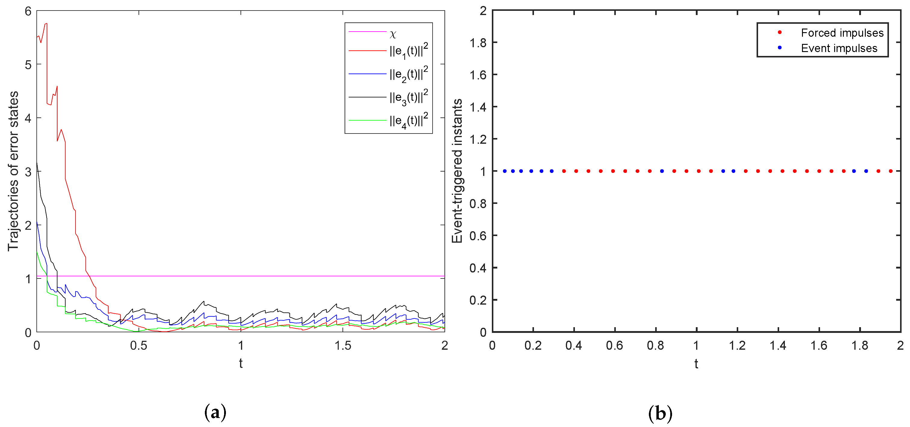
. Hence, the conditions in Theorem 1 are satisfied, and the quasi-consensus can be achieved with the error bound χ = 1.0446 . Moreover, setting l k 1.2 and υ = 1.2 , one can check that conditions in Theorem 2 are also met, and Zeno behavior can be excluded. Let λ = 1 , the trajectories of error states and event-triggered instants under ETM (9) are shown as Figure 2a,b, respectively.
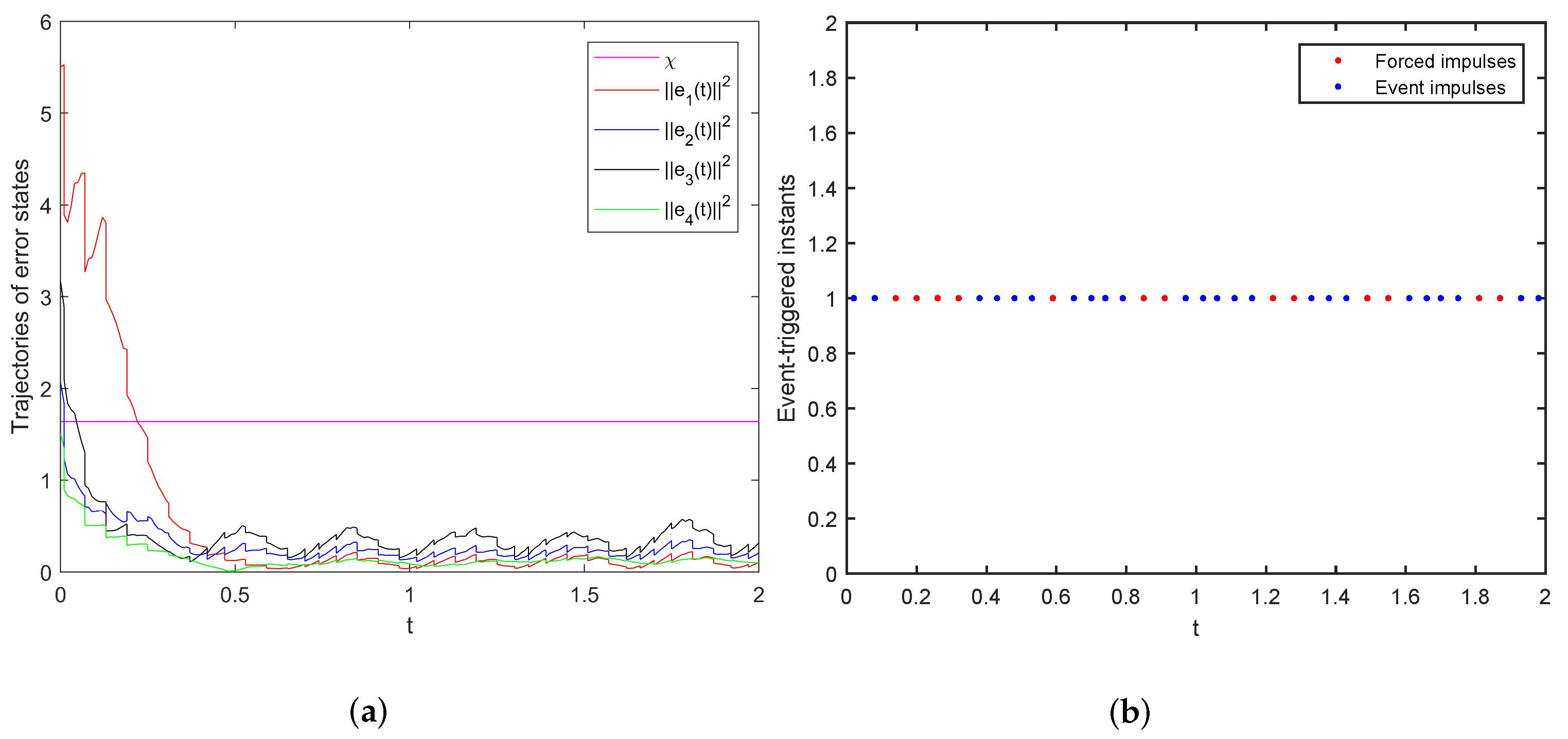
To highlight the superiority of the obtained results in this paper, the results (Theorem 2) in [31] are considered, where their ETM is designed as follows (the fixed maximum allowable event-trigger interval ρ k = ρ sup case is considered):
t k = min { t k * , t k 1 + ρ sup } , t k * = inf t > t k 1 | η ( t ) α 1 e ( t k 1 ) + λ ¯ e α 2 ( t t k 1 ) ,
where η ( t ) = e ( t ) e ( t k 1 ) , k N + and α 1 , α 2 , λ ¯ > 0 .
Neglecting the delay considered in [31], a set of feasible solutions for LMIs in (Theorem 2 in [31]) are obtained by setting ε 1 = 1 , β 1 = 2 and μ ¯ = 0.8 . Then, one has β 2 1.3934 and ρ sup < 0.0595 with β 2 = 1.4 . Choose ρ sup = 0.05 , α 1 = 0.5 , α 2 = 1 , λ ¯ = e 1.5 and K = 0.1 I 4 ; it is calculated that the error bound under (33) is χ = 1.6378 with w ˜ = 1.2 and η = 1.0623 . With the parameters above, the trajectories of error states and event-triggered instants under ETM (9) are shown as Figure 3a,b, respectively.
Compared with the performance of both ETM (9) and (33), one can find that the error bound χ is smaller, and the triggered instants are fewer under ETM (9) than those under ETM (33). Hence, less conservative results can be obtained with the ETM designed in this paper.
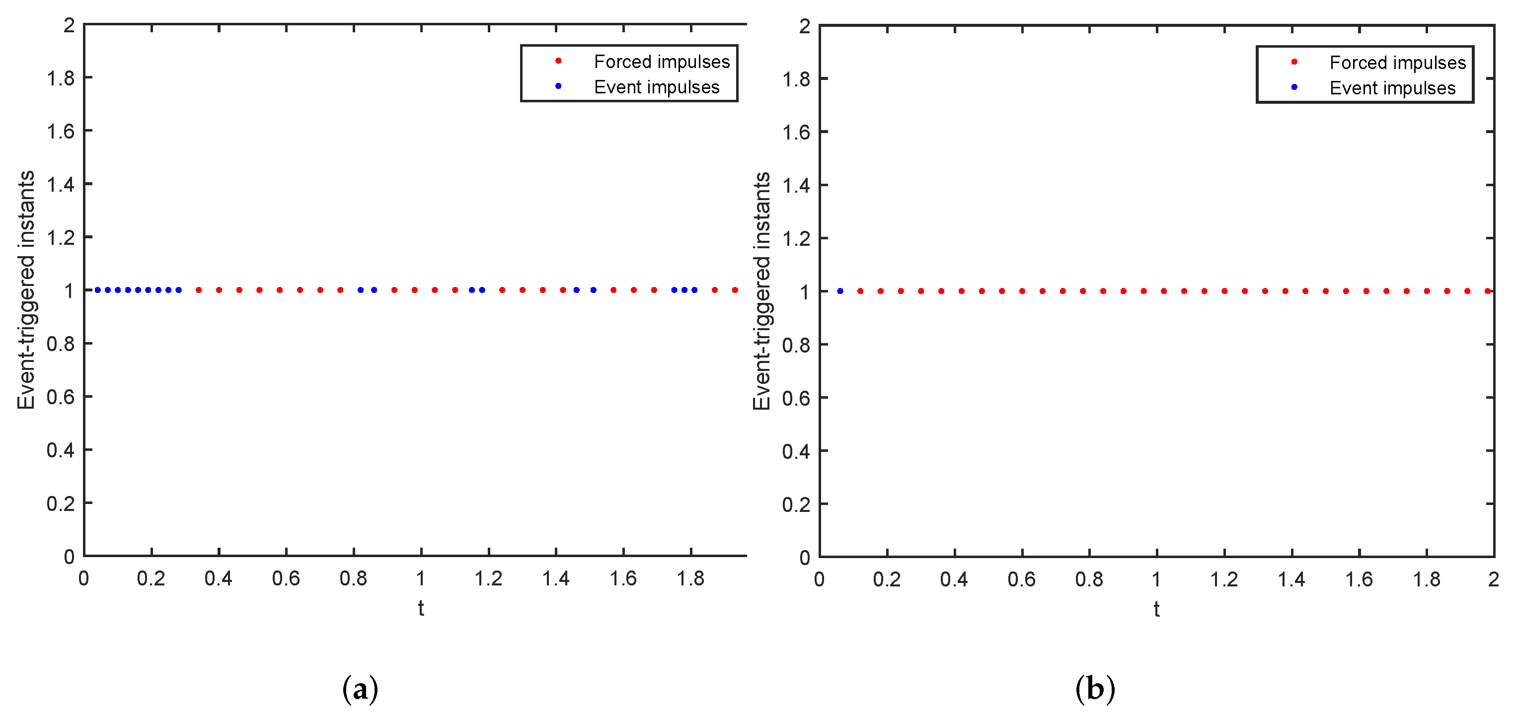
Setting λ = 2 and λ = 0.1 , the event-triggered instants of the system are shown as Figure 4a,b, respectively. By assigning different values of the parameter λ , we can obviously observe that the larger λ leads to more event-triggered instants generated by t k * .
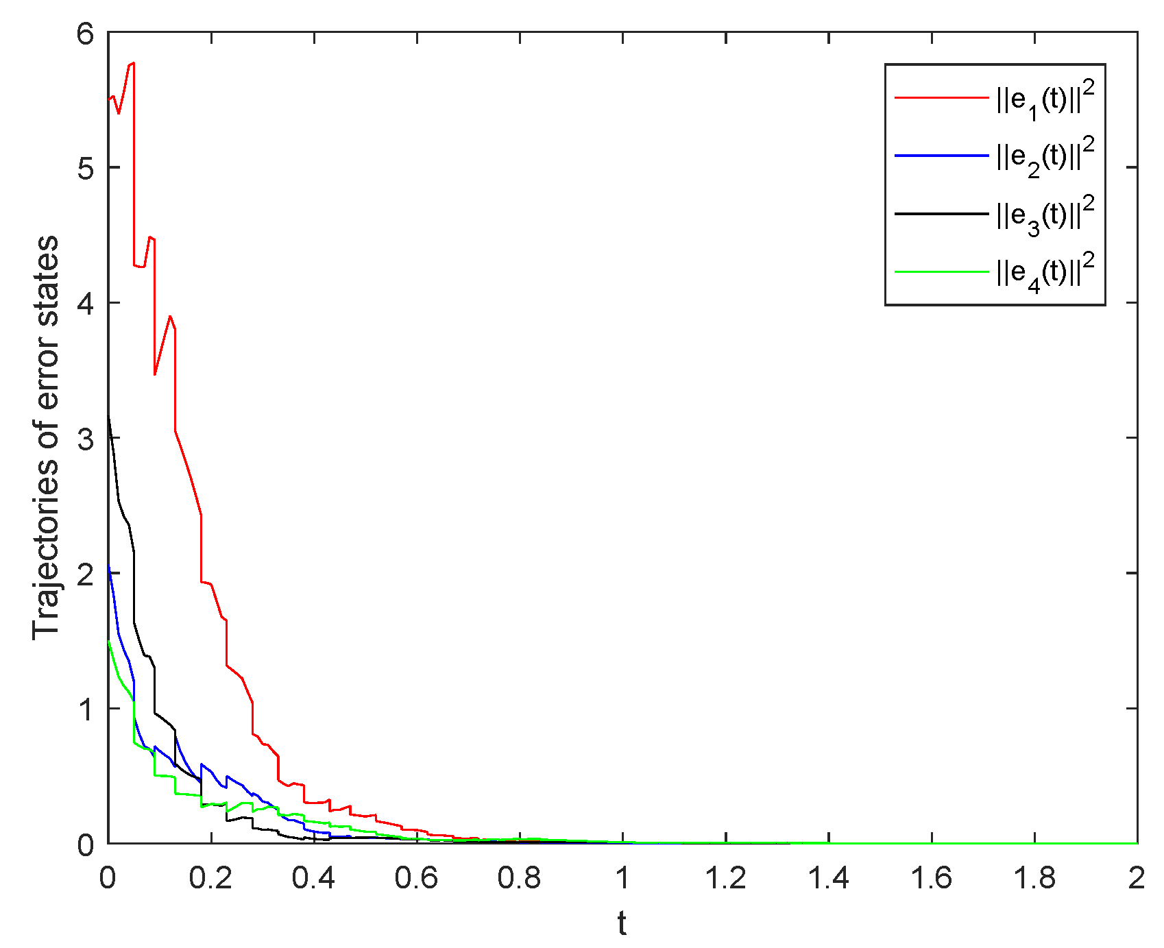
Moreover, when the external disturbances are ignored ( w i ( t ) 0 , i = 0 , 1 , 2 , 3 , 4 ), the consensus can be achieved as shown in Figure 5, i.e., the case that χ = 0 in Definition 2.

5. Conclusions

This paper investigated the quasi-consensus of nonlinear MASs with external disturbances via ETIC. The ETM designed here relies on the Lyapunov function and the compared exponential-like function with tunable parameters. To avoid Zeno behavior, Theorem 2 shows that the tunable parameters cannot be assigned arbitrarily but with some easy-to-check conditions. Meanwhile, an example verifies the obtained results. It is shown that our results are less conservative compared with the existing results. However, the considered MASs are free of time delays [37]; thus, an interesting research topic for further study is to consider time delays in the systems.

Author Contributions

Conceptualization, Z.G.; methodology, Z.G. and S.P.; software, Z.G.; validation, Z.G. and S.P.; resources, Z.G.; data curation, Z.G. and Y.H.; writing—original draft preparation, Z.G.; writing—review and editing, Z.G. and S.P. All authors have read and agreed to the published version of the manuscript.

Funding

This work was supported in part by the National Natural Science Foundation of China under Grant 61973092 and in part by the Guangdong Basic and Applied Basic Research Foundation under Grant 2019A1515012104.

Institutional Review Board Statement

Not applicable.

Informed Consent Statement

Not applicable.

Data Availability Statement

Not applicable.

Conflicts of Interest

The authors declare no conflict of interest.

References

  1. Yao, Z.; Wu, S.; Wen, Y. Formation generation for multiple unmanned vehicles using multiagent hybrid social cognitive optimization based on the internet of things. Sensors 2019, 19, 1600. [Google Scholar] [CrossRef] [PubMed] [Green Version]
  2. Mansour, A.M.; Obeidat, M.A.; Abdallah, J. A novel multiagent mechanism for managing electrical power smart grids. In Proceedings of the 2021 12th International Renewable Engineering Conference (IREC), Amman, Jordan, 14–15 April 2021; pp. 1–6. [Google Scholar]
  3. Simões, M.A.; da Silva, R.M.; Nogueira, T. A dataset schema for cooperative learning from demonstration in multi-robot systems. J. Intell. Robot. Syst. 2020, 99, 589–608. [Google Scholar] [CrossRef] [Green Version]
  4. Zheng, Y.; Ma, J.; Wang, L. Consensus of hybrid multiagent systems. IEEE Trans. Neural Netw. Learn. Syst. 2017, 29, 1359–1365. [Google Scholar] [CrossRef] [PubMed] [Green Version]
  5. Ma, L.; Wang, Z.; Han, Q.L.; Liu, Y. Consensus control of stochastic multiagent systems: A survey. Sci. China Inf. Sci. 2017, 60, 120201. [Google Scholar] [CrossRef] [Green Version]
  6. Ma, T.; Zhang, Z.; Cui, B. Variable impulsive consensus of nonlinear multiagent systems. Nonlinear Anal. Hybrid Syst. 2019, 31, 1–18. [Google Scholar] [CrossRef]
  7. Meng, M.; Xiao, G.; Li, B. Adaptive consensus for heterogeneous multiagent systems under sensor and actuator attacks. Automatica 2020, 122, 109242. [Google Scholar] [CrossRef]
  8. Hu, H.; Yu, L.; Chen, G.; Xie, G. Second-order consensus of multiagent systems with unknown but bounded disturbance. Int. J. Control. Autom. Syst. 2013, 11, 258–267. [Google Scholar] [CrossRef]
  9. Ma, L.; Wang, Z.; Yuan, Y. Consensus control for nonlinear multiagent systems subject to deception attacks. In Proceedings of the 2016 22nd International Conference on Automation and Computing (ICAC), Colchester, UK, 7–8 September 2016; pp. 21–26. [Google Scholar]
  10. Wang, Z.; Wang, Y.; Liu, Y. Global synchronization for discrete-time stochastic complex networks with randomly occurred nonlinearities and mixed time delays. IEEE Trans. Neural Netw. 2009, 21, 11–25. [Google Scholar] [CrossRef] [Green Version]
  11. Almeida, R.; Girejko, E.; Hristova, S.; Malinowska, A.B. Leader-following consensus for fractional multiagent systems. Adv. Differ. Equ. 2019, 2019, 301. [Google Scholar] [CrossRef] [Green Version]
  12. Liu, K.; Duan, P.; Duan, Z.; Cai, H.; Lü, J. Leader-following consensus of multiagent systems with switching networks and event-triggered control. IEEE Trans. Circuits Syst. I Regul. Pap. 2017, 65, 1696–1706. [Google Scholar] [CrossRef]
  13. Hu, J.; Wang, Z.; Gao, H.; Stergioulas, L.K. Robust sliding mode control for discrete stochastic systems with mixed time delays, randomly occurring uncertainties, and randomly occurring nonlinearities. IEEE Trans. Ind. Electron. 2011, 59, 3008–3015. [Google Scholar] [CrossRef] [Green Version]
  14. Hu, M.; Guo, L.; Hu, A.; Yang, Y. Leader-following consensus of linear multiagent systems with randomly occurring nonlinearities and uncertainties and stochastic disturbances. Neurocomputing 2015, 149, 884–890. [Google Scholar] [CrossRef]
  15. Xu, Y.; Peng, S.; Guo, A. Leader-following consensus of nonlinear multiagent systems with randomly occurring uncertainties and stochastic disturbances under impulsive control input. Int. J. Syst. Sci. 2017, 48, 3138–3146. [Google Scholar] [CrossRef]
  16. Ren, H.; Deng, F.; Peng, Y.; Zhang, B.; Zhang, C. Exponential consensus of non-linear stochastic multiagent systems with ROUs and RONs via impulsive pinning control. IET Control Theory Appl. 2017, 11, 225–236. [Google Scholar] [CrossRef]
  17. Zhang, Z.; Peng, S.; Chen, T. Leader-following mean square consensus of stochastic multiagent systems with ROUs and RONs under periodically variable impulse time windows. Neurocomputing 2020, 412, 276–286. [Google Scholar] [CrossRef]
  18. Wang, D.; Wang, W. Necessary and sufficient conditions for containment control of multiagent systems with time delay. Automatica 2019, 103, 418–423. [Google Scholar] [CrossRef]
  19. Deng, C.; Yang, G.H. Distributed adaptive fault-tolerant control approach to cooperative output regulation for linear multiagent systems. Automatica 2019, 103, 62–68. [Google Scholar] [CrossRef]
  20. Zhou, Y.J.; Jiang, G.P.; Xu, F.Y.; Chen, Q.Y. Distributed finite time consensus of second-order multiagent systems via pinning control (August 2018). IEEE Access 2018, 6, 45617–45624. [Google Scholar] [CrossRef]
  21. Li, X.; Song, S. Stabilization of delay systems: Delay-dependent impulsive control. IEEE Trans. Autom. Control 2016, 62, 406–411. [Google Scholar] [CrossRef]
  22. Zhang, X.; Lv, X.; Li, X. Sampled-data-based lag synchronization of chaotic delayed neural networks with impulsive control. Nonlinear Dyn. 2017, 90, 2199–2207. [Google Scholar] [CrossRef]
  23. Yang, S.; Liu, Y.; Xiao, Y.; Wu, T. Consensus of delayed multiagent dynamical systems with stochastic perturbation via dual-stage impulsive approach. Nonlinear Dyn. 2019, 95, 893–903. [Google Scholar] [CrossRef]
  24. Tabuada, P. Event-triggered real-time scheduling of stabilizing control tasks. IEEE Trans. Autom. Control 2007, 52, 1680–1685. [Google Scholar] [CrossRef] [Green Version]
  25. Hu, W.; Liu, L.; Feng, G. Consensus of linear multiagent systems by distributed event-triggered strategy. IEEE Trans. Cybern. 2015, 46, 148–157. [Google Scholar] [CrossRef] [PubMed]
  26. Dolk, V.; Borgers, D.P.; Heemels, W. Output-based and decentralized dynamic event-triggered control with guaranteed L2-gain performance and zeno-freeness. IEEE Trans. Autom. Control 2016, 62, 34–49. [Google Scholar] [CrossRef]
  27. Deng, C.; Er, M.J.; Yang, G.H.; Wang, N. Event-triggered consensus of linear multiagent systems with time-varying communication delays. IEEE Trans. Cybern. 2019, 50, 2916–2925. [Google Scholar] [CrossRef]
  28. Tan, X.; Cao, J.; Li, X. Consensus of leader-following multiagent systems: A distributed event-triggered impulsive control strategy. IEEE Trans. Cybern. 2018, 49, 792–801. [Google Scholar] [CrossRef]
  29. Peng, D.; Li, X. Leader-following synchronization of complex dynamic networks via event-triggered impulsive control. Neurocomputing 2020, 412, 1–10. [Google Scholar] [CrossRef]
  30. Chen, J.; Chen, B.; Zeng, Z. Synchronization in multiple neural networks with delay and disconnected switching topology via event-triggered impulsive control strategy. IEEE Trans. Ind. Electron. 2020, 68, 2491–2500. [Google Scholar] [CrossRef]
  31. Xie, X.; Wei, T.; Li, X. Hybrid event-triggered approach for quasi-consensus of uncertain multiagent systems with impulsive protocols. IEEE Trans. Circuits Syst. I Regul. Pap. 2022, 69, 872–883. [Google Scholar] [CrossRef]
  32. Chen, T.; Peng, S.; Zhang, Z. Finite-time consensus of leader-following non-linear multiagent systems via event-triggered impulsive control. IET Control Theory Appl. 2021, 15, 926–936. [Google Scholar] [CrossRef]
  33. Zhang, Z.; Peng, S.; Liu, D.; Wang, Y.; Chen, T. Leader-following mean-square consensus of stochastic multiagent systems with ROUs and RONs via distributed event-triggered impulsive control. IEEE Trans. Cybern. 2020, 52, 1836–1849. [Google Scholar] [CrossRef] [PubMed]
  34. Liu, J.; Zhang, Y.; Yu, Y.; Sun, C. Fixed-time leader–follower consensus of networked nonlinear systems via event/self-triggered control. IEEE Trans. Neural Netw. Learn. Syst. 2020, 31, 5029–5037. [Google Scholar] [CrossRef] [PubMed]
  35. Guan, Z.H.; Hu, B.; Chi, M.; He, D.X.; Cheng, X.M. Guaranteed performance consensus in second-order multiagent systems with hybrid impulsive control. Automatica 2014, 50, 2415–2418. [Google Scholar] [CrossRef]
  36. Li, X.; Li, P. Input-to-state stability of nonlinear systems: Event-triggered impulsive control. IEEE Trans. Autom. Control 2021, 67, 1460–1465. [Google Scholar] [CrossRef]
  37. Ali, B.; Abbas, M. Existence and stability of fixed point set of Suzuki-type contractive multivalued operators in b-metric spaces with applications in delay differential equations. J. Fixed Point Theory Appl. 2017, 19, 2327–2347. [Google Scholar] [CrossRef]
Figure 1. Communication topology of the system.
Applsci 12 07580 g001
Figure 2. Trajectories of error states and event-triggered instants under ETM (9). (a) Trajectories of error states; (b) event-triggered instants.
Applsci 12 07580 g002
Figure 3. Trajectories of error states and event-triggered instants under ETM (33). (a) Trajectories of error states; (b) event-triggered instants.
Applsci 12 07580 g003
Figure 4. Event-triggered instants with different λ under ETM (9). (a) Event-triggered instants with λ = 2 ; (b) Event-triggered instants with λ = 0.1 .
Applsci 12 07580 g004
Figure 5. Trajectories of error states without external disturbances under ETM (9).
Applsci 12 07580 g005
Publisher’s Note: MDPI stays neutral with regard to jurisdictional claims in published maps and institutional affiliations.

