
Non-Invasive Evaluation of Polymeric Protective Coatings for Metal Surfaces of Cultural Heritage Objects: Comparison of Optical and Electromagnetic Methods

 ,
,  ,
, 


Abstract
:Featured Application
Abstract
1. Introduction
2. Materials and Methods
2.1. Sample Preparation
2.2. Spectral-Domain Optical Coherence Tomography (SD-OCT)
2.3. Confocal Raman Microspectroscopy (CRM)
2.4. Eddy Current (EC)
3. Results
3.1. Spectral-Domain Optical Coherence Tomography (SD-OCT)
3.2. Benchtop Instrumentation: Confocal Raman Microspectroscopy (CRM)
4. Discussion: Optical vs. Electromagnetic Methods
5. Conclusions
Author Contributions
Funding
Institutional Review Board Statement
Informed Consent Statement
Data Availability Statement
Conflicts of Interest
Appendix A

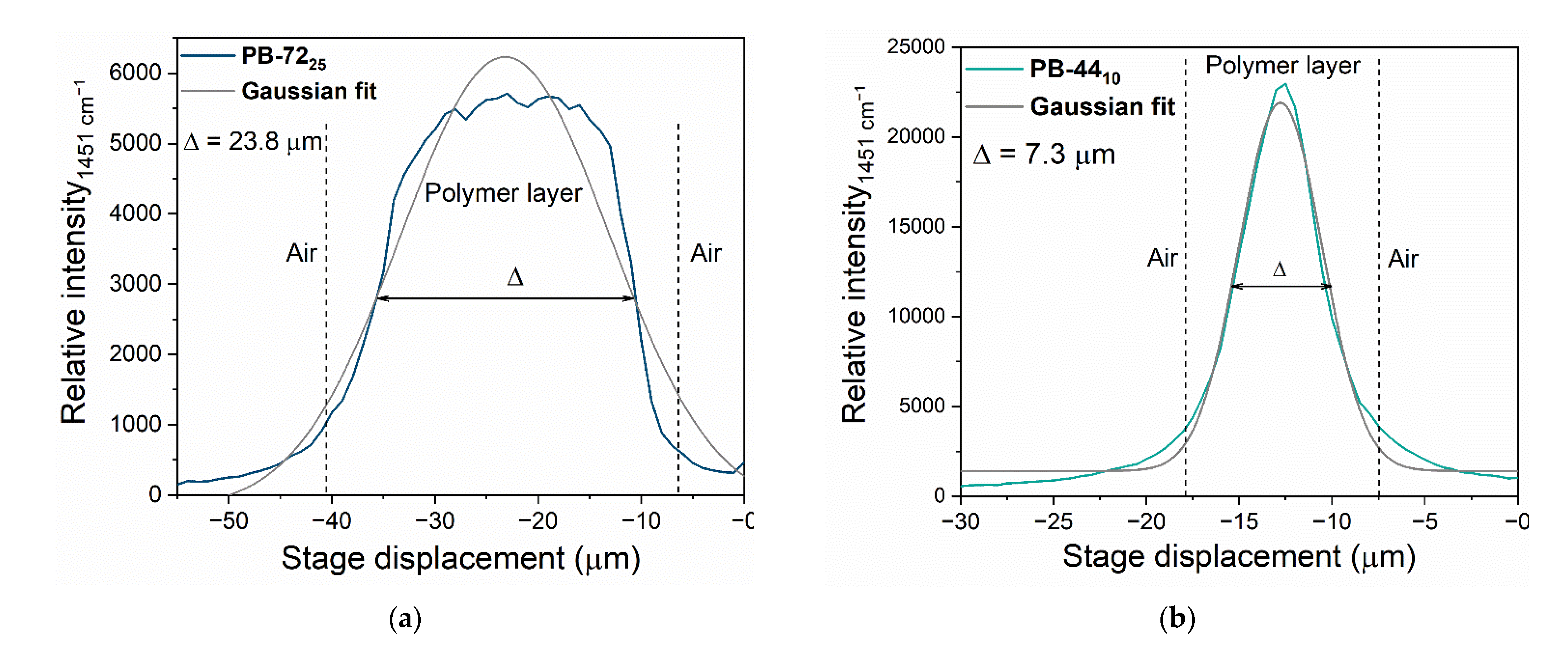
| Sample | Band (cm−1) | Δ (μm) | Std. dev. (μm) | Difference (μm) |
|---|---|---|---|---|
| PB-7230 | 1725 | 42.32 | 3.44 | 0.54 |
| 1451 | 41.78 | 3.22 | ||
| PB-4425 | 1451 | 18.69 | 1.16 | 0.05 |
| 812 | 18.64 | 1.23 | ||
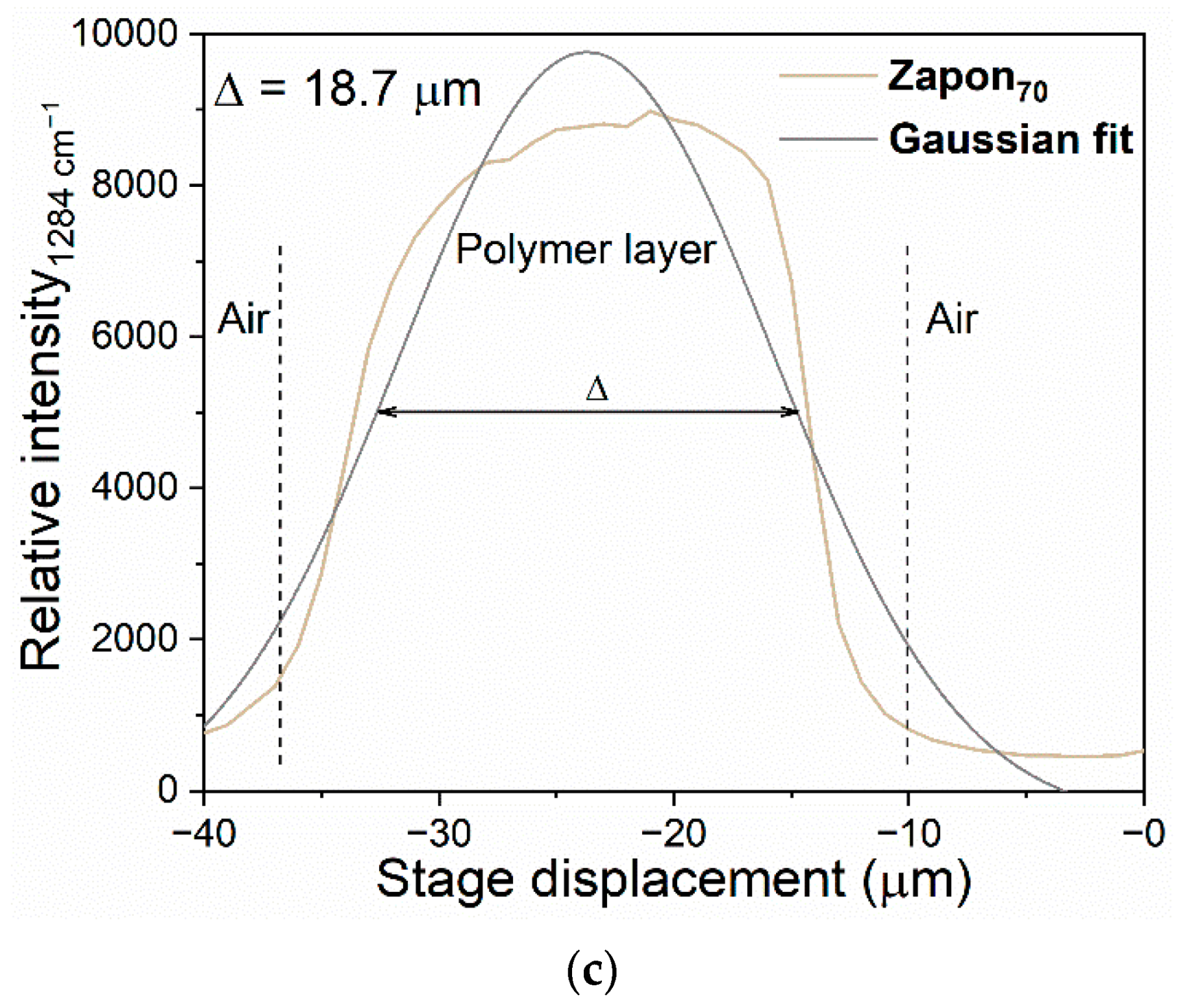
| Zapon70 | 1284 | 18.17 | 0.49 | 0.19 |
| 854 | 17.98 | 0.68 |
References
- Fayomi, O.S.I.; Akande, I.G.; Odigie, S. Economic Impact of Corrosion in Oil Sectors and Prevention: An Overview. J. Phys. Conf. Ser. 2019, 1378, 022037. [Google Scholar] [CrossRef]
- Cano, E.; Lafuente, D.; Bastidas, D.M. Use of EIS for the evaluation of the protective properties of coatings for metallic cultural heritage: A review. J. Solid State Electrochem. 2010, 14, 381–391. [Google Scholar] [CrossRef] [Green Version]
- Scott, D.A. Copper and Bronze in Art. Corrosion, Colorants, Conservation; The Getty Conservation Institute: Los Angeles, CA, USA, 2002; ISBN 0-89236-638-9. [Google Scholar]
- Cano, E.; Bastidas, D.M.; Argyropoulos, V.; Fajardo, S.; Siatou, A.; Bastidas, J.M.; Degrigny, C. Electrochemical characterization of organic coatings for protection of historic steel artefacts. J. Solid State Electrochem. 2010, 14, 453–463. [Google Scholar] [CrossRef] [Green Version]
- Kovács, R.L.; Daróczi, L.; Barkóczy, P.; Baradács, E.; Bakonyi, E.; Kovács, S.; Erdélyi, Z. Water vapor transmission properties of acrylic organic coatings. J. Coat. Technol. Res. 2021, 18, 523–534. [Google Scholar] [CrossRef]
- Favaro, M.; Mendichi, R.; Ossola, F.; Russo, U.; Simon, S.; Tomasin, P.; Vigato, P.A. Evaluation of polymers for conservation treatments of outdoor exposed stone monuments. Part I: Photo-oxidative weathering. Polym. Degrad. Stab. 2006, 91, 3083–3096. [Google Scholar] [CrossRef]
- Artesani, A.; Di Turo, F.; Zucchelli, M.; Traviglia, A. Recent Advances in Protective Coatings for Cultural Heritage—An Overview. Coatings 2020, 10, 217. [Google Scholar] [CrossRef] [Green Version]
- Letardi, P. Testing New Coatings for Outdoor Bronze Monuments: A Methodological Overview. Coatings 2021, 11, 131. [Google Scholar] [CrossRef]
- England, A.; Hosbein, K.; Price, C.; Wylder, M.; Miller, K.; Clare, T. Assessing the Protective Quality of Wax Coatings on Bronze Sculptures Using Hydrogel Patches in Impedance Measurements. Coatings 2016, 6, 45. [Google Scholar] [CrossRef] [Green Version]
- Agnoletti, S.; Bruni, T.; Cagnini, A.; Galeotti, M.; Porcinai, S. Le applicazioni della tecnica delle correnti indotte (Eddy-Current) per la conservazione e lo studio di manufatti metallici di valore storico-artistico. OPD Restauro 2016, 28, 162–173. [Google Scholar]
- Sousa, J.B.; Ventura, J.O.; Pereira, A. Noncontact techniques. In Transport Phenomena in Micro- and Nanoscale Functional Materials and Devices; Elsevier: Amsterdam, The Netherlands, 2021; pp. 273–307. ISBN 978-0-323-46097-2. [Google Scholar]
- García-Martín, J.; Gómez-Gil, J.; Vázquez-Sánchez, E. Non-Destructive Techniques Based on Eddy Current Testing. Sensors 2011, 11, 2525–2565. [Google Scholar] [CrossRef] [PubMed] [Green Version]
- Meng, X.; Lu, M.; Yin, W.; Bennecer, A.; Kirk, K.J. Evaluation of Coating Thickness Using Lift-Off Insensitivity of Eddy Current Sensor. Sensors 2021, 21, 419. [Google Scholar] [CrossRef] [PubMed]
- Lenz, M.; Mazzon, C.; Dillmann, C.; Gerhardt, N.; Welp, H.; Prange, M.; Hofmann, M. Spectral Domain Optical Coherence Tomography for Non-Destructive Testing of Protection Coatings on Metal Substrates. Appl. Sci. 2017, 7, 364. [Google Scholar] [CrossRef] [Green Version]
- Porcinai, S.; Ferretti, M. X-ray fluorescence-based methods to measure the thickness of protective organic coatings on ancient silver artefacts. Spectrochim. Acta Part B At. Spectrosc. 2018, 149, 184–189. [Google Scholar] [CrossRef]
- Porcinai, S.; Heginbotham, A. Thickness mapping of organic layers applied on sterling silver by means of X-ray fluorescence scanning. Spectrochim. Acta Part B At. Spectrosc. 2021, 180, 106158. [Google Scholar] [CrossRef]
- Catelli, E.; Sciutto, G.; Prati, S.; Jia, Y.; Mazzeo, R. Characterization of outdoor bronze monument patinas: The potentialities of near-infrared spectroscopic analysis. Environ. Sci. Pollut. Res. 2018, 25, 24379–24393. [Google Scholar] [CrossRef] [PubMed]
- Crawford, M.K.; Fair, L.; Rovito, K.; Polidori, T.; Grayburn, R. Thickness Measurements of Clear Coatings on Silver Objects using Fiber Optic Reflectance Spectroscopy. J. Am. Inst. Conserv. 2021, 61, 71–84. [Google Scholar] [CrossRef]
- Barra, V.; Daffara, C.; Porcinai, S.; Galeotti, M. Application of coatings on silver studied with punctual and imaging techniques: From specimens to real cases. IOP Conf. Ser. Mater. Sci. Eng. 2018, 364, 012059. [Google Scholar] [CrossRef]
- Dal Fovo, A.; Mattana, S.; Chaban, A.; Quintero Balbas, D.; Lagarto, J.L.; Striova, J.; Cicchi, R.; Fontana, R. Fluorescence Lifetime Phasor Analysis and Raman Spectroscopy of Pigmented Organic Binders and Coatings Used in Artworks. Appl. Sci. 2021, 12, 179. [Google Scholar] [CrossRef]
- Boyatzis, S.C.; Douvas, A.M.; Argyropoulos, V.; Siatou, A.; Vlachopoulou, M. Characterization of a Water-Dispersible Metal Protective Coating with Fourier Transform Infrared Spectroscopy, Modulated Differential Scanning Calorimetry, and Ellipsometry. Appl. Spectrosc. 2012, 66, 580–590. [Google Scholar] [CrossRef]
- Antoniuk, P.; Strąkowski, M.R.; Pluciński, J.; Kosmowski, B.B. Non-destructive inspection of anti-corrosion protective coatings using Optical Coherent Tomography. Metrol. Meas. Syst. 2012, XIX, 365–372. [Google Scholar] [CrossRef] [Green Version]
- Tomba, J.P.; de la Paz Miguel, M.; Perez, C.J. Correction of optical distortions in dry depth profiling with confocal Raman microspectroscopy: Distortion correction in dry depth profiling with confocal Raman microspectroscopy. J. Raman Spectrosc. 2011, 42, 1330–1334. [Google Scholar] [CrossRef]
- Lorenzetti, G.; Striova, J.; Zoppi, A.; Castellucci, E.M. Confocal Raman microscopy for in depth analysis in the field of cultural heritage. J. Mol. Struct. 2011, 993, 97–103. [Google Scholar] [CrossRef]
- Everall, N.J. Confocal Raman microscopy: Common errors and artefacts. Analyst 2010, 135, 2512–2522. [Google Scholar] [CrossRef] [PubMed]
- Schmidt, U.; Ibach, W.; Mueller, J.; Hollricher, O. The Confocal Raman AFM: A Powerful Tool for the Characterization of Surface Coatings. In Optical Measurement Systems for Industrial Inspection V; Osten, W., Gorecki, C., Novak, E.L., Eds.; Proc. SPIE: Munich, Germany, 2007; Volume 66160E, pp. 119–124. [Google Scholar] [CrossRef]
- Ntelia, E.; Karapanagiotis, I. Superhydrophobic Paraloid B72. Prog. Org. Coat. 2020, 139, 105224. [Google Scholar] [CrossRef]
- Tennent, N.H.; Townsend, J.H. The significance of the refractive index of adhesives for glass repair. Stud. Conserv. 1984, 29, 205–212. [Google Scholar] [CrossRef]
- Down, J.L.; MacDonald, M.A.; Tétreault, J.; Williams, A.S. Adhesive Testing at the Canadian Conservation Institute: An Evaluation of Selected Poly(Vinyl Acetate) and Acrylic Adhesives. Stud. Conserv. 1996, 41, 19–44. [Google Scholar]
- Vinçotte, A.; Beauvoit, E.; Boyard, N.; Guilminot, E. Effect of solvent on PARALOID® B72 and B44 acrylic resins used as adhesives in conservation. Herit. Sci. 2019, 7, 42. [Google Scholar] [CrossRef]
- Argyropoulos, V.; Giannoulaki, M.; Michalakakos, G.P.; Siatou, A. A Survey of the Types of Corrosion Inhibitors and Protective Coatings Used for the Conservation of Metal Objects from Museum Collections in the Mediterranean Basin; Department of Conservation of Antiquities and Works of Art & T.E.I. of Athens: Cairo, Egypt, 2007; pp. 1–5. [Google Scholar]
- Holben Ellis, M. The Shifting Function of Artists’ Fixatives. J. Am. Inst. Conserv. 1996, 35, 239–254. [Google Scholar] [CrossRef]
- Conn, G.K.T.; Eaton, G.K. On Polarization by Transmission with Particular Reference to Selenium Films in the Infrared. J. Opt. Soc. Am. 1954, 44, 553–557. [Google Scholar] [CrossRef]
- Chapman, S.; Mason, D. Literature Review: The use of Paraloid B-72 as a surface consolidant for stained glass. J. Am. Inst. Conserv. 2003, 42, 381–392. [Google Scholar] [CrossRef]
- Paraloid B-44—CAMEO. Available online: https://cameo.mfa.org/wiki/Paraloid_B-44 (accessed on 14 June 2022).
- Ohlídalová, M.; Kučerová, I.; Novotná, M. Identification of acrylic consolidants in wood by Raman spectroscopy. J. Raman Spectrosc. 2006, 37, 1179–1185. [Google Scholar] [CrossRef]
- Neves, A.; Angelin, E.M.; Roldão, É.; Melo, M.J. New insights into the degradation mechanism of cellulose nitrate in cinematographic films by Raman microscopy. J. Raman Spectrosc. 2019, 50, 202–212. [Google Scholar] [CrossRef]
- Tfayli, A.; Piot, O.; Manfait, M. Confocal Raman microspectroscopy on excised human skin: Uncertainties in depth profiling and mathematical correction applied to dermatological drug permeation. J. Biophotonics 2008, 1, 140–153. [Google Scholar] [CrossRef] [PubMed]
- Everall, N.J. Confocal Raman Microscopy: Why the Depth Resolution and Spatial Accuracy Can Be Much Worse Than You Think. Appl. Spectrosc. 2000, 54, 1515–1520. [Google Scholar] [CrossRef]


| Polymer | Chemical Composition | Refractive Index | Tg (° C) | Sample Code | Concentration in Butyl Acetate (W %) |
|---|---|---|---|---|---|
| Paraloid® B-72 | methyl acrylate/ethyl methacrylate copolymer | 1.49 [34] | 40 | PB-7230 | 30 |
| PB-7225 | 25 | ||||
| PB-7210 | 10 | ||||
| Paraloid® B-44 | methyl methacrylate/ethyl acrylate copolymer | 1.48 [35] | 60 | PB-4425 | 25 |
| PB-4410 | 10 | ||||
| PB-445 | 5 | ||||
| Zapon® | cellulose nitrate (Lacquer 30% v) | 1.54 [28] | 100 | Zapon70 | 70 (poly. conc. = ~21% v) |
| Zapon40 | 40 (poly. conc. = ~12% v) | ||||
| Zapon20 | 20 (poly. conc. = ~6% v) |
| Sample | Thickness Measurement (μm) | Mean (μm) | Std. dev. (μm) | |||||||||||
|---|---|---|---|---|---|---|---|---|---|---|---|---|---|---|
| 1 | 2 | 3 | 4 | 5 | 6 | 7 | 8 | 9 | 10 | 11 | 12 | |||
| PB-7230 | 50.8 | 45.1 | 38.0 | 29.2 | 25.5 | 25.7 | 24.0 | 25.1 | 34.0 | 41.4 | 45.5 | 56.3 | 36.7 | 12.7 |
| PB-7225 | 34.3 | 32.9 | 29.9 | 25.4 | 23.7 | 21.3 | 20.9 | 19.1 | 20.1 | 31.5 | 45.0 | 36.7 | 28.4 | 9.3 |
| PB-7210 | 21.3 | 20.3 | 13.0 | 11.1 | 11.0 | 12.1 | 12.9 | 12.4 | 11.3 | 17.4 | 18.6 | 20.5 | 15.2 | 5.6 |
| PB-4425 | 34.3 | 34.8 | 30.7 | 28.4 | 22.0 | 20.5 | 18.5 | 18.9 | 23.7 | 24.8 | 45.8 | 42.4 | 28.7 | 10.0 |
| PB-4410 | 22.5 | 17.6 | 14.0 | 12.4 | 12.1 | 12.0 | 18.9 | 14.4 | 16.3 | 16.2 | 11.3 | 15.4 | 15.3 | 4.2 |
| PB-445 | 7.3 | 7.0 | 7.4 | 8.4 | 8.4 | 8.3 | 7.4 | 9.6 | 8.4 | 8.3 | 8.4 | 6.9 | 8.0 | 1.4 |
| Zapon70 | 7.9 | 8.0 | 6.9 | 7.1 | 6.8 | 7.0 | 9.3 | 6.9 | 7.0 | 6.7 | 7.1 | 7.0 | 18.8 | 5.0 |
| Zapon40 | 13.7 | 12.9 | 12.9 | 13.0 | 12.8 | 11.6 | 13.1 | 11.6 | 14.1 | 14.9 | 14.0 | 16.5 | 13.4 | 3.4 |
| Zapon20 | 7.9 | 8.0 | 6.9 | 7.1 | 6.8 | 7.0 | 9.3 | 6.9 | 7.0 | 6.7 | 7.1 | 7.0 | 7.3 | 1.1 |
| Sample | Δ (μm) | Std. dev. (μm) | (μm) | Std. dev. (μm) | hz |
|---|---|---|---|---|---|
| PB-7230 | 41.8 | 3.2 | 62.3 | 4.8 | 10.6 |
| PB-7225 | 24.2 | 0.5 | 36.1 | 0.8 | 8.0 |
| PB-7210 | 5.5 | 1.0 | 8.3 | 0.0 | 3.8 |
| PB-4425 | 18.7 | 1.2 | 27.7 | 1.7 | 7.0 |
| PB-4410 | 8.3 | 1.5 | 12.3 | 2.3 | 4.7 |
| PB-445 | 5.6 | 0.8 | 8.2 | 1.1 | 3.8 |
| Zapon70 | 18.2 | 0.5 | 28.1 | 0.8 | 7.1 |
| Zapon40 | 6.7 | 0.6 | 9.5 | 0.6 | 4.1 |
| Zapon20 | 3.5 | 0.3 | 5.5 | 0.3 | 3.1 |
| Sample | OCT (μm) Min./Max. | OCT Mean (μm) | Std. dev. (μm) | (μm) Min./Max. | Mean (μm) | Std. dev. (μm) | Eddy Current ⌀5 mm (μm) | Std. dev. (μm) |
|---|---|---|---|---|---|---|---|---|
| PB-7230 | 21.3/60.3 | 36.7 | 12.7 | 57.9/67.4 | 62.3 | 4.8 | 43 | 2 |
| PB-7225 | 17.7/50.1 | 28.4 | 9.3 | 23.8/36.6 | 36.1 | 0.8 | 32 | 2 |
| PB-7210 | 8.9/32.8 | 15.2 | 5.6 | 6.7/9.7 | 8.2 | 1.5 | 12 | 1 |
| PB-4425 | 17.7/50.0 | 28.7 | 10.0 | 25.8/29.2 | 27.7 | 1.7 | 30 | 1 |
| PB-4410 | 7.7/25.3 | 15.3 | 4.2 | 10.8/14.9 | 12.3 | 2.3 | 10 | 1 |
| PB-445 | 6.6/11.1 | 8.0 | 1.4 | 7.2/9.5 | 8.2 | 1.1 | 6 | 1 |
| Zapon70 | 9.8/28.4 | 18.8 | 5.0 | 27.5/29.0 | 28.1 | 0.8 | 20 | 1 |
| Zapon40 | 7.4/21.2 | 13.4 | 3.4 | 9.0/10.2 | 9.5 | 0.6 | 10 | 1 |
| Zapon20 | 6.5/10.6 | 7.3 | 1.1 | 5.1/5.8 | 5.5 | 0.3 | 4 | 1 |
| Technique | Portable | Area Investigated 1 | Data Correction | Contactless | Measure Time | Corrosion Interference |
|---|---|---|---|---|---|---|
| OCT | Yes | Smallest area: 13 μm2 | Yes | Yes | Relatively fast | No |
| CRM | No | Smallest area: ~1.77 μm2 (⌀1.5 μm) | Yes | Yes | Slow | No |
| EC | Yes | 19.63 mm2 (⌀5 mm) | No | No | Fast | Yes |
Publisher’s Note: MDPI stays neutral with regard to jurisdictional claims in published maps and institutional affiliations. |
© 2022 by the authors. Licensee MDPI, Basel, Switzerland. This article is an open access article distributed under the terms and conditions of the Creative Commons Attribution (CC BY) license (https://creativecommons.org/licenses/by/4.0/).
Share and Cite
Quintero Balbas, D.; Dal Fovo, A.; Porcu, D.; Chaban, A.; Porcinai, S.; Fontana, R.; Striova, J. Non-Invasive Evaluation of Polymeric Protective Coatings for Metal Surfaces of Cultural Heritage Objects: Comparison of Optical and Electromagnetic Methods. Appl. Sci. 2022, 12, 7532. https://doi.org/10.3390/app12157532
Quintero Balbas D, Dal Fovo A, Porcu D, Chaban A, Porcinai S, Fontana R, Striova J. Non-Invasive Evaluation of Polymeric Protective Coatings for Metal Surfaces of Cultural Heritage Objects: Comparison of Optical and Electromagnetic Methods. Applied Sciences. 2022; 12(15):7532. https://doi.org/10.3390/app12157532
Chicago/Turabian StyleQuintero Balbas, Diego, Alice Dal Fovo, Daniela Porcu, Antonina Chaban, Simone Porcinai, Raffaella Fontana, and Jana Striova. 2022. "Non-Invasive Evaluation of Polymeric Protective Coatings for Metal Surfaces of Cultural Heritage Objects: Comparison of Optical and Electromagnetic Methods" Applied Sciences 12, no. 15: 7532. https://doi.org/10.3390/app12157532
APA StyleQuintero Balbas, D., Dal Fovo, A., Porcu, D., Chaban, A., Porcinai, S., Fontana, R., & Striova, J. (2022). Non-Invasive Evaluation of Polymeric Protective Coatings for Metal Surfaces of Cultural Heritage Objects: Comparison of Optical and Electromagnetic Methods. Applied Sciences, 12(15), 7532. https://doi.org/10.3390/app12157532