
Hidden Dangerous Object Recognition in Terahertz Images Using Deep Learning Methods

 , ,
, ,
Abstract
:1. Introduction
2. Related Work
2.1. Terahertz Image Acquisition & Image Processing
Dataset Description
2.2. Terahertz Image Detection
- 1.
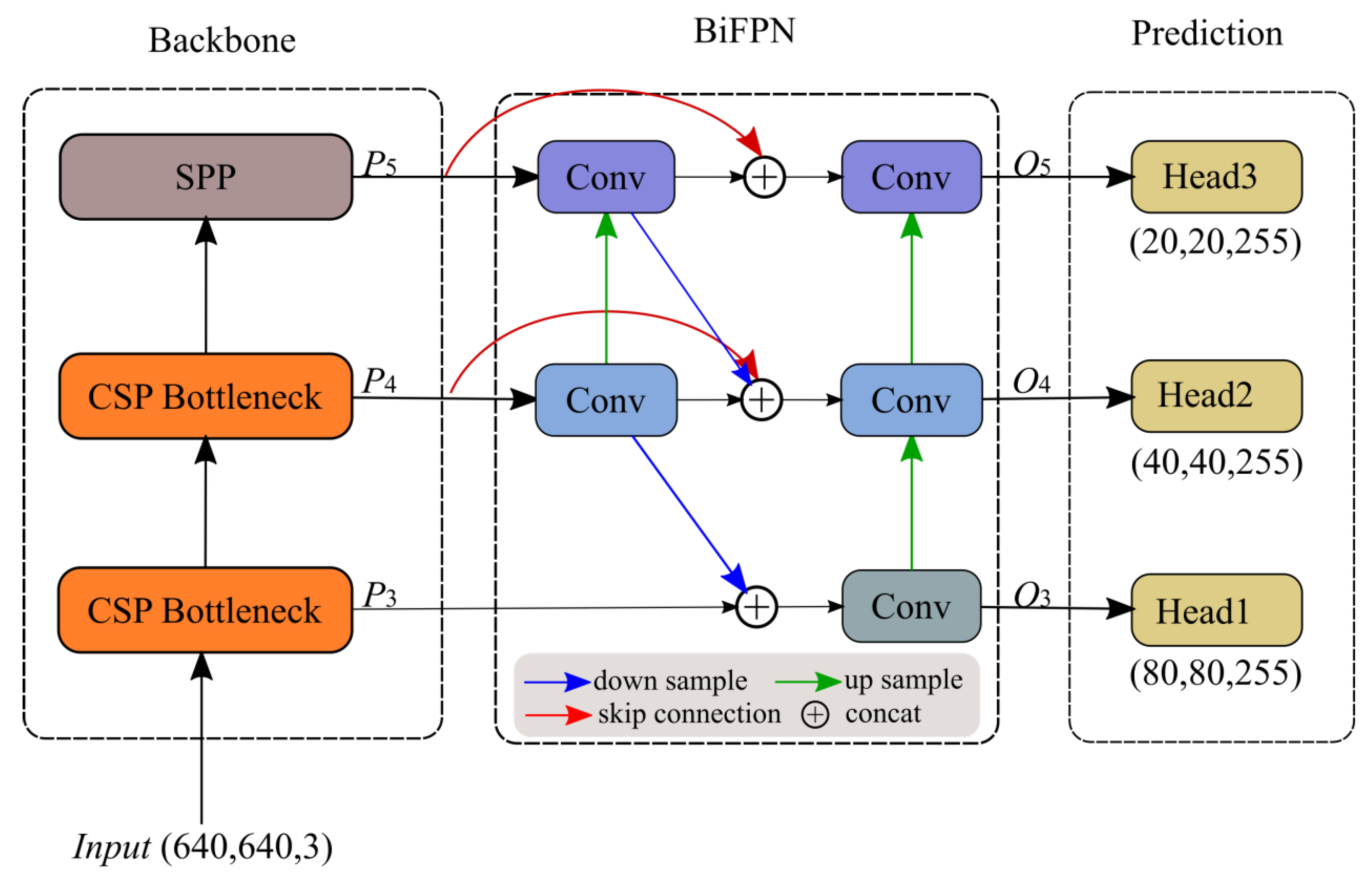
- Improving low resolution using BiFPN at the neck of YOLOv5 of the deep learning model.
- 2.
- Transfer learning is done using the fine-tuning process to the pre-training weight of the backbone for migration learning in our model.
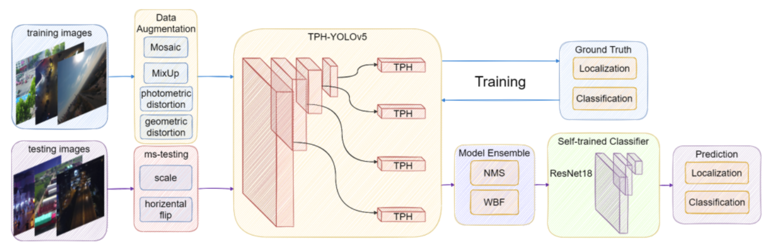
3. Proposed Model
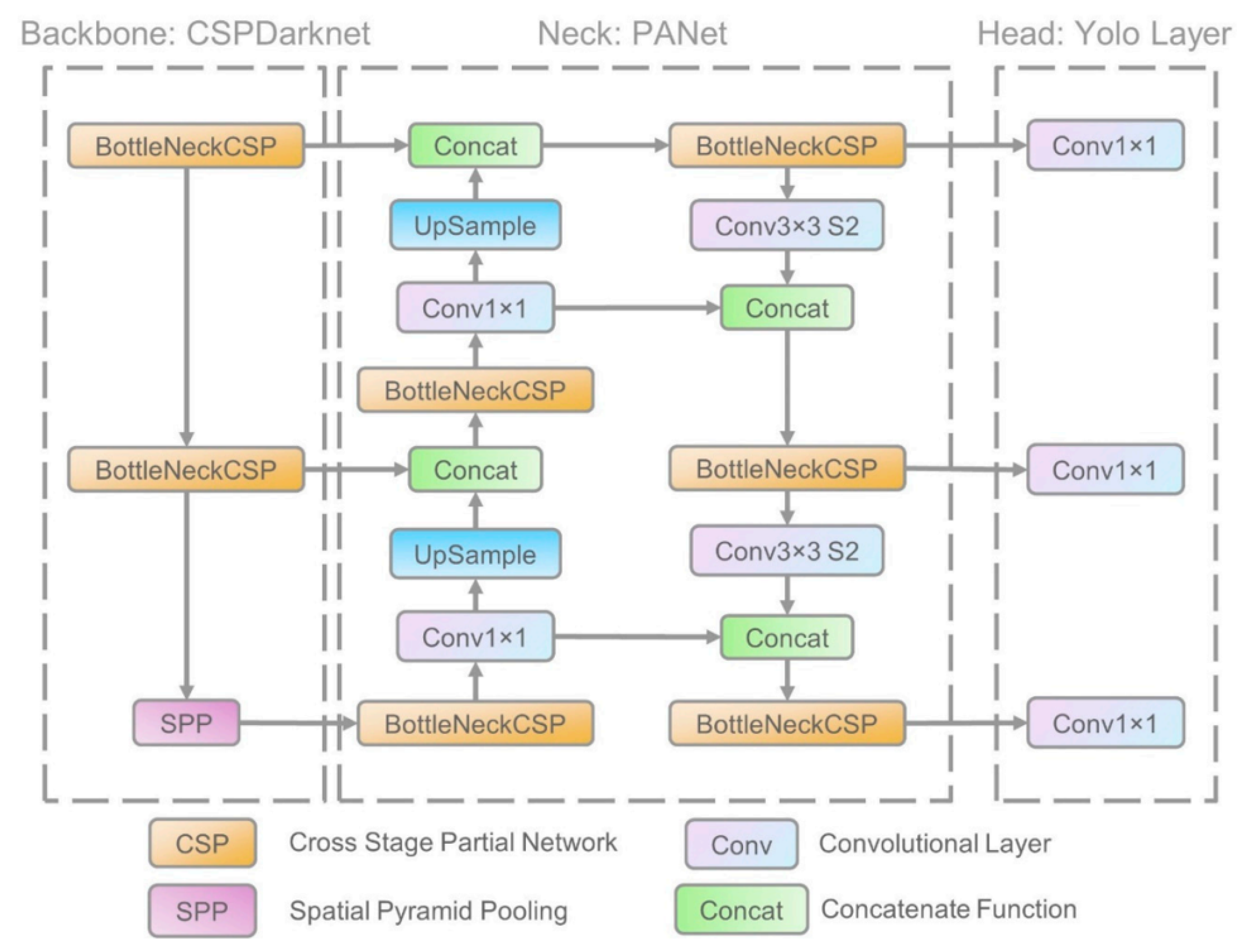
3.1. Model Backbone
3.2. Model Neck
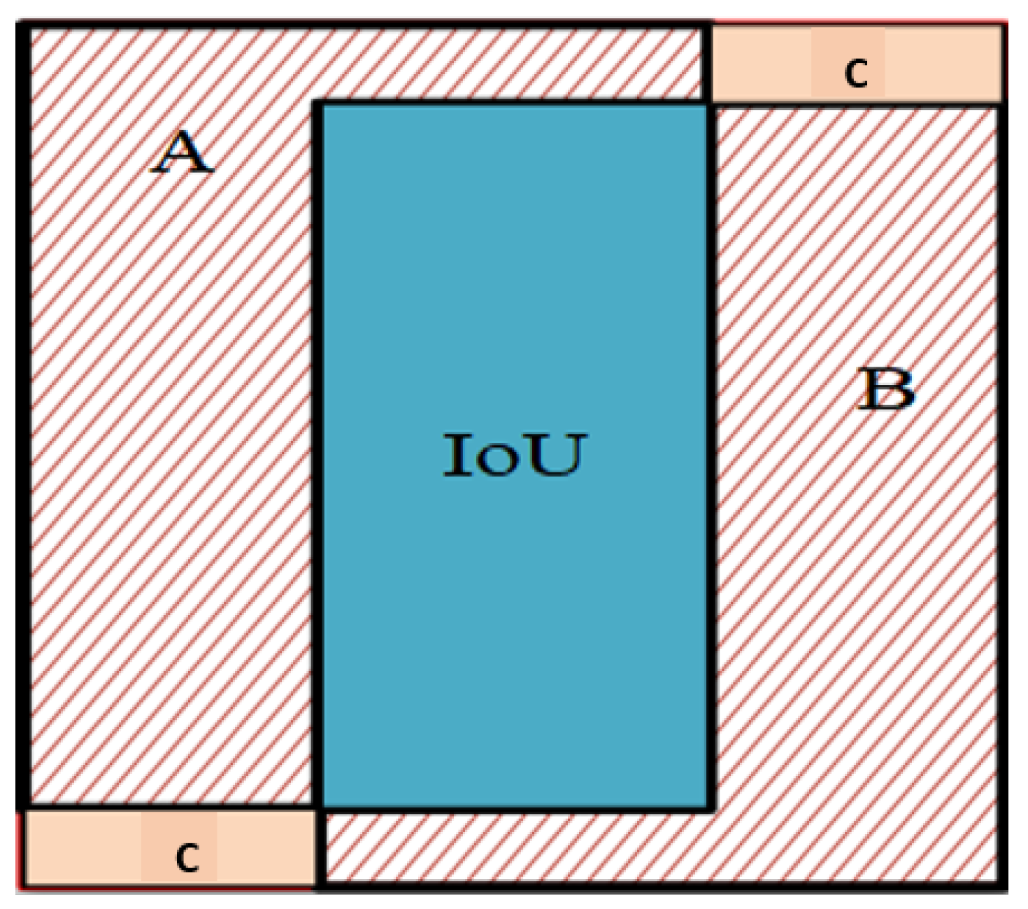
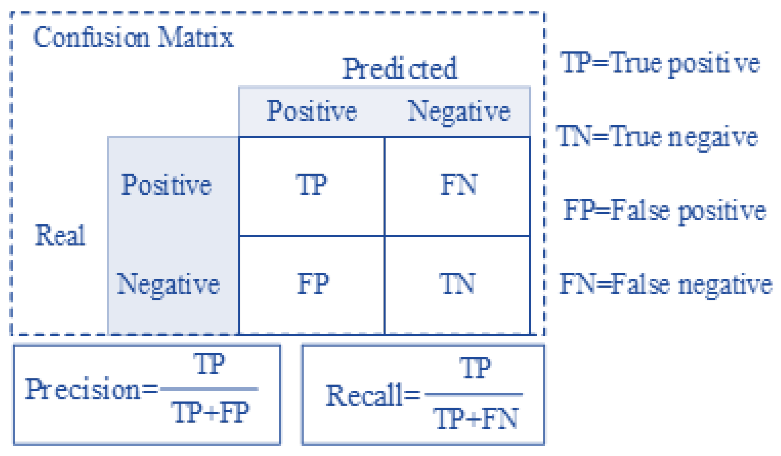
3.3. Classification and Regression Loss
3.4. Models
3.5. YOLOv5 and Variants
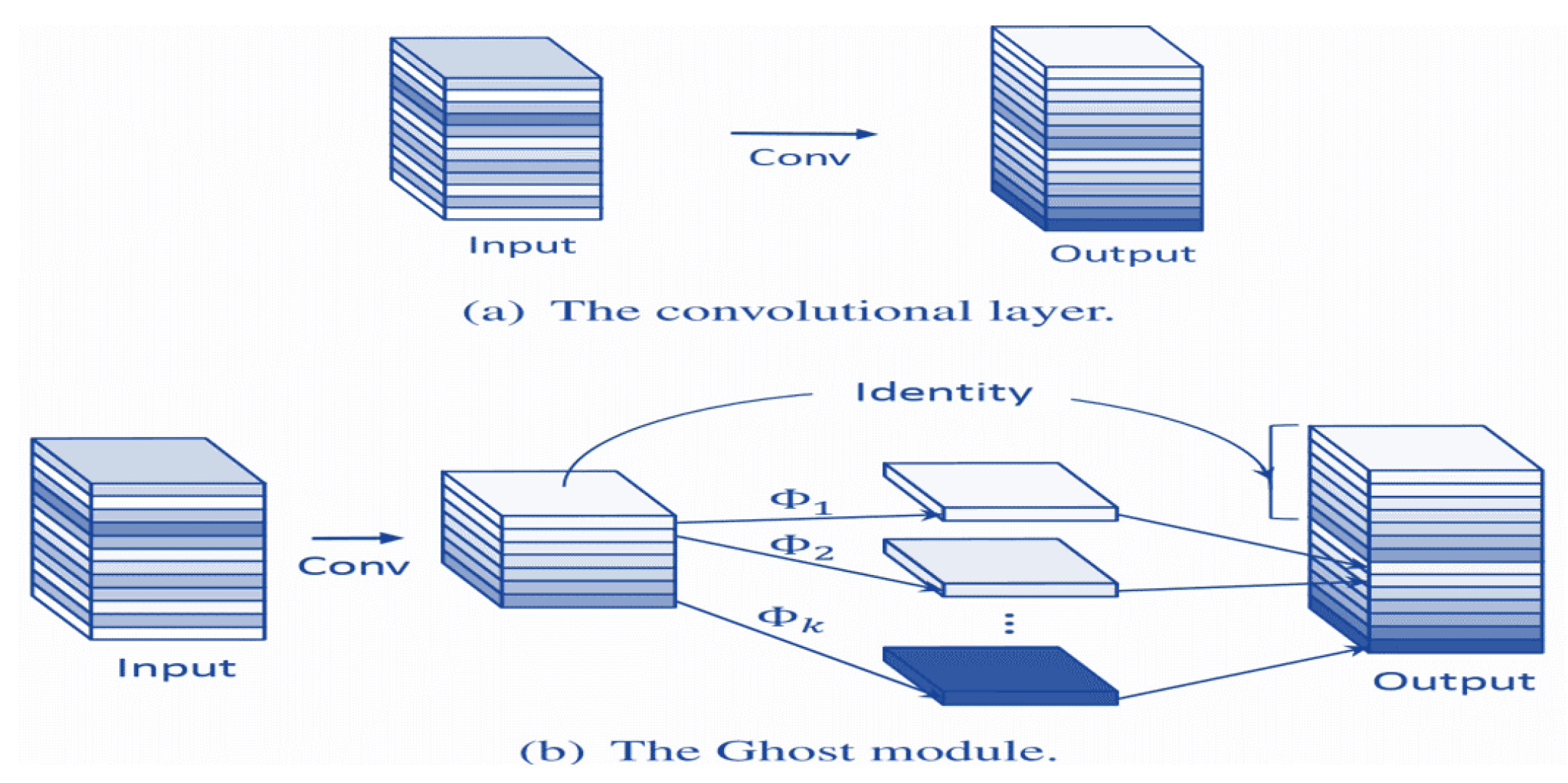
3.6. YOLOv5 Ghost
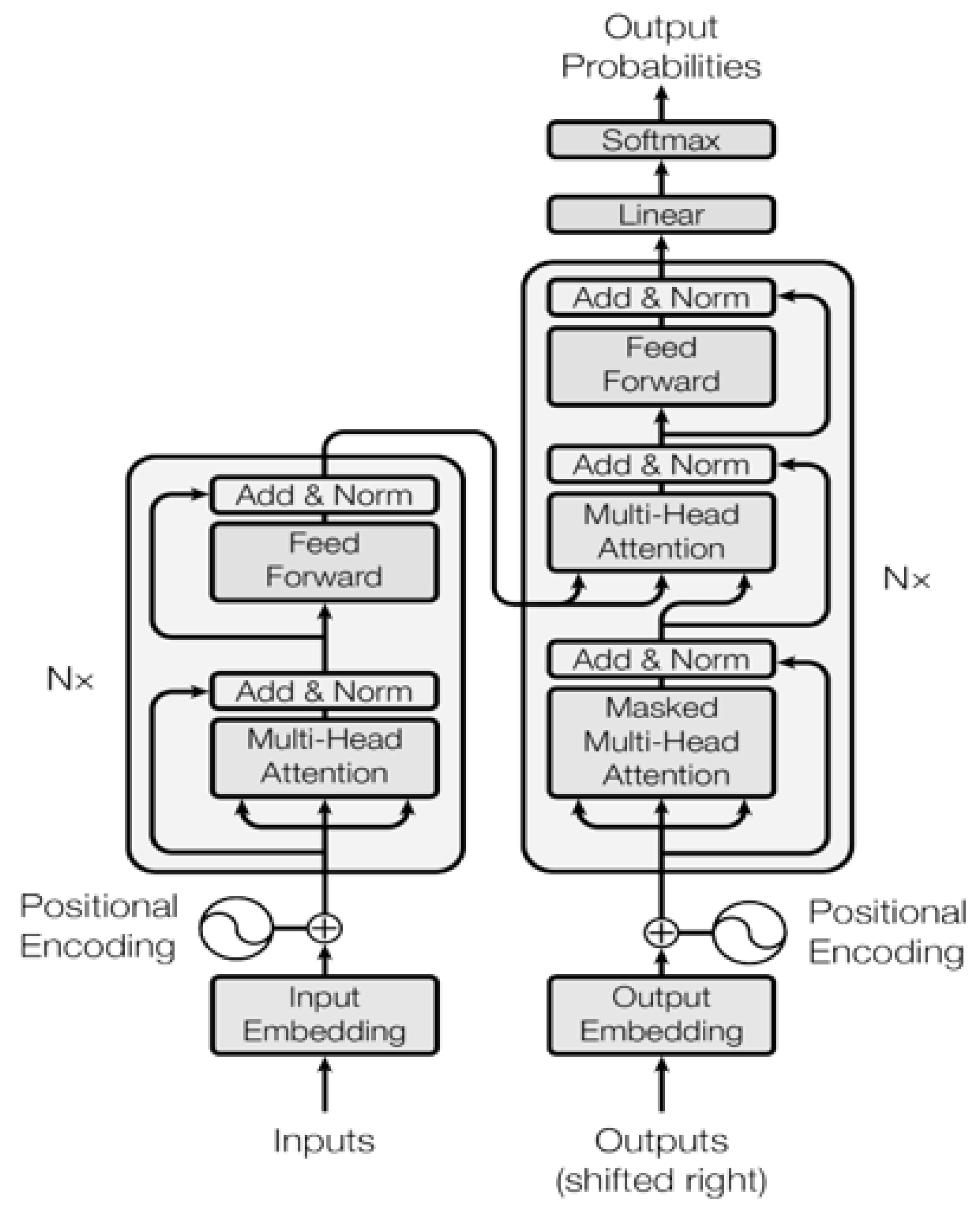
3.7. YOLOv5-Transformer
3.8. YOLOv5-Transformer-BiFPN
3.9. YOLOv5-FPN
4. Experimental and Discussion
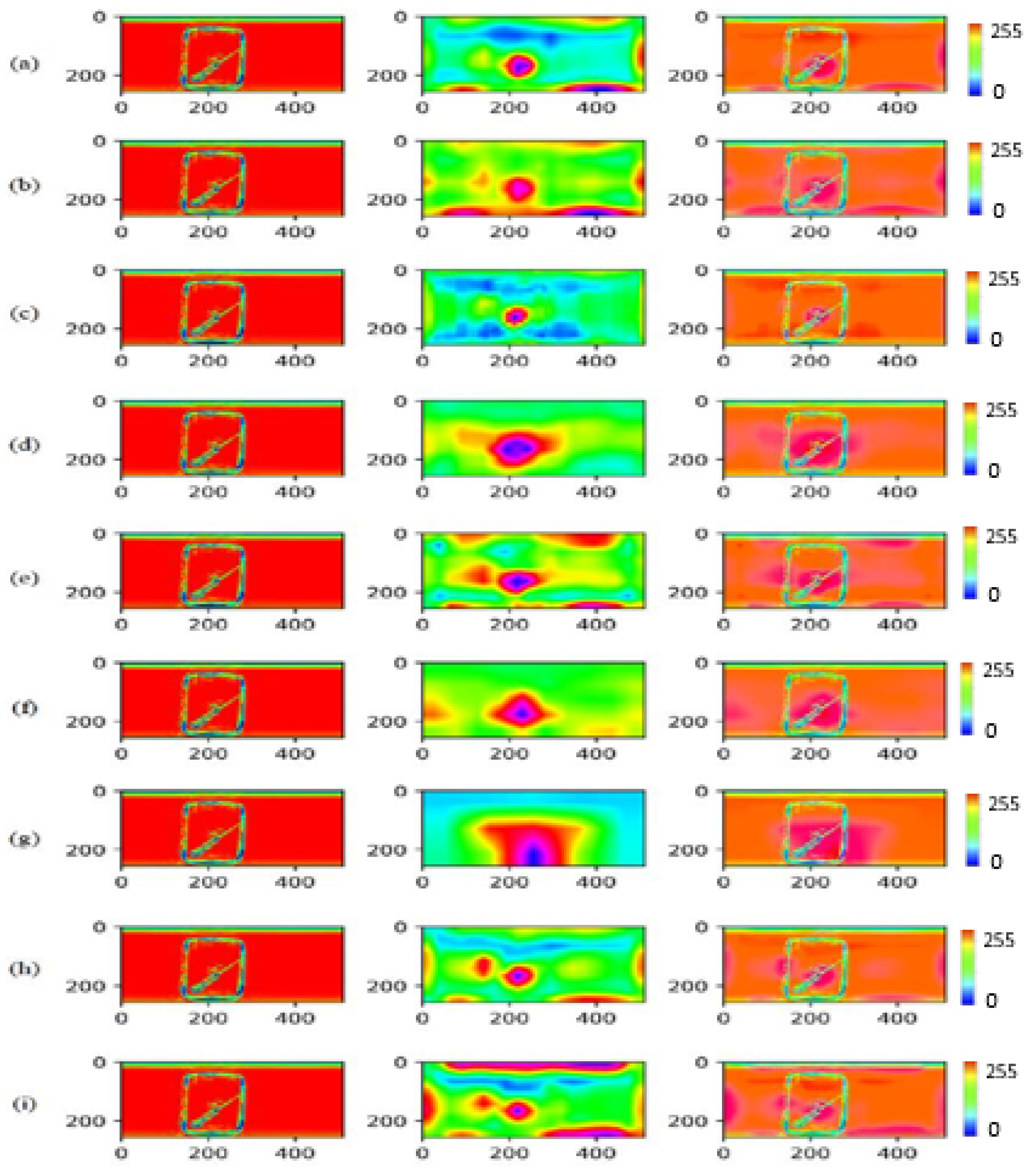
4.1. Terahertz Image Processing
4.2. Model Comparison
4.2.1. Experiment Results
4.2.2. Model Analysis
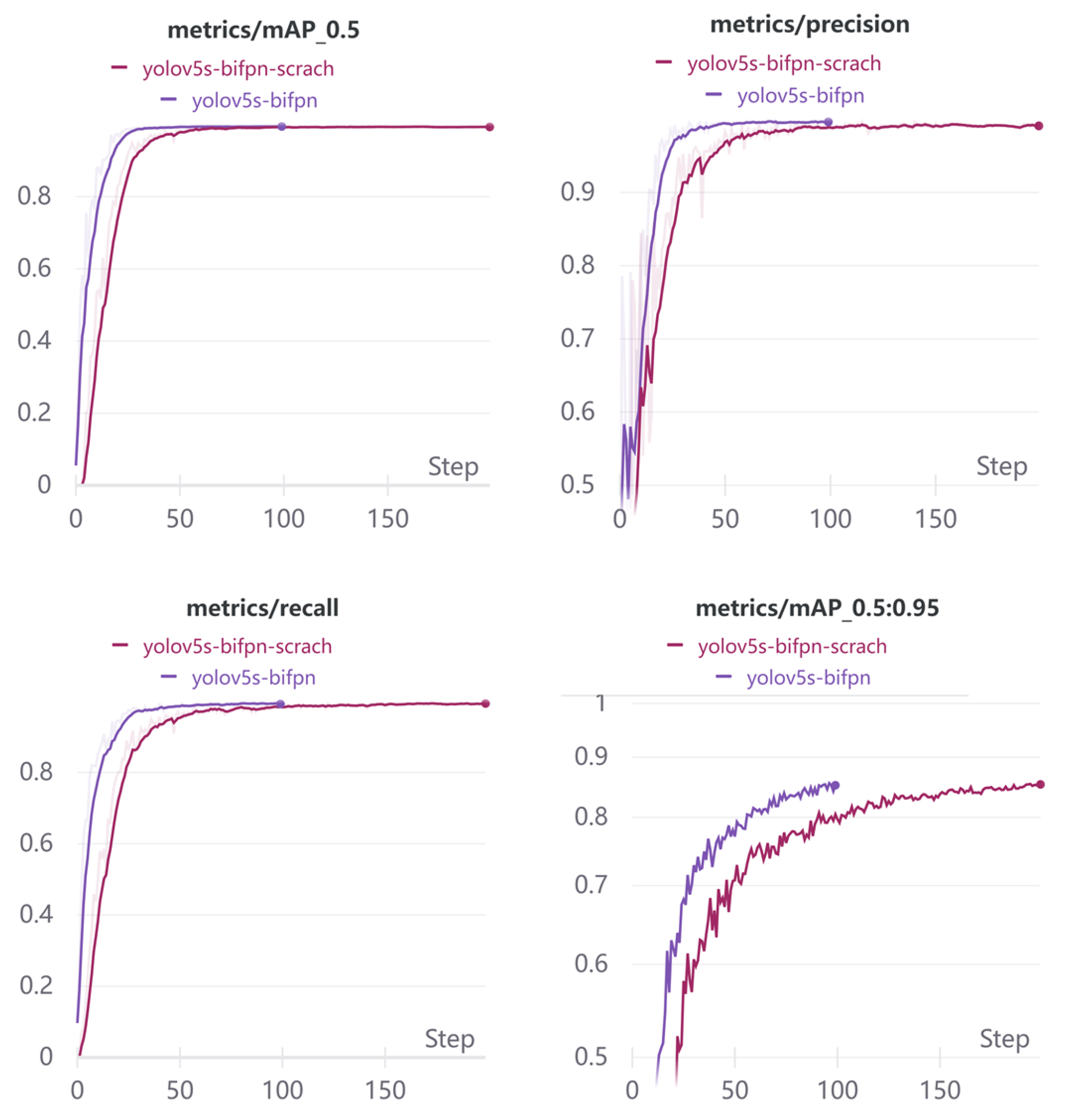
4.3. Model Transfer Learning
5. Conclusions
Author Contributions
Funding
Institutional Review Board Statement
Informed Consent Statement
Data Availability Statement
Conflicts of Interest
References
- Danso, S.; Liping, S.; Deng, H.; Odoom, J.; Appiah, E.; Etse, B.; Liu, Q. Denoising Terahertz Image Using Non-Linear Filters. Comput. Eng. Intell. Syst. 2021, 12. [Google Scholar] [CrossRef]
- Penkov, N.V.; Goltyaev, M.V.; Astashev, M.E.; Serov, D.A.; Moskovskiy, M.N.; Khort, D.O.; Gudkov, S.V. The Application of Terahertz Time-Domain Spectroscopy to Identification of Potato Late Blight and Fusariosis. Pathogens 2021, 10, 1336. [Google Scholar] [CrossRef] [PubMed]
- Hu, J.; Xu, Z.; Li, M.; He, Y.; Sun, X.; Liu, Y. Detection of Foreign-Body in Milk Powder Processing Based on Terahertz Imaging and Spectrum. J. Infrared Millimeter Terahertz Waves 2021, 42, 878–892. [Google Scholar] [CrossRef]
- Pan, S.; Qin, B.; Bi, L.; Zheng, J.; Yang, R.; Yang, X.; Li, Y.; Li, Z. An Unsupervised Learning Method for the Detection of Genetically Modified Crops Based on Terahertz Spectral Data Analysis. Secur. Commun. Netw. 2021, 2021, 5516253. [Google Scholar] [CrossRef]
- Ge, H.; Lv, M.; Lu, X.; Jiang, Y.; Wu, G.; Li, G.; Li, L.; Li, Z.; Zhang, Y. Applications of THz Spectral Imaging in the Detection of Agricultural Products. Photonics 2021, 8, 518. [Google Scholar] [CrossRef]
- Wang, L. Terahertz Imaging for Breast Cancer Detection. Sensors 2021, 21, 6465. [Google Scholar] [CrossRef]
- Yin, X.X.; Hadjiloucas, S.; Zhang, Y.; Tian, Z. MRI radiogenomics for intelligent diagnosis of breast tumors and accurate prediction of neoadjuvant chemotherapy responses—A review. Comput. Methods Programs Biomed. 2021, 214, 106510. [Google Scholar] [CrossRef]
- Kansal, P.; Gangadharappa, M.; Kumar, A. Terahertz E-Healthcare System and Intelligent Spectrum Sensing Based on Deep Learning. In Advances in Terahertz Technology and Its Applications; Springer: Berlin/Heidelberg, Germany, 2021; pp. 307–335. [Google Scholar]
- Liang, D.; Xue, F.; Li, L. Active Terahertz Imaging Dataset for Concealed Object Detection. arXiv 2021, arXiv:2105.03677. [Google Scholar]
- Owda, A.Y.; Salmon, N.; Owda, M. Indoor passive sensing for detecting hidden objects under clothing. In Proceedings of the Emerging Imaging and Sensing Technologies for Security and Defence VI, Online, 13–18 September 2021; Volume 11868, pp. 87–93. [Google Scholar]
- Dixit, N.; Mishra, A. Standoff Detection of Metallic Objects Using THz Waves. In ICOL-2019; Springer: Berlin/Heidelberg, Germany, 2021; pp. 911–914. [Google Scholar]
- Xu, F.; Huang, X.; Wu, Q.; Zhang, X.; Shang, Z.; Zhang, Y. YOLO-MSFG: Toward Real-Time Detection of Concealed Objects in Passive Terahertz Images. IEEE Sens. J. 2021, 22, 520–534. [Google Scholar] [CrossRef]
- Xie, X.; Lin, R.; Wang, J.; Qiu, H.; Xu, H. Target Detection of Terahertz Images Based on Improved Fuzzy C-Means Algorithm. In Proceedings of the 2021 Chinese Intelligent Systems Conference, Fuzhou, China, 16–17 October 2022; pp. 761–772. [Google Scholar]
- Wang, T.; Wang, K.; Zou, K.; Shen, S.; Yang, Y.; Zhang, M.; Yang, Z.; Liu, J. Virtual unrolling technology based on terahertz computed tomography. Opt. Lasers Eng. 2022, 151, 106924. [Google Scholar] [CrossRef]
- Mao, Q.; Liu, J.; Zhu, Y.; Lv, C.; Lu, Y.; Wei, D.; Yan, S.; Ding, S.; Ling, D. Developing industry-level terahertz imaging resolution using mathematical model. IEEE Trans. Terahertz Sci. Technol. 2021, 11, 583–590. [Google Scholar] [CrossRef]
- Widyastuti, R.; Yang, C.K. Cat’s nose recognition using you only look once (YOLO) and scale-invariant feature transform (SIFT). In Proceedings of the 2018 IEEE 7th Global Conference on Consumer Electronics (GCCE), Nara, Japan, 9–12 October 2018; pp. 55–56. [Google Scholar]
- Thu, M.; Suvonvorn, N. Pyramidal Part-Based Model for Partial Occlusion Handling in Pedestrian Classification. Adv. Multimed. 2020, 2020, 6153580. [Google Scholar] [CrossRef]
- Huang, B.; Chen, R.; Xu, W.; Zhou, Q.; Wang, X. Improved Fatigue Detection Using Eye State Recognition with HOG-LBP. In Proceedings of the 9th International Conference on Computer Engineering and Networks, Dubai, United Arab Emirates, 19–20 February 2022; pp. 365–374. [Google Scholar]
- Hazgui, M.; Ghazouani, H.; Barhoumi, W. Genetic programming-based fusion of HOG and LBP features for fully automated texture classification. Vis. Comput. 2021, 38, 457–476. [Google Scholar] [CrossRef]
- Pu, Y.; Apel, D.B.; Szmigiel, A.; Chen, J. Image recognition of coal and coal gangue using a convolutional neural network and transfer learning. Energies 2019, 12, 1735. [Google Scholar] [CrossRef] [Green Version]
- Zhou, Z.; Lu, Q.; Wang, Z.; Huang, H. Detection of Micro-Defects on Irregular Reflective Surfaces Based on Improved Faster R-CNN. Sensors 2019, 19, 5000. [Google Scholar] [CrossRef] [PubMed] [Green Version]
- Zhang, M.; Li, H.; Xia, G.; Zhao, W.; Ren, S.; Wang, C. Research on the application of deep learning target detection of engineering vehicles in the patrol and inspection for military optical cable lines by UAV. In Proceedings of the 2018 11th International Symposium on Computational Intelligence and Design (ISCID), Hangzhou, China, 8–9 December 2018; Volume 1, pp. 97–101. [Google Scholar]
- Li, W.; Feng, X.S.; Zha, K.; Li, S.; Zhu, H.S. Summary of Target Detection Algorithms. J. Phys. Conf. Ser. 2021, 1757, 012003. [Google Scholar] [CrossRef]
- Liang, F.; Zhou, Y.; Chen, X.; Liu, F.; Zhang, C.; Wu, X. Review of Target Detection Technology based on Deep Learning. In Proceedings of the 5th International Conference on Control Engineering and Artificial Intelligence, Online, 15 January 2021; pp. 132–135. [Google Scholar]
- Dai, Y.; Liu, Y.; Zhang, S. Mask R-CNN-based Cat Class Recognition and Segmentation. J. Phys. Conf. Ser. 2021, 1966, 012010. [Google Scholar] [CrossRef]
- Shi, J.; Zhou, Y.; Zhang, W.X.Q. Target detection based on improved mask rcnn in service robot. In Proceedings of the 2019 Chinese Control Conference (CCC), Guangzhou, China, 27–30 July 2019; pp. 8519–8524. [Google Scholar]
- Redmon, J.; Farhadi, A. YOLO9000: Better, faster, stronger. In Proceedings of the IEEE Conference on Computer Vision and Pattern Recognition, Honolulu, HI, USA, 21–26 July 2017; pp. 7263–7271. [Google Scholar]
- Loey, M.; Manogaran, G.; Taha, M.H.N.; Khalifa, N.E.M. Fighting against COVID-19: A novel deep learning model based on YOLO-v2 with ResNet-50 for medical face mask detection. Sustain. Cities Soc. 2021, 65, 102600. [Google Scholar] [CrossRef]
- Kumar, A.; Kumar, A.; Bashir, A.K.; Rashid, M.; Kumar, V.A.; Kharel, R. Distance based pattern driven mining for outlier detection in high dimensional big dataset. ACM Trans. Manag. Inf. Syst. 2021, 13, 1–17. [Google Scholar] [CrossRef]
- Chien, S.; Chen, Y.; Yi, Q.; Ding, Z. Development of Automated Incident Detection System Using Existing ATMS CCTV; Purdue University: West Lafayette, IN, USA, 2019. [Google Scholar]
- Jaszewski, M.; Parameswaran, S.; Hallenborg, E.; Bagnall, B. Evaluation of maritime object detection methods for full motion video applications using the pascal voc challenge framework. In Proceedings of the Video Surveillance and Transportation Imaging Applications, San Francisco, CA, USA, 8–12 February 2015; Volume 9407, p. 94070Y. [Google Scholar]
- Zhou, P.; Ni, B.; Geng, C.; Hu, J.; Xu, Y. Scale-transferrable object detection. In Proceedings of the IEEE Conference on Computer Vision and Pattern Recognition, Salt Lake City, UT, USA, 18–22 June 2018; pp. 528–537. [Google Scholar]
- Lin, T.Y.; Maire, M.; Belongie, S.; Hays, J.; Perona, P.; Ramanan, D.; Dollár, P.; Zitnick, C.L. Microsoft coco: Common objects in context. In Proceedings of the European Conference on Computer Vision, Zurich, Switzerland, 6–12 September 2014; pp. 740–755. [Google Scholar]
- Ping-Yang, C.; Hsieh, J.W.; Gochoo, M.; Chen, Y.S. Light-Weight Mixed Stage Partial Network for Surveillance Object Detection with Background Data Augmentation. In Proceedings of the 2021 IEEE International Conference on Image Processing (ICIP), Anchorage, AK, USA, 19–22 September 2021; pp. 3333–3337. [Google Scholar]
- Liao, J.; Zou, J.; Shen, A.; Liu, J.; Du, X. Cigarette end detection based on EfficientDet. J. Phys. Conf. Ser. 2021, 1748, 062015. [Google Scholar] [CrossRef]
- Wang, K.; Liew, J.H.; Zou, Y.; Zhou, D.; Feng, J. Panet: Few-shot image semantic segmentation with prototype alignment. In Proceedings of the IEEE/CVF International Conference on Computer Vision, Seoul, Korea, 27 October–2 November 2019; pp. 9197–9206. [Google Scholar]
- Chen, Z.; Cong, R.; Xu, Q.; Huang, Q. DPANet: Depth potentiality-aware gated attention network for RGB-D salient object detection. IEEE Trans. Image Process. 2020, 30, 7012–7024. [Google Scholar] [CrossRef] [PubMed]
- Wang, C.Y.; Liao, H.Y.M.; Wu, Y.H.; Chen, P.Y.; Hsieh, J.W.; Yeh, I.H. CSPNet: A new backbone that can enhance learning capability of CNN. In Proceedings of the IEEE/CVF Conference on Computer Vision and Pattern Recognition Workshops, Seattle, WA, USA, 14–19 June 2020; pp. 390–391. [Google Scholar]
- Rezatofighi, H.; Tsoi, N.; Gwak, J.; Sadeghian, A.; Reid, I.; Savarese, S. Generalized intersection over union: A metric and a loss for bounding box regression. In Proceedings of the IEEE/CVF International Conference on Computer Vision, Seoul, Korea, 27 October–2 November 2019; pp. 658–666. [Google Scholar]
- Xu, R.; Lin, H.; Lu, K.; Cao, L.; Liu, Y. A forest fire detection system based on ensemble learning. Forests 2021, 12, 217. [Google Scholar] [CrossRef]
- Han, K.; Wang, Y.; Tian, Q.; Guo, J.; Xu, C.; Xu, C. Ghostnet: More features from cheap operations. In Proceedings of the IEEE/CVF Conference on Computer Vision and Pattern Recognition Workshops, Seattle, WA, USA, 14–19 June 2020; pp. 1580–1589. [Google Scholar]
- Zhu, X.; Lyu, S.; Wang, X.; Zhao, Q. TPH-YOLOv5: Improved YOLOv5 based on transformer prediction head for object detection on drone-captured scenarios. In Proceedings of the Proceedings of the IEEE/CVF International Conference on Computer Vision; Montreal, BC, Canada, 11–17 October 2021, pp. 2778–2788.
- Zolotareva, E.; Tashu, T.M.; Horváth, T. Abstractive Text Summarization using Transfer Learning. In Proceedings of the ITAT, Oravská Lesná, Slovakia, 18–22 September 2020; pp. 75–80. [Google Scholar]
- Guo, Z.; Wang, C.; Yang, G.; Huang, Z.; Li, G. MSFT-YOLO: Improved YOLOv5 Based on Transformer for Detecting Defects of Steel Surface. Sensors 2022, 22, 3467. [Google Scholar] [CrossRef] [PubMed]
- Qiu, Z.; Zhao, Z.; Chen, S.; Zeng, J.; Huang, Y.; Xiang, B. Application of an Improved YOLOv5 Algorithm in Real-Time Detection of Foreign Objects by Ground Penetrating Radar. Remote Sens. 2022, 14, 1895. [Google Scholar] [CrossRef]
- Danso, S.A.; Liping, S.; Deng, H.; Odoom, J.; Chen, L.; Xiong, Z.G. Optimizing Yolov3 detection model using terahertz active security scanned low-resolution images. Theor. Appl. Sci. 2021, 3, 235–253. [Google Scholar] [CrossRef]


| Class | Screwdriver | Blade | Knife | Scissors | Boardmarker | Mobile Phone | Wireless Mouse | Water Bottle |
|---|---|---|---|---|---|---|---|---|
| No. | 65 | 21 | 66 | 59 | 40 | 40 | 40 | 40 |
| Avg. bounding box | 108 px × 84 px | 36 px × 35 px | 89 px × 75 px | 104 px × 91 px | 78 px × 68 px | 110 px × 87 px | 70 px × 75 px | 118 px × 91 px |
| Model | Precision | Recall | mAP@0.5 | mAP@0.5:0.95 |
|---|---|---|---|---|
| YOLOv5-BiFPN (ours) | 0.991 | 0.991 | 0.993 | 0.857 |
| YOLOv5 | 0.99 | 0.996 | 0.995 | 0.862 |
| YOLOv5-fpn | 0.994 | 0.996 | 0.995 | 0.845 |
| YOLOv5-ghost | 0.987 | 0.983 | 0.992 | 0.855 |
| YOLOv5-p2 | 0.98 | 0.974 | 0.981 | 0.835 |
| YOLOv5-p7 | 0.99 | 0.988 | 0.993 | 0.847 |
| YOLOv5-p6 | 0.991 | 0.98 | 0.99 | 0.85 |
| YOLOv5-Transformer | 0.989 | 0.994 | 0.994 | 0.853 |
| YOLOv5-Transformer-BiFPN | 0.993 | 0.987 | 0.994 | 0.854 |
| CSPDarknet53-PANet-SPP [46] | 0.804 |
| Model | Precision | Recall | mAP@0.5 | mAP@0.5:0.95 |
|---|---|---|---|---|
| all | 0.991 | 0.991 | 0.993 | 0.857 |
| screw_drive | 0.975 | 0.987 | 0.992 | 0.705 |
| blade | 0.992 | 1 | 0.995 | 0.793 |
| knife | 0.989 | 0.988 | 0.995 | 0.782 |
| scissors | 0.986 | 0.99 | 0.995 | 0.832 |
| board_marker | 0.995 | 1 | 0.995 | 0.914 |
| mobile_phone | 0.995 | 1 | 0.995 | 0.966 |
| wireless_mouse | 0.994 | 1 | 0.995 | 0.941 |
| water_bottle | 0.995 | 1 | 0.995 | 0.963 |
| Model | Precision | Recall | mAP@0.5 | mAP@0.5:0.95 |
|---|---|---|---|---|
| all | 0.992 | 0.998 | 0.995 | 0.874 |
| screw_drive | 0.987 | 0.987 | 0.994 | 0.739 |
| blade | 0.985 | 1 | 0.995 | 0.792 |
| knife | 0.982 | 1 | 0.994 | 0.786 |
| scissors | 1 | 1 | 0.995 | 0.861 |
| board_marker | 0.996 | 1 | 0.995 | 0.933 |
| mobile_phone | 0.995 | 1 | 0.995 | 0.967 |
| wireless_mouse | 0.994 | 1 | 0.995 | 0.931 |
| water_bottle | 0.996 | 1 | 0.995 | 0.982 |
Publisher’s Note: MDPI stays neutral with regard to jurisdictional claims in published maps and institutional affiliations. |
© 2022 by the authors. Licensee MDPI, Basel, Switzerland. This article is an open access article distributed under the terms and conditions of the Creative Commons Attribution (CC BY) license (https://creativecommons.org/licenses/by/4.0/).
Share and Cite
Danso, S.A.; Shang, L.; Hu, D.; Odoom, J.; Liu, Q.; Nana Esi Nyarko, B. Hidden Dangerous Object Recognition in Terahertz Images Using Deep Learning Methods. Appl. Sci. 2022, 12, 7354. https://doi.org/10.3390/app12157354
Danso SA, Shang L, Hu D, Odoom J, Liu Q, Nana Esi Nyarko B. Hidden Dangerous Object Recognition in Terahertz Images Using Deep Learning Methods. Applied Sciences. 2022; 12(15):7354. https://doi.org/10.3390/app12157354
Chicago/Turabian StyleDanso, Samuel Akwasi, Liping Shang, Deng Hu, Justice Odoom, Quancheng Liu, and Benedicta Nana Esi Nyarko. 2022. "Hidden Dangerous Object Recognition in Terahertz Images Using Deep Learning Methods" Applied Sciences 12, no. 15: 7354. https://doi.org/10.3390/app12157354
APA StyleDanso, S. A., Shang, L., Hu, D., Odoom, J., Liu, Q., & Nana Esi Nyarko, B. (2022). Hidden Dangerous Object Recognition in Terahertz Images Using Deep Learning Methods. Applied Sciences, 12(15), 7354. https://doi.org/10.3390/app12157354