Empirical Perturbation Analysis of Two Adversarial Attacks: Black Box versus White Box

Abstract

Through the addition of humanly imperceptible noise to an image classified as belonging to a category $c_a$, targeted adversarial attacks can lead convolutional neural networks (CNNs) to classify a modified image as belonging to any predefined target class $c_t\ne c_a$. To achieve a better understanding of the inner workings of adversarial attacks, this study analyzes the adversarial images created by two completely opposite attacks against 10 ImageNet-trained CNNs. A total of $2\times 437$ adversarial images are created by ${\mathrm{EA}}^{\mathrm{target},\mathcal{C}}$, a black-box evolutionary algorithm (EA), and by the basic iterative method (BIM), a white-box, gradient-based attack. We inspect and compare these two sets of adversarial images from different perspectives: the behavior of CNNs at smaller image regions, the image noise frequency, the adversarial image transferability, the image texture change, and penultimate CNN layer activations. We find that texture change is a side effect rather than a means for the attacks and that $c_t$-relevant features only build up significantly from image regions of size $56\times 56$ onwards. In the penultimate CNN layers, both attacks increase the activation of units that are positively related to $c_t$ and units that are negatively related to $c_a$. In contrast to ${\mathrm{EA}}^{\mathrm{target},\mathcal{C}}$’s white noise nature, BIM predominantly introduces low-frequency noise. BIM affects the original $c_a$ features more than ${\mathrm{EA}}^{\mathrm{target},\mathcal{C}}$, thus producing slightly more transferable adversarial images. However, the transferability with both attacks is low, since the attacks’ $c_t$-related information is specific to the output layers of the targeted CNN. We find that the adversarial images are actually more transferable at regions with sizes of $56\times 56$ than at full scale.

1. Introduction

Trained convolutional neural networks (CNNs) are among the dominant and most accurate tools for automatic image classification [1]. Nevertheless, they can be fooled by attacks [2] following particular scenarios, which can lead to classification errors in adversarial images. In the present work, we mainly consider the target scenario. Given a trained CNN $\mathcal{C}$ and an ancestor image $\mathcal{A}$ classified by $\mathcal{C}$ as belonging to category $c_a$, it first consists of choosing a target category $c_t\ne c_a$. Then, the attack perturbs $\mathcal{A}$ to create an adversarial image $\mathcal{D}\left(\mathcal{A}\right)$, which not only is classified by $\mathcal{C}$ as belonging to category $c_t$ but also is humanly indistinguishable from $\mathcal{A}$.

Attacks are classified into three groups depending on the amount of information that the attackers have at their disposal. Gradient-based attacks (see e.g., [3,4,5,6,7]) have complete knowledge of $\mathcal{C}$, its explicit architecture, its layers, and their respective weights. The insider knowledge of the CNN is much more limited for transfer-based attacks (see e.g., [8,9,10]). They create a model mirroring $\mathcal{C}$, which they attack with gradient-based methods, leading to adversarial images that also fool $\mathcal{C}$. Score-based attacks (see [11,12]) are the least demanding of all. The training data, model architecture, and parameters of the CNN are unknown to them. They only require $\mathcal{C}$’s predicted output label values for either all or a subset of object categories.

This study aims to gain insights into the functioning of adversarial attacks by analyzing the adversarial images, on the one hand, and the reactions of CNNs when exposed to adversarial images, on the other hand. These analyses and comparisons are performed from different perspectives: the behavior while looking at smaller regions, the noise frequency, the transferability, the changes in image texture, and the penultimate layer activations. The reasons for considering these perspectives are as follows. The first question we attempt to answer is whether adversarial attacks make use of texture change to fool CNNs. This texture issue is related to the frequency of the noise in the sense that changes in the image texture are reflected by the input of high-frequency noise [13]. This issue is also related to what occurs at smaller image regions, as texture modifications should also be noticed at these levels. The transferability issue measures the extent to which the adversarial noise is specific to the attacked CNN or to the training data. Finally, studying the behavior of the penultimate layers of the addressed CNNs provides a close look at the direction of the adversarial noise with respect to each object category.

This insight is addressed through a thorough experimental study. We selected 10 CNNs that are very diverse in terms of architecture, number of layers, etc. These CNNs are trained on the ImageNet dataset to sort images with sizes of $224\times 224$ into 1000 categories. We then intentionally chose two attacks that are on opposing edges of the attacks’ classification. More precisely, here, we consider the gradient-based BIM [3] and the score-based ${\mathrm{EA}}^{\mathrm{target},\mathcal{C}}$ [14,15,16,17], with both having high success rates against CNNs trained on ImageNet [14,18].

We run these two algorithms to fool the 10 CNNs, with the additional very-demanding requirement that, for an image to be considered adversarial, its $c_t$-label value should exceed $0.999$. We start with 10 random pairs of ancestor and target categories $(c_a,c_t)$ and 10 random ancestor images in each $c_a$, hence 100 ancestor images altogether. Out of the 1000 performed runs per attack, the two attacks succeeded for 84 common ancestors, leading to 2 distinct groups (one for each attack) of 437 adversarial images coming from these 84 convenient ancestors. The $2\times 437$ adversarial images and the 10 CNNs are then analyzed and compared from the abovementioned perspectives. Each of these perspectives is addressed in a dedicated section containing the specific obtained outcomes.

We first analyze whether the adversarial noise introduced by the EA and BIM has an adversarial impact at regions of smaller sizes. We also explore whether this local noise alone is sufficient to mislead the CNN, either individually or globally, but in a shuffled manner. To the best of our knowledge, we are the first to study the image level at which the attacks’ noise becomes adversarial.

Additionally, we provide a visualization of the noise that the EA and BIM add to an ancestor image to produce an adversarial image. In particular, we identify the frequencies of the noise introduced by the EA and BIM and, among them, those that are key to the adversarial nature of the images created by each of the two attacks. In contrast, in [19], the authors studied the noise introduced by several attacks and found that it is in the high-frequency range; their study was limited to attacks on CNNs trained on Cifar-10. Since Cifar-10 contains images of considerably smaller sizes than the images of ImageNet, the results of that noise frequency study differed considerably. Another study [20], performed on both abovementioned datasets, found that adversarial attacks are not necessarily a high-frequency phenomenon. Here, we further prove that the EA attack introduces white noise, while the BIM attack actually introduces predominantly low-frequency noise. Moreover, with both attacks, we find that, irrespective of the types of noise they introduce, the lower part of the spectrum is responsible for carrying adversarial information.

We next explore the texture changes introduced by the attacks in relation to the transferability of the adversarial images from one CNN to another. The issue is to clarify whether adversarial images are specific to their targeted CNN or whether they contain rather general features that are perceivable by others. It has been proven that ImageNet-trained CNNs are biased towards texture [21], while CNNs that have been adversarially trained to become robust against attacks have a bias towards shape [22]. However, here, we attempt to find whether texture change is an underlying mechanism of attacks, to evaluate the degree to which it participates in fooling a CNN, and to check whether CNNs with differing amounts of texture bias agree on which image modifications have the largest adversarial impact. We find that texture change takes place in the attacks’ perturbation of the images, but that this texture change is not necessarily responsible for fooling the CNNs. However, our results show that adversarial images are more likely to transfer to CNNs that have higher texture biases.

Previous work on the transferability of a gradient-based FGSM [4] attack has proven that, while untargeted attacks transfer easily, targeted attacks have a very low transferability rate [9]. Here, we provide the first study of the transferability of a targeted gradient-based BIM as well as of a targeted black-box EA. We find that, in both cases, transferability is extremely low.

In another direction related to transferability, the authors of [23] specifically perturbed certain features of intermediate CNN layers and compared the transferability of the adversarial images targeting different intermediate features. They proved that perturbing features in early CNN layers result in more transferability than perturbing features in later CNN layers. It is also known that early CNN layers capture more textural information found in smaller image regions, whereas later CNN layers capture more shape-related information found in larger image regions [24]. Considering the two statements above, we create the EA and BIM adversarial images that target the last CNN layers and explore whether the adversarial noise at smaller image regions is less CNN-specific, hence more transferable, than the noise at the full-image scale. This issue is addressed in two ways. First, we check whether and how a modification of the adversarial noise intensity affects the $c_a$ and the $c_t$-label values predicted by a CNN when fed with a different CNN’s adversarial image, and the influence of shuffling in this process. Second, we keep the adversarial noise as it is (meaning without changing its intensity), and we check whether adversarial images are more likely to transfer when they are shuffled.

Finally, we delve inside the CNNs and study the changes that adversarial images produce in the activation of the CNNs’ penultimate layers. A somewhat similar study was performed in [25], where the activations at all layers were visualized for one CNN trained on Cifar-10. Here, rather than performing a visualization of the intermediate activations, we attempt to quantify the precise nature of the changes made on the path to reaching a high probability for the target class in the final layer. We find that both attacks introduce noise that increases the activation of the positively related $c_t$ units and (perhaps simultaneously) increases the activation of negatively related $c_a$ units.

The paper is organized as follows: Section 2 defines the concept of a $\tau$-strong adversarial image and briefly describes the two attacks used here, namely the EA and BIM. We explain the criteria leading to the selection of the 10 CNNs, the ancestor and target categories, as well as the choice of the ancestor images in each category. In Section 3, we study the impact of the two attacks’ adversarial noise at smaller image regions. In Section 4, we perform the study of the noise frequency. Section 5 explores the texture changes introduced by the two attacks, while the transferability of their generated adversarial images is pursued in Section 6. Moreover, the activation of the CNNs’ penultimate layers is analyzed in Section 7. The concluding Section 8 summarizes our results and describes some future research directions. This study is completed by two appendices. 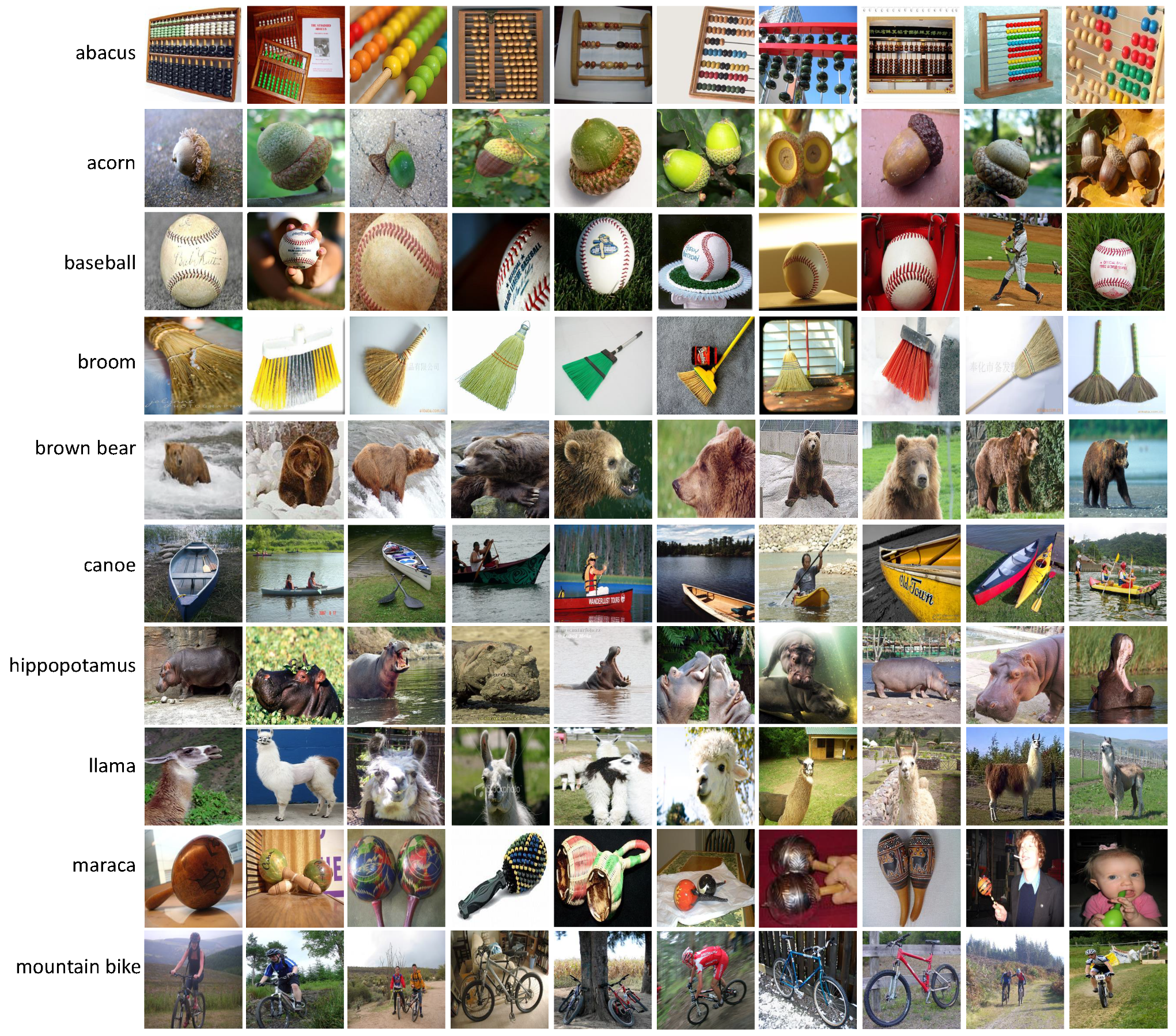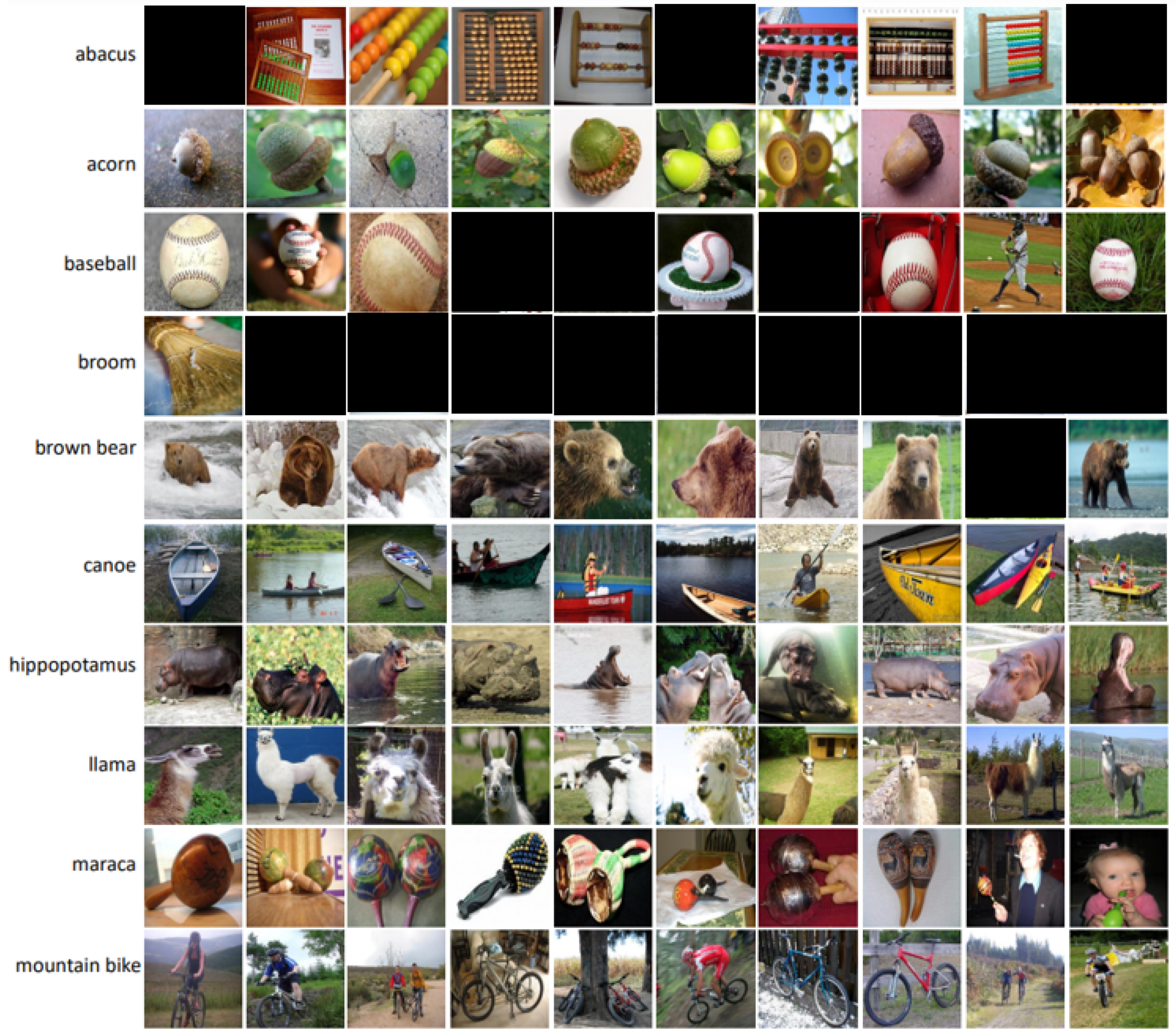Appendix A displays all considered ancestors, the convenient ancestors, and some $0.999$-strong adversarial images obtained by the EA and BIM. Appendix B contains a series of tables and graphs supporting our findings.

2. Adversarial Images Created by BIM and ${\mathrm{EA}}^{\mathrm{target},\mathcal{C}}$

This section first specifies the requirements for a successful targeted attack (Section 2.1). We then list both the 10 CNNs and the (ancestor and target) category pairs on which the targeted attacks are performed (Section 2.2). Since this paper’s focus is on performing experiments with the adversarial images rather than on evaluating the functioning or performance of the attacks, we only provide a brief overview of the two algorithms used here, namely ${\mathrm{EA}}^{\mathrm{target},\mathcal{C}}$ and BIM (Section 2.3). Lastly, we specify the parameters used by ${\mathrm{EA}}^{\mathrm{target},\mathcal{C}}$ and BIM to construct the adversarial images used in the remainder of this study (Section 2.4).

2.1. Targeted Attack: $\tau$-Strong Adversarial Images

Let $\mathcal{C}$ be a CNN trained on the ImageNet [26] dataset to label images into 1000 categories $c_1,\cdots ,c_{1000}$. Let $\mathcal{A}$ be an ancestor image that both a human and $\mathcal{C}$ label as belonging to the same category $c_a$. Performing a targeted attack on this CNN involves choosing a target category $c_t\ne c_a$ and perturbing $\mathcal{A}$ to create an image ${\mathcal{D}}_{a,t}\left(\mathcal{A}\right)$, which is adversarial for $\mathcal{C}$ in the following sense. First, one requires that $\mathcal{C}$ classifies ${\mathcal{D}}_{a,t}\left(\mathcal{A}\right)$ as belonging to $c_t$. Thus, the following equation holds:

$$t=\arg {\max }_{1\le j\le 1000}\left({\mathit{o}}_{{\mathcal{D}}_{a,t}\left(\mathcal{A}\right)}^{\mathcal{C}}\left[j\right]\right),$$

(1)

where ${\mathit{o}}_{{\mathcal{D}}_{a,t}\left(\mathcal{A}\right)}^{\mathcal{C}}$ is the classification output vector produced by $\mathcal{C}$ when fed with ${\mathcal{D}}_{a,t}\left(\mathcal{A}\right)$. Although this condition alone may be considered sufficient, we set an additional requirement that the $c_t$-label value of the output vector satisfies the inequality ${\mathit{o}}_{{\mathcal{D}}_{a,t}\left(\mathcal{A}\right)}^{\mathcal{C}}\left[t\right]\ge \tau$ for $\tau$ at a fixed constant threshold value $\in [0,1]$ that is sufficiently close to 1 to guarantee confident adversarial classification. Second, we require the image ${\mathcal{D}}_{a,t}\left(\mathcal{A}\right)$ to remain close to the ancestor image $\mathcal{A}$ so that a human would not be able to distinguish between ${\mathcal{D}}_{a,t}\left(\mathcal{A}\right)$ and $\mathcal{A}$. An image ${\mathcal{D}}_{a,t}\left(\mathcal{A}\right)$ satisfying these conditions is a $\tau$-strong adversarial image for the $(c_a,c_t)$ target scenario performed on $\mathcal{C}$ with the original image $\mathcal{A}$.

2.2. Selected CNNs, and Ancestor and Target Categories

We challenge a significant series of well-known CNNs that cover a large part of the existing deep learning approaches to object recognition. For practical reasons and for comparison purposes, we require the pre-trained versions to be available in the PyTorch [27] library and that they handle images of similar sizes. These criteria led us to select the following 10 CNNs, trained on ImageNet, that handle images of size $224\times 224$: ${\mathcal{C}}_1=$ DenseNet-121 [28], ${\mathcal{C}}_2=$ DenseNet-169 [28], ${\mathcal{C}}_3=$ DenseNet-201 [28], ${\mathcal{C}}_4=$ MobileNet [29], ${\mathcal{C}}_5=$ MNASNet [30], ${\mathcal{C}}_6=$ ResNet-50 [31], ${\mathcal{C}}_7=$ ResNet-101 [31], ${\mathcal{C}}_8=$ ResNet-152 [31], ${\mathcal{C}}_9=$ VGG-16 [32], ${\mathcal{C}}_{10}=$ VGG-19 [32] (two additional CNNs, BagNet-17 [33] and ResNet-50-SIN [21], are considered in Section 5 for the reasons explained thereof).

Among the 1000 categories of ImageNet, we randomly pick ten ancestor $a_1,\cdots ,a_{10}$ and ten target categories $t_1,\cdots ,t_{10}$. The results are listed in

Table 1. For $1\le q\le 10$, the second row gives the ancestor category $c_{a_q}$ and its index number $a_q$ among the categories of ImageNet (Mutatis mutandis for the target categories, third row).

q	1	2	3	4	5	6	7	8	9	10
$c_{a_q}$ $a_q$	abacus 398	acorn 988	baseball 429	broom 462	brown bear 294	canoe 472	hippopotamus 344	llama 355	maraca 641	mountain bike 671
$c_{t_q}$ $t_q$	bannister 421	rhinoceros beetle 306	ladle 618	dingo 273	pirate 724	Saluki 176	trifle 927	agama 42	conch 112	strainer 828

. For each (ancestor and target) pair $(c_{a_q},c_{t_q})$ (with $1\le q\le 10$), we randomly select 10 ancestor images ${\mathcal{A}}_q^p$ (with $1\le p\le 10$), resized to $224\times 224$ using bilinear interpolation if necessary. These 100 ancestor images, shown in Figure A1 in Appendix A, are labeled by the 10 CNNs as $a_q$ in 97% cases, with negligible $c_{t_q}$-label values (approximately between 9 × 10⁻¹¹ and 2 × 10⁻³). Two different algorithms are used to perform targeted attacks on all 10 CNNs, all 10 $(c_{a_q},c_{t_q})$ ($1\le q\le 10$) pairs, and all 10 ${\mathcal{A}}_q^p$ ($1\le p\le 10$).

2.3. Design of ${\mathit{EA}}^{\mathit{target},\mathcal{C}}$ and of BIM

Given a trained CNN $\mathcal{C}$, this section summarizes the key features of the ${\mathrm{EA}}^{\mathrm{target},\mathcal{C}}$ [14] (see also [15,16,17]) and BIM [3]. In both cases, their purpose is to evolve an ancestor image $\mathcal{A}$ into a $\tau$-strong adversarial image (for some convenient value of $\tau$) that deceives $\mathcal{C}$ at image classification. However, their methods differ, as summarized below.

2.3.1. ${\mathrm{EA}}^{\mathrm{target},\mathcal{C}}$

The pseudo-code for this evolutionary algorithm is given in Algorithm A1 (see Appendix A.1). The EA requires no knowledge of the CNN’s architecture or parameters, since it only makes use of a network’s input and output. At the beginning of the algorithm, identical copies of the original image are used to create the initial EA population. Throughout generations, the only information extracted from the CNNs are the $c_t$ probabilities of the individuals. The objective of evolving an individual $ind$ towards an image classified as belonging to $c_t$ is encoded in the fitness function $fit\left(ind\right)={\mathit{o}}_{ind}^{\mathcal{C}}\left[t\right]$. Throughout the evolution, the individuals are continuously mutated and recombined to create population members with larger fitness values. The individuals compete with each other until one of the EA’s stop conditions is satisfied, namely until the best-fit individual satisfies ${\mathit{o}}_{ind}^{\mathcal{C}}\left[t\right]\ge \tau$ or the maximum number of generations G is reached.

2.3.2. BIM

As opposed to the EA, BIM is a white-box attack, since it requires knowledge of the CNN’s parameters and architecture. The algorithm does not stop when a particular $c_t$-label value has been reached, but rather, once a given number N of steps has been performed. More specifically, BIM can be considered as an iterative extension of the FGSM [4] attack. It creates a sequence of images $\left(X_{\ell }^{adv}\right)$, where the initial value is set to the ancestor $\mathcal{A}$, namely $X_0^{adv}=\mathcal{A}$, and the next images are defined step-wise by the induction formula:

$$X_{\ell +1}^{adv}=Cli{p}_{ϵ}\{X_{\ell }^{adv}-\alpha sign\left({\Delta }_{\mathcal{A}}\left(J_{\mathcal{C}}(X_{\ell }^{adv},c_t)\right)\right)\},$$

(2)

where $J_{\mathcal{C}}$ is the CNN’s loss function; ${\Delta }_{\mathcal{A}}$ is the gradient acting on that loss function; $\alpha$ is a constant that determines the perturbation magnitude at each step; and $Cli{p}_{ϵ}$ is the function that maintains the obtained image within $[\mathcal{A}-ϵ,\mathcal{A}+ϵ]$, where $ϵ$ is a constant that defines the overall perturbation magnitude. Once the number N of steps is specified, BIM’s output is the image $X_N^{adv}$. This image is then given to $\mathcal{C}$ to obtain its $c_t$-label value.

A major difference between BIM and the EA is that with BIM, the $c_t$-label values are measured a posteriori, whereas with the EA, the $\tau$ threshold is fixed a priori.

2.4. Creation of 0.999-Strong Adversarial Images by ${\mathit{EA}}^{\mathit{target},\mathcal{C}}$ and BIM

The adversarial attacks and experiments described in teh subsequent sections were performed using Python 3.7 [34] and PyTorch 1.7 [27] on nodes with NVIDIA Tesla V100 GPGPUs of the IRIS HPC Cluster from the University of Luxembourg [35]. For both algorithms, we set $\alpha =2/255$ and $ϵ=8/255$. For $\mathcal{C}={\mathcal{C}}_k$, we write $atk={\mathrm{EA}}^{\mathrm{target},\mathcal{C}}$ or BIM and use ${\mathcal{D}}_k^{atk}\left({\mathcal{A}}_q^p\right)$ to denote a 0.999-strong adversarial image obtained by the corresponding algorithm for the target scenario performed on the (ancestor and target) category pair $(c_{a_q},c_{t_q})$ against ${\mathcal{C}}_k$ with ancestor image ${\mathcal{A}}_q^p$. The $\tau$ threshold value was set to 0.999 mainly owing to the behavior of BIM, as explained below.

With N steps equal to 5, all BIM runs led to images satisfying Equation (1). Out of the 1000 images obtained in this manner, 549 turned out to be 0.999-strong adversarial. It is precisely because so many BIM adversarials had such a high $c_t$-label value that we set $\tau =0.999$ for ${\mathrm{EA}}^{\mathrm{target},{\mathcal{C}}_k}$ as well in order to obtain adversarial images that are comparable with those created by BIM. We also fixed the second stopping condition for ${\mathrm{EA}}^{\mathrm{target},{\mathcal{C}}_k}$, namely the maximal number of generations, to $G=$ 103,000. This very large value was necessary to allow the EA to create $\tau$-strong adversarial images for a $\tau$ as high as 0.999. The EA successfully created 0.999-strong adversarial images in 716 cases. Note that our aim is not to compare the performance of the algorithms but to study the adversarial images they obtain.

To reduce any potential bias when comparing the adversarial images, we only considered the combinations of ancestor images ${\mathcal{A}}_q^p$ and CNNs for which both the EA and BIM successfully created 0.999-strong adversarial images for the corresponding $(c_{a_q},c_{t_q})$ pairs. This notion defines “convenient ancestors” and “convenient combinations”.

In Appendix A, Figure A2 lists the 84 convenient ancestors.

Table A1. For $1\le k,q\le 10$, the cell at the intersection of the row ${\mathcal{C}}_k$ and column $(c_{a_q},c_{t_q})$ is composed of a triplet $\alpha ,\beta ,\gamma$, where $\alpha$ is the number of ancestors in $c_{a_q}$ for which ${\mathrm{EA}}^{\mathrm{target},{\mathcal{C}}_k}$ created $0.999$-strong adversarial images, $\beta$ is the number of ancestors in $c_{a_q}$ for which $BI{M}_k$ created $0.999$-strong adversarial images, and $\gamma$ is the number of common ancestors for which both algorithms terminated successfully.

	$({\mathit{c}}_{{\mathit{a}}_1},{\mathit{c}}_{{\mathit{t}}_1})$	$({\mathit{c}}_{{\mathit{a}}_2},{\mathit{c}}_{{\mathit{t}}_2})$	$({\mathit{c}}_{{\mathit{a}}_3},{\mathit{c}}_{{\mathit{t}}_3})$	$({\mathit{c}}_{{\mathit{a}}_4},{\mathit{c}}_{{\mathit{t}}_4})$	$({\mathit{c}}_{{\mathit{a}}_5},{\mathit{c}}_{{\mathit{t}}_5})$	$({\mathit{c}}_{{\mathit{a}}_6},{\mathit{c}}_{{\mathit{t}}_6})$	$({\mathit{c}}_{{\mathit{a}}_7},{\mathit{c}}_{{\mathit{t}}_7})$	$({\mathit{c}}_{{\mathit{a}}_8},{\mathit{c}}_{{\mathit{t}}_8})$	$({\mathit{c}}_{{\mathit{a}}_9},{\mathit{c}}_{{\mathit{t}}_9})$	$({\mathit{c}}_{{\mathit{a}}_{10}},{\mathit{c}}_{{\mathit{t}}_{10}})$	Total
${\mathcal{C}}_1$	7, 3, 3	10, 7, 7	10, 3, 3	10, 3, 3	6, 0, 0	10, 8, 8	10, 7, 7	10, 5, 5	10, 5, 5	10, 7, 7	93, 48, 48
${\mathcal{C}}_2$	7, 3, 3	10, 8, 8	8, 0, 0	9, 4, 3	6, 0, 0	10, 4, 4	9, 2, 2	9, 5, 5	9, 6, 5	9, 9, 8	86, 41, 38
${\mathcal{C}}_3$	4, 2, 1	9, 7, 6	7, 3, 2	7, 9, 7	3, 0, 0	7, 5, 4	9, 3, 3	8, 4, 3	8, 8, 7	8, 8, 6	70, 49, 39
${\mathcal{C}}_4$	4, 1, 1	7, 7, 5	6, 1, 0	8, 6, 5	2, 1, 1	9, 2, 2	8, 5, 3	8, 5, 3	7, 8, 5	8, 8, 6	67, 44, 31
${\mathcal{C}}_5$	4, 1, 1	7, 7, 5	5, 2, 1	8, 7, 6	1, 0, 0	6, 3, 3	7, 1, 1	7, 5, 4	8, 10, 8	9, 9, 8	62, 45, 37
${\mathcal{C}}_6$	5, 5, 3	7, 8, 5	4, 1, 0	5, 5, 2	2, 1, 1	8, 7, 7	7, 8, 6	7, 6, 4	7, 9, 6	5, 8, 4	57, 58, 38
${\mathcal{C}}_7$	4, 4, 2	7, 7, 4	4, 4, 1	8, 10, 8	4, 0, 0	7, 8, 6	8, 8, 7	8, 10, 8	8, 8, 6	8, 8, 6	66, 67, 48
${\mathcal{C}}_8$	4, 4, 3	8, 9, 7	6, 4, 2	5, 5, 3	1, 0, 0	7, 4, 4	9, 8, 8	7, 7, 5	7, 7, 4	7, 6, 5	61, 54, 41
${\mathcal{C}}_9$	6, 5, 4	8, 10, 8	7, 2, 1	8, 10, 8	6, 1, 1	8, 10, 8	8, 10, 8	8, 9, 7	8, 9, 8	8, 10, 8	75, 76, 61
${\mathcal{C}}_{10}$	7, 5, 4	8, 7, 7	8, 2, 1	8, 8, 7	7, 1, 1	8, 10, 8	8, 9, 7	8, 10, 8	9, 5, 5	8, 10, 8	79, 67, 56
Total	52, 33, 25	81, 77, 62	65, 22, 11	76, 67, 52	38, 4, 4	80, 61, 54	83, 61, 52	80, 66, 52	81, 75, 59	80, 83, 66	716, 549, 437

shows that there are 437 convenient combinations (note that all 10 CNNs belong to at least one such combination). Figure A3 and Figure A4 provide examples of adversarial images obtained for some convenient ancestors.

Therefore, all experiments in the subsequent sections are performed on the 84 convenient ancestors and on the $2\times 437$ corresponding adversarial images.

3. Local Effect of the Adversarial Noise on the Target CNN

Here, we analyze whether the adversarial noise introduced by the EA and by BIM also has an adversarial effect at regions of smaller sizes and whether this local effect alone would be sufficient to mislead the CNNs, either individually (Section 3.1) or globally but in a “patchwork” way (Section 3.2).

3.1. Is Each Individual Patch Adversarial?

To examine the adversarial effect of local image areas, we replace non-overlapping $16\times 16$, $32\times 32$, $56\times 56$, and $112\times 112$ patches of the ancestors with patches taken from the same location in their adversarial versions (this process is performed for BIM and for the EA separately), one patch at a time, starting from the top-left corner. Said otherwise, each step leads to a new hybrid image I that coincides with the ancestor image $\mathcal{A}$ everywhere except for one patch taken at the same emplacement from the adversarial ${\mathcal{D}}_k^{atk}\left(\mathcal{A}\right)$. At each step, the hybrid image I is sent to ${\mathcal{C}}_k$ to extract the $c_a$ and $c_t$-label values: $o_I^{{\mathcal{C}}_k}\left[a\right]$ and $o_I^{{\mathcal{C}}_k}\left[t\right]$. 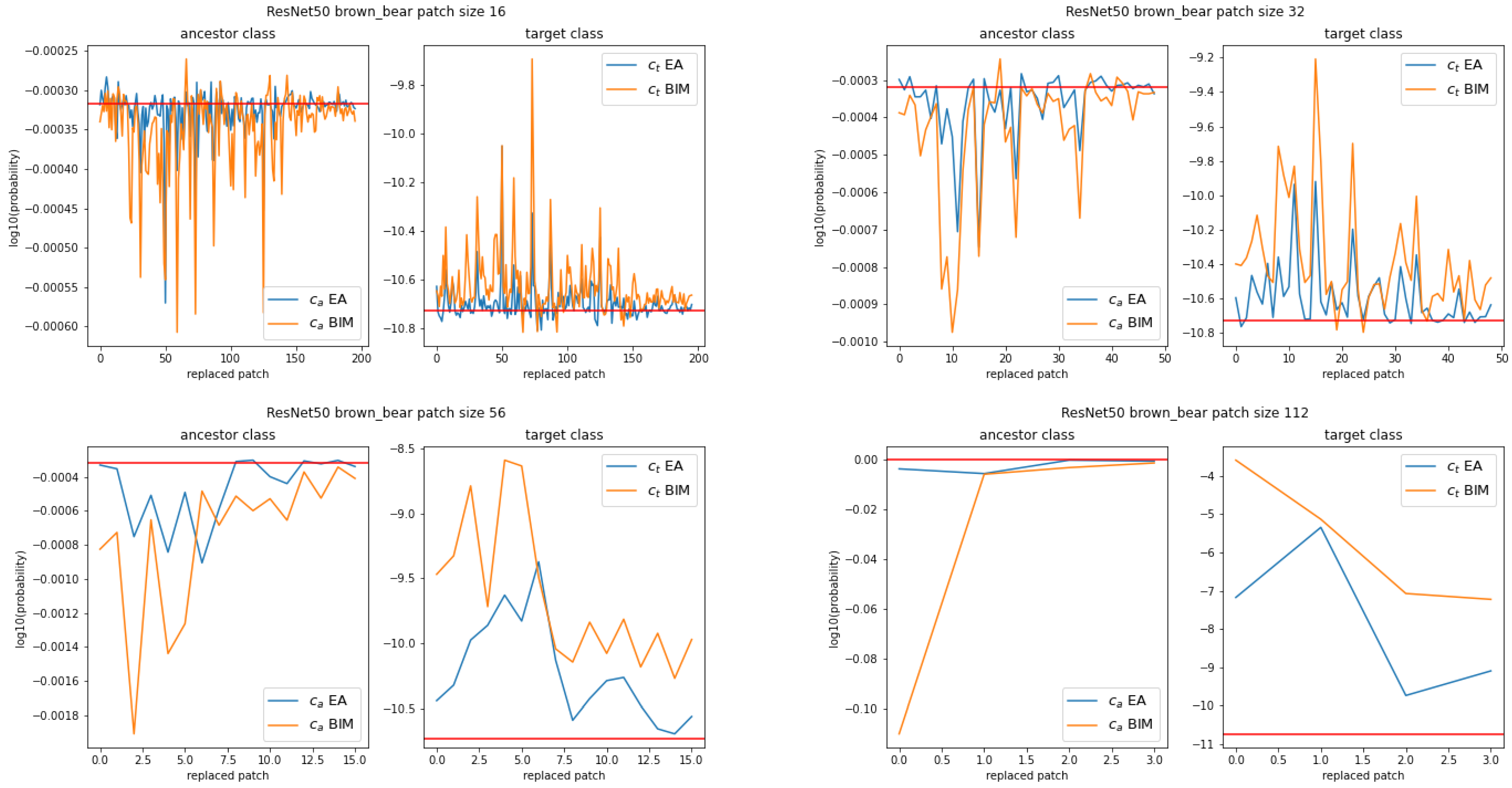Figure 1 shows an example of the plots of these successive $c_a$ and $c_t$-label values, step-by-step, for the ancestor image ${\mathcal{A}}_5^4$, the CNN ${\mathcal{C}}_6$, and the adversarial images obtained by the EA and BIM. The behavior illustrated in this example is representative of what happens for all ancestors and CNNs.

For all values of s and both attacks, almost all patches individually increase the $c_t$-label value and decrease the $c_a$-label value. The fact that the peaks often coincide between the EA and BIM proves that modifying the ancestor in some image areas rather than others can make a large difference. However, BIM’s effect is usually larger than the EA’s. Note also that no single patch is sufficient to fool the CNNs in the sense that it would create a hybrid image with a dominating $c_t$-label value.

3.2. Is the Global Random Aggregation of Local Adversarial Effect Sufficient to Fool the CNNs?

First, replacing all patches simultaneously and at the correct location is, by definition, enough for a targeted misclassification, since its completion leads to the adversarial image. Second, most of the patches taken individually have a local adversarial impact, but none are sufficient to individually achieve a targeted attack.

The issue addressed here is whether the global aggregation of the local adversarial effect is strong enough, independent of the location of the patches, to create the global adversarial effect that we are aiming at.

We proceed as follows. Given an image I and an integer s such that patches of size $s\times s$ create a partition of I, $sh(I,s)$ is a shuffled image deduced from I by randomly swapping all its patches. With these notations, $sh({\mathcal{D}}_k^{atk}({\mathcal{A}}_q^p),s)$ (with $atk=BIM$ or $EA$) is sent to ${\mathcal{C}}_k$ CNN. One obtains the $c_a$ and $c_t$-label values as well as the dominant category (which may differ from $c_a,c_t$). The values of s used in our tests are 16, 32, 56, and 112, leading to partitions of the $224\times 224$ images into 196, 49, 16, and 4 patches, respectively.

Table 2. Percentages of shuffled images $sh({\mathcal{A}}_q^p,s)$ (first percentage), $sh(D_k^{EA}({\mathcal{A}}_q^p),s)$ (second percentage), and $sh(D_k^{BIM}({\mathcal{A}}_q^p),s)$ (third percentage) for which the predicted class is c.

s	Number of Patches	$\mathit{c}={\mathit{c}}_{\mathit{a}}$	$\mathit{c}\notin \{{\mathit{c}}_{\mathit{a}},{\mathit{c}}_{\mathit{t}}\}$	$\mathit{c}={\mathit{c}}_{\mathit{t}}$
16	196	0.4, 0.1, 0.1	99.6, 99.9, 99.9	0.0, 0.0, 0.0
32	49	18.0, 9.2, 5.3	82.0, 90.8, 94.4	0.0, 0.0, 0.3
56	16	67.6, 39.3, 15.8	32.4, 60.3, 70.1	0.0, 0.4, 14.1
112	4	88.4, 62.3, 22.3	11.6, 33.2, 35.9	0.0, 4.5, 41.8

gives the outcome of these tests. For each value s, each cell is composed of a triplet of numbers. The left one corresponds to the tests with the ancestor images, the middle one corresponds to the tests with images obtained by the EA, and the right one corresponds to the tests with images obtained by BIM. Each number is the percentage of images $sh({\mathcal{A}}_q^p,s)$ or of images $sh({\mathcal{D}}_k^{atk}({\mathcal{A}}_q^p),s)$ taken for all ancestor images ${\mathcal{A}}_q^p$, all (ancestor and target) category pairs, and all ${\mathcal{C}}_1,\cdots ,{\mathcal{C}}_{10}$, which are classified in category c, where c is the ancestor category $c_a$, the target category $c_t$, or any other class. To allow for comparisons, the randomly selected swapping order of the patches is performed only once per value of s. For each s, this uniquely defined sequence is applied in the same manner to create the $sh({\mathcal{A}}_q^p,s)$, $sh({\mathcal{D}}_k^{EA}({\mathcal{A}}_q^p),s)$, and $sh({\mathcal{D}}_k^{BIM}({\mathcal{A}}_q^p),s)$ shuffled images.

Contrary to what occurs with $s=32,56$ and 112, the proportion of shuffled ancestors $sh({\mathcal{A}}_q^p,s)$ classified as $c_a$ is negligible for $s=16$. Therefore, $s=16$ seems to lead to patches that are too small for a $224\times 224$ image to allow for a meaningful comparison between the ancestor and adversarials and is consequently disregarded in the remainder of this subsection. At all other values of s, the classification of the shuffled adversarial image as a class different from $c_a$ ($c_t$ or other) is more common with BIM than with the EA. With $s=112$, it is noticeable that as many as 41.8% of BIM shuffled adversarials still produce targeted misclassifications. Enlarging s from 56 to 112 dramatically increases the proportion of shuffled adversarials classified as $c_t$ with BIM (with a modest increase with the EA) and as $c_a$ with the EA (with a modest increase with BIM). Moreover, the shuffled EA adversarials behave similarly to the shuffled ancestors, the $c_a$ probability of which increases considerably as the size of the patches grows larger and the original $c_a$ object becomes clearer (despite its shuffled aspect).

3.3. Summary of the Outcomes

Both the EA and BIM attacks have an adversarial local effect, even at patch sizes as small as $16\times 16$, but they generally require the image to be at full scale in order to be adversarial in the targeted sense. However, the difference between the attacks is that as the patch size increases (without reaching full scale and while being subject to a shuffling process) and the $c_a$ shape consequently becomes more obvious (even despite shuffling), the EA’s noise has a lower adversarial effect, while BIM’s $c_t$-meaningful noise actually accumulates and has a higher global adversarial effect.

4. Adversarial Noise Visualization and Frequency Analysis

This section first attempts to provide a visualization of the noise that the EA and BIM add to an ancestor image to produce an adversarial image (Section 4.1). We then look more thoroughly at the frequencies of the noise introduced by the EA and BIM (Section 4.2). Finally, we look for the frequencies that are key to the adversarial nature of an image created by the ${\mathrm{EA}}^{\mathrm{target},\mathcal{C}}$ and by BIM (Section 4.3).

4.1. Adversarial Noise Visualization

The visualization of the noise that ${\mathrm{EA}}^{\mathrm{target},{\mathcal{C}}_k}$ and BIM add to ${\mathcal{A}}_q^p$ to create the $0.999$-strong adversarial images ${\mathcal{D}}_k^{EA}\left({\mathcal{A}}_q^p\right)$ and ${\mathcal{D}}_k^{BIM}\left({\mathcal{A}}_q^p\right)$ is performed in two steps. First, the difference ${\mathcal{D}}_k^{atk}\left({\mathcal{A}}_q^p\right)-{\mathcal{A}}_q^p$ between each adversarial image and its ancestor is computed for each RGB channel. Second, a histogram of the adversarial noise is displayed. This leads to the measurement of the magnitude of each pixel modification. An example, typical of the general behavior regardless of the channel, is illustrated in Figure 2, showing the noise (the fact that the dominating colors of the noise representation displayed in Figure 2 are green, yellow, and purple stems from the ’viridis’ setting in Python’s matplotlib library, which could be changed at will, but still, the scale gives the amplitude of the noise per pixel in the range $[-ϵ,ϵ]=[-0.03,0.03]$ and hence justifies the position of the observed colors) and histogram of the perturbations added to the red channel of ${\mathcal{A}}_5^4$ to fool ${\mathcal{C}}_6$ with the EA and BIM.

Recall that both attacks perform pixel perturbations with a maximum perturbation magnitude of $ϵ=0.03$ (see Section 2.4). However, with BIM, the smaller magnitudes dominate the histogram and the adversarial noise is closer to a uniform distribution with the EA. Another difference is that, whereas with BIM, all pixels are modified, a considerable number of pixels (9.3% on average) are not modified at all with the EA. Overall, there is a larger variety of noise magnitudes with the EA than with BIM, which can also be observed visually in the image display of the noise.

4.2. Assessment of the Frequencies Present in the Adversarial Noise

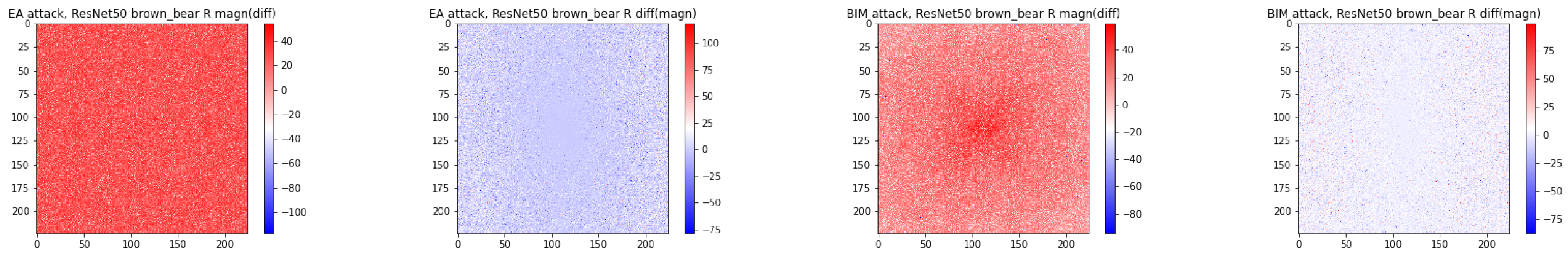
With the adversarial perturbations ${\mathcal{D}}_k^{atk}\left({\mathcal{A}}_q^p\right)-{\mathcal{A}}_q^p$ having been assessed (Section 4.1) for each RGB channel, we proceed to an analysis of the frequencies present in the adversarial noise per channel. Specifically, the Discrete Fourier Transform (DFT) is used to obtain the 2D magnitude spectra of the adversarial perturbations. We compute two quantities: magn (diff) $=|DFT({\mathcal{D}}_k^{atk}({\mathcal{A}}_q^p)-{\mathcal{A}}_q^p)|$, and diff (magn) $=|DFT({\mathcal{D}}_k^{atk}({\mathcal{A}}_q^p))|-|DFT({\mathcal{A}}_q^p)|$. Figure 3 displays a typical example of the general outcome regarding the adversarial noise in the red channel added by the EA or by BIM. For each image, the low frequencies are represented in the center, the high frequencies are represented in the corners, and the vertical bar (on the right) maps the frequency magnitudes to the colors shown in the image.

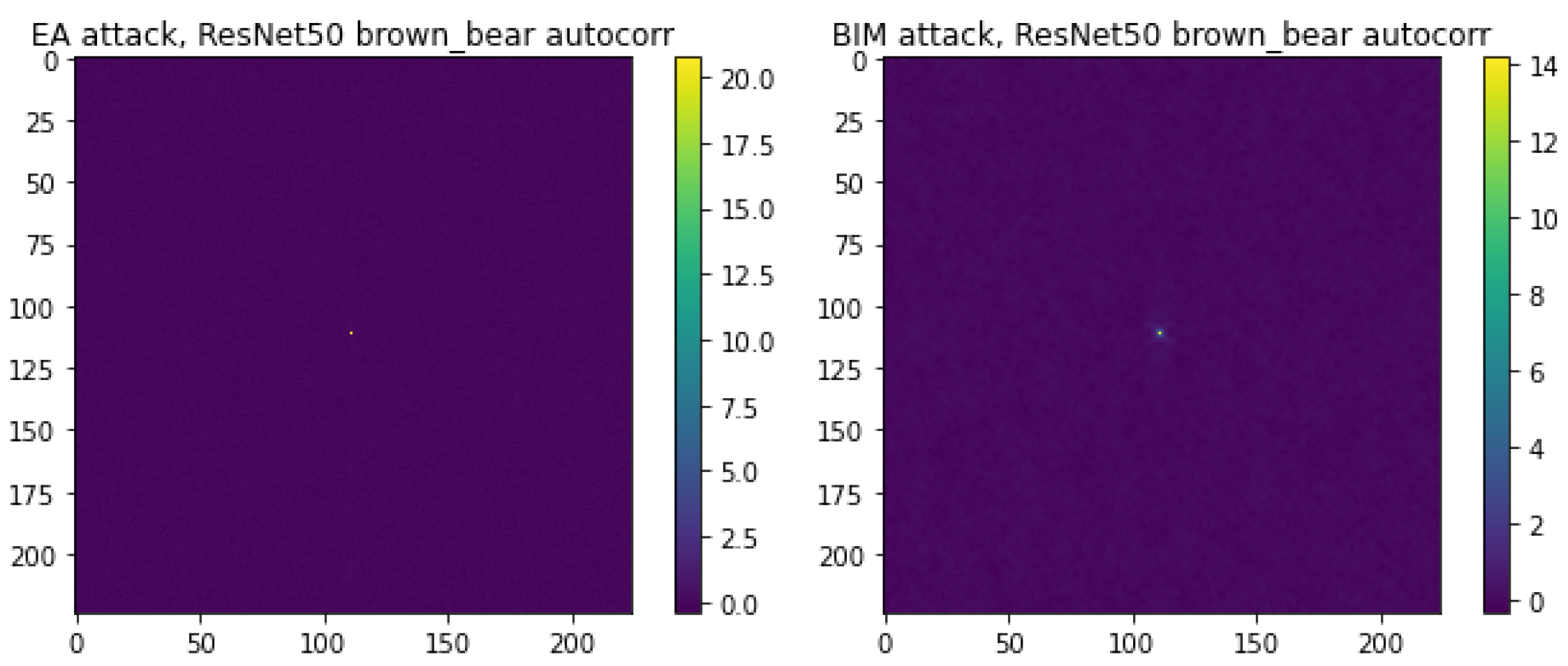
A clear difference between the EA and BIM is visible from the magn (diff) visualizations. With the EA, the high magnitudes do not appear to be concentrated in any part of the spectrum (with the exception of occasional high magnitudes in the center), indicating the white noise nature of the added perturbations. Supporting evidence for the white noise nature of the EA comes from the $2D$ autocorrelation of the noise. Figure 4 shows that the $2D$ autocorrelation for both attacks have a peak at lag 0, which is expected. It turns out that this is the only peak when one considers the EA, which is no longer the case when considering BIM. Unfortunately, this is difficult to see in Figure 4, since the central peak takes very high values; hence, the other peaks fade away in comparison. With BIM, the magn (diff) visualizations display considerably higher magnitudes for the low frequencies, indicating that BIM primarily uses low-frequency noise to create adversarial images.

In the case of diff (magn), both the EA and BIM exhibit larger magnitudes at high frequencies than at low frequencies. This can be interpreted as a larger effect of the adversarial noise on the high frequencies than on the low frequencies. Natural images from ImageNet have significantly more low-frequency than high-frequency information [20]. Therefore, even a quasi-uniform noise (such as the EA’s) has a proportionally larger effect on the components that are numerically less present than on the more numerous ones.

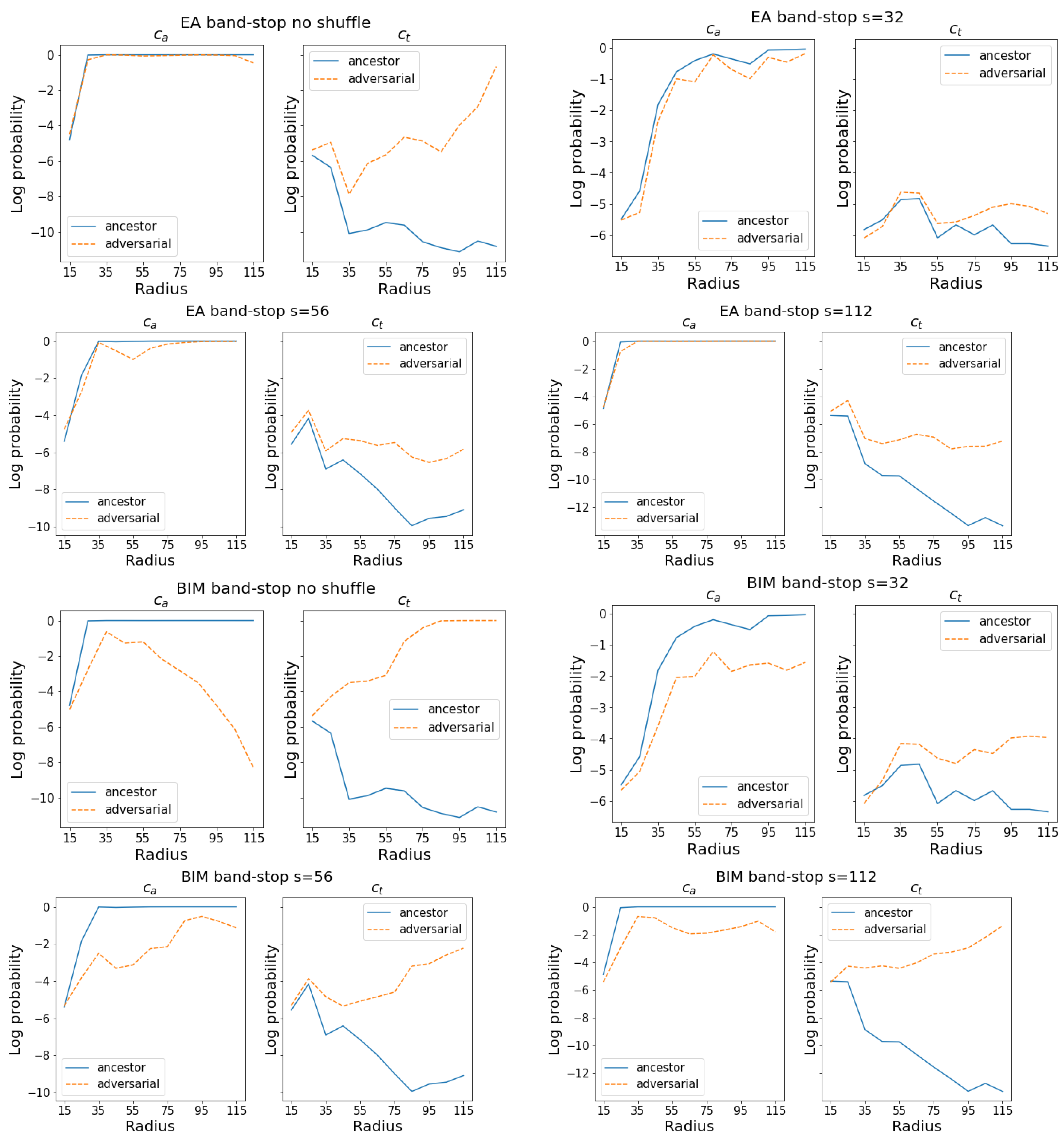
4.3. Band-Stop Filtering Shuffled and Unshuffled Images: Which Frequencies Make an Image Adversarial?

Thus far, the results of this study have revealed the quantity of all frequency components present in the adversarial perturbations, but their relevance to the attack effectiveness is still unknown. To address this issue, we band-stop filter the adversarial images ${\mathcal{D}}_k^{atk}\left({\mathcal{A}}_q^p\right)$ to eliminate various frequency ranges and check the effect produced on the CNN predictions. To evaluate the proportion of low vs. high frequencies of the noise introduced by the two attacks, the process is repeated with the shuffled adversarials $sh({\mathcal{D}}_k^{atk}({\mathcal{A}}_q^p),s)$ for $s=32,56$ and 112.

We first obtain the DFT of all shuffled or unshuffled ancestor and adversarial images, followed by filtering with band-stop filters of 10 different frequency ranges $F_{bst,rc}$, where the range center $rc$ goes from 15 to 115 units per pixel, with steps of 10, and the bandwidth $bw$ is fixed to 30 units per pixel. For example, the last band-stop filter $F_{bst,115}$ removes frequencies in the range of $(115-15,115+15)$ units per pixel. The band-stopped images are passed through the Inverse DFT (IDFT) and sent to the CNN, which results in 10 pairs of $(c_a,c_t)$-label values for each image, be it an ancestor or an adversarial. Figure 5 presents some results that are typical of the general behavior.

For both the EA and BIM, the $c_t$ probability tends to increase as $rc$ increases. This means that lower frequencies have a larger impact on the adversarial classification than higher frequencies. As shown in the left column of each pair of graphs, it is the low frequencies that matter for the correct classification of the ancestor, as well. Although with both attacks, the $c_t$ probability tends to increase at higher values of $rc$, with BIM, it is dominant at considerably smaller values of $rc$, whereas the EA adversarials are usually still classified as $c_a$. Hence, the EA adversarials require almost the full spectrum of perturbations to fool the CNNs, whereas the lower part of the spectrum is sufficient for BIM adversarials. This result matches those of magn (diff) in Figure 3, where the EA and BIM were found to introduce white and predominantly low-frequency noise, respectively.

As for the shuffled images, it is clear that their low-frequency features are affected by the shuffling process, and as a result, the $c_t$ probability cannot increase to the extent it does in the unshuffled images. With BIM and $s=112$, at high rcs, the band-stop graphs show a slower increase in the $c_t$ probability than when the images are not shuffled. This implies that a large part of the BIM adversarial image’s low-frequency noise is meaningful only for the unshuffled image. When this low-frequency noise changes location through the shuffling process, one needs to gather noise across a broader bandwidth to significantly increase the $c_t$ probability of the shuffled adversarial.

Even if the BIM adversarials require a larger bandwidth to be adversarial when shuffled, they still reach this goal. In contrast, the shuffled EA adversarials have band-stop graphs that closely resemble the shuffled ancestors’ graph. Only BIM’s remaining low and middle frequencies are meaningful enough to $c_t$ and still manage to increase the $c_t$ probability.

4.4. Summary of the Outcomes

The histogram of the adversarial noise introduced by BIM follows a bell shape (hence smaller magnitudes dominate), while it is closer to a uniform distribution with the EA (hence with a larger variety of noise magnitudes in this case). In addition, BIM modifies all pixels, while the EA leaves many (approximately 14,000 out of $224\times 224\times 3$, hence 9.3% on average) unchanged.

In terms of the frequency of the adversarial noise, the EA introduces white noise (meaning that all possible frequencies occur with equal magnitude), while BIM introduces predominantly low-frequency noise. Although for both attacks, the lower frequencies have the highest adversarial impact, the low and middle frequencies are considerably more effective with BIM than with the EA.

5. Transferability and Texture Bias

This section examines whether adversarial images are specific to their targeted CNN or whether they contain rather general features that are perceivable by other CNNs (Section 5.1). Since ImageNet-trained CNNs are biased towards texture [21], it is natural to ask whether adversarial attacks take advantage of this property. More precisely, we examine whether texture is changed by the EA and BIM and whether this could be the common “feature” perceived by all CNNs (Section 5.2). Using heatmaps, we evaluate whether CNNs with differing amounts of texture bias agree on which image modifications have the largest adversarial impact and whether texture bias plays any role in transferability (Section 5.3).

5.1. Transferability of Adversarial Images between the 10 CNNs

For each attack $atk\in \{EA,BIM\}$, we check the transferability of the adversarial images as follows. Starting from an ancestor image ${\mathcal{A}}_q^p$, we input the ${\mathcal{D}}_k^{atk}\left({\mathcal{A}}_q^p\right)$ image, which is adversarial against ${\mathcal{C}}_k$, to a different ${\mathcal{C}}_i$ (hence, $i\ne k$). We then extract the probability of the dominant category, the $c_t$ probability, and the $c_a$ probability given by ${\mathcal{C}}_i$ for that image.

Then, we check whether the predicted class is precisely $c_t$ (targeted transferability) or if it is any other class different from both $c_a$ and $c_t$. Out of all possible CNN pairs, our experiments showed that none of the adversarial images created by the EA for one CNN are classified by another as $c_t$, while this phenomenon occurs for 5.4% of the adversarial images created by BIM. As for classification in a category $c\ne c_a,c_t$, the percentages are 5.5% and 3.2% for the EA and BIM, respectively.

5.2. How Does CNNs’ Texture Bias Influence Transferability?

Knowing that CNNs trained on ImageNet are biased towards texture, we assume that a high probability for a particular class given by such a CNN expresses the fact that the input image contains more of that class’s texture. Our goal is to check whether this occurs for adversarial images as well.

We restrict our study to adversarial images obtained by the EA and BIM for the following three CNNs, which have a similar architecture and have been proven [24] to gradually have less texture bias and less reliance on their texture-encoding neurons: $T_1=$ BagNet-17 [33], $T_2=$ ResNet-50, and $T_3=$ ResNet-50-SIN [21]. The experiments amount to checking the transferability of the adversarial images between these three CNNs. The fact that the statement about the graduation is fully proven only for these three justifies that we limit our study to them, since no such hierarchy is known for other CNNs in general.

Even in this case of three CNNs with similar architectures, the experiments show that targeted transferability between the three CNNs is 0%, regardless of the attack. Consequently, checking whether $c_t$ becomes dominant for another CNN is unnecessary. Instead, we calculate the difference produced in a CNN’s predictions of the $c_t$ and $c_a$ probabilities between the ancestor and another CNN’s adversarial image. The average results over all images are presented in

Table 3. The images, adversarial for the CNNs of the rows, are fed to the CNNs of the columns to obtain their $c_a$ and $c_t$ label values. In each cell of the table are the average differences in the $c_a$ and $c_t$ label values between the adversarial ${\mathcal{D}}_{T_t}^{atk}\left({\mathcal{A}}_q^p\right)$ and the ancestor ${\mathcal{A}}_q^p$.

	${\mathit{c}}_{\mathit{a}}$						${\mathit{c}}_{\mathit{t}}$
	${\mathit{T}}_{\mathbf{1}}$		${\mathit{T}}_{\mathbf{2}}$		${\mathit{T}}_{\mathbf{3}}$		${\mathit{T}}_{\mathbf{1}}$		${\mathit{T}}_{\mathbf{2}}$		${\mathit{T}}_{\mathbf{3}}$
atk	EA	BIM	EA	BIM	EA	BIM	EA	BIM	EA	BIM	EA	BIM
$T_1$			−0.03	−0.05	0.01	0.02			$5.6\times {10}^{-5}$	$2.0\times {10}^{-5}$	$1.0\times {10}^{-5}$	$4.1\times {10}^{-5}$
$T_2$	−0.15	−0.22			$1.9\times {10}^{-3}$	−0.01	$2.9\times {10}^{-4}$	$1.1\times {10}^{-3}$			$5.0\times {10}^{-5}$	$1.2\times {10}^{-4}$
$T_3$	−0.15	−0.15	−0.05	−0.13			$2.4\times {10}^{-4}$	$6.8\times {10}^{-5}$	$5.3\times {10}^{-5}$	$5.7\times {10}^{-4}$

.

When transferring from $T_2=$ ResNet-50 to $T_1=$ BagNet-17, the experiments show that the $c_a$-label value decreases while the $c_t$-label value increases, with the former being larger in magnitude than the latter. If the assumption formulated in the first paragraph holds, this phenomenon implies that the attacks change image texture. However, the similarly low transferability from $T_1=$ BagNet-17 to $T_2=$ ResNet-50 proves that texture change is not sufficient to generate adversarial images. The texture change observed in $T_2=$ ResNet-50 adversarials might simply be a side effect of the perturbations created by the EA and BIM.

Nevertheless, Table 3 reveals that texture bias seems to play a role in transferability. It shows that the more texture-biased the CNN that the adversarial images are transferred to, the larger the decrease in its $c_a$-label values. Indeed, this $c_a$ decrease is larger when transferring from $T_3=$ ResNet-50-SIN to $T_2=$ ResNet-50 and from $T_2=$ ResNet-50 to $T_1=$ BagNet-17 than vice-versa.

5.3. How Does Texture Change Relate to Adversarial Impact on the CNNs?

In this subsection, BagNet-17 is used to visualize, thanks to heatmaps, whether texture change correlates with the adversarial impact of the obtained images for the 10 CNNs ${\mathcal{C}}_1,\cdots ,{\mathcal{C}}_{10}$.

Although we have seen that both attacks affect BagNet-17’s $c_a$ probability on average, here, we attempt to find the image areas in which these changes are most prominent and to compare the locations in the ${\mathcal{C}}_k$ adversarials that have the largest impact on BagNet-17 and on ${\mathcal{C}}_k$.

To achieve this, we proceed in a similar manner as in Section 3.1, with the difference that we allow overlaps. We replace all overlapping $17\times 17$ patches of the ancestor ${\mathcal{A}}_q^p$ with patches from the same location in ${\mathcal{D}}_k^{atk}\left({\mathcal{A}}_q^p\right)$, a single patch at a time, and we extract and store the $c_a$ and $c_t$ probabilities given by ${\mathcal{C}}_k$ of the obtained hybrid image I at each step. Contrary to the situation in Section 3.1, note that there are as many patches as pixels in this case. Simultaneously, these patches are also fed to BagNet-17 (leading to 50,176 predictions for each adversarial image) to extract the $c_a$ and $c_t$-label values of these patches. The stored $c_a$ and $c_t$ label values (and combinations of them) can be displayed in a square box of size $224\times 224$ (hence of sizes equal to the size of the handled images), resulting in a heatmap.

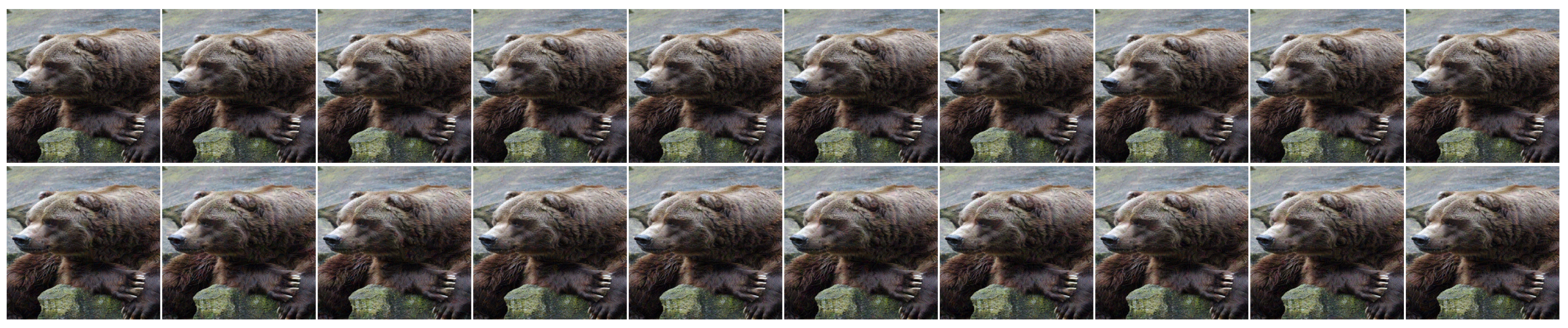
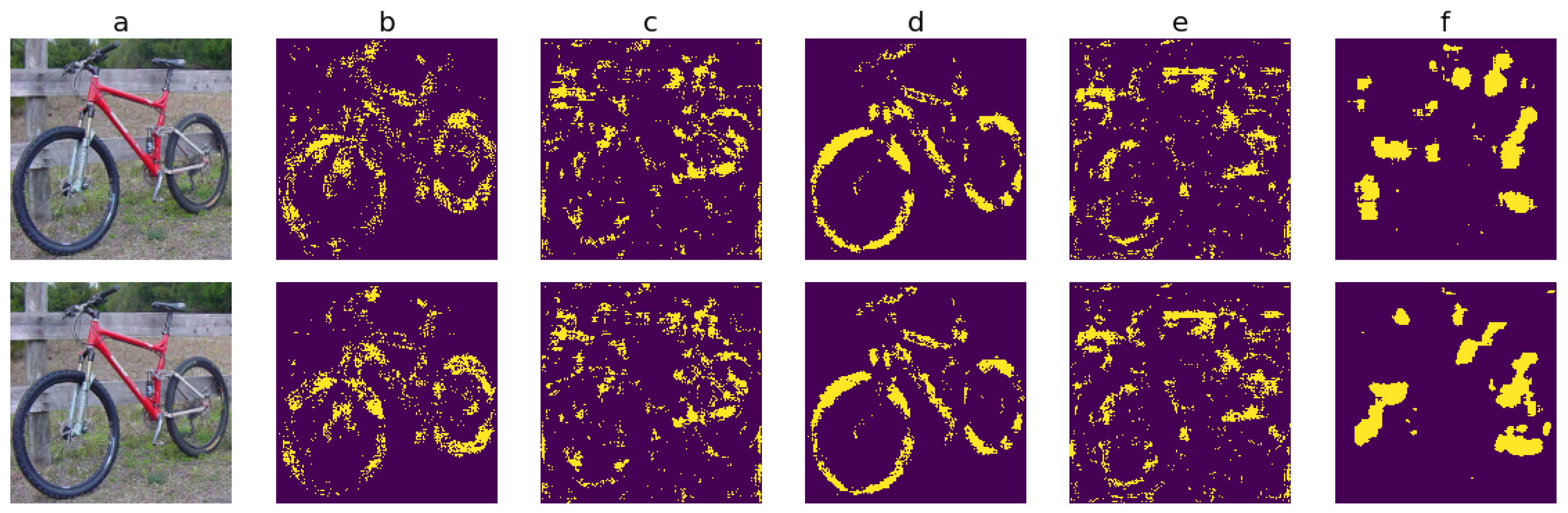
More precisely, given an ancestor image ${\mathcal{A}}_q^p$, all hybrid adversarial images obtained as above via the EA lead to 5 heatmaps, and all those obtained by BIM lead to 5 heatmaps as well. For both attacks, the first four heatmaps are obtained using BagNet-17, and the fifth is obtained using ${\mathcal{C}}_k$ for comparison purposes. Each heatmap assesses the 10% largest variations in the following sense.

We have the first sequence ${\left(c_a\left(P\left(\mathcal{D}\left(\mathcal{A}\right)\right)\right)\right)}_P$ of $c_a$-label values obtained from the evaluation by BagNet-17 of the patches of the adversarial images and a second similar sequence ${\left(c_a\left(P\left(\mathcal{A}\right)\right)\right)}_P$ of $c_a$-label values coming from the patches of the ancestor images. Both sequences are naturally indexed by the same successive patch locations P. We then consider that the sequence, also indexed by the patches, was made up of the differences $c_a\left(P\left(\mathcal{D}\left(\mathcal{A}\right)\right)\right)-c_a\left(P\left(\mathcal{A}\right)\right)$. The selection of locations of the smallest 10% out of this sequence of differences leads to the first heatmap. One proceeds similarly for the second heatmap by selecting the location of the largest 10% of the values of $c_t\left(P\left(\mathcal{D}\left(\mathcal{A}\right)\right)\right)-c_t\left(P\left(\mathcal{A}\right)\right)$ (with obvious notations). The process is similar for the third and fourth heatmaps, where one considers the location of the largest 10% of the values of $c_a\left(P\left(\mathcal{D}\left(\mathcal{A}\right)\right)\right)-c_t\left(P\left(\mathcal{D}\left(\mathcal{A}\right)\right)\right)$ for the third heatmap and of the values of $c_t\left(P\left(\mathcal{D}\left(\mathcal{A}\right)\right)\right)-c_a\left(P\left(\mathcal{D}\left(\mathcal{A}\right)\right)\right)$ for the fourth heatmap.

Finally, the fifth heatmap is obtained by considering the largest 10% of the values $c_t(I_{P(\mathcal{D}(\mathcal{A}))})-c_t(\mathcal{A})$, where the two members of the difference are the $c_t$-label values given by the CNN ${\mathcal{C}}_k$ for a full image: the right one for the ancestor image and the left one for the hybrid image, obtained as explained above.

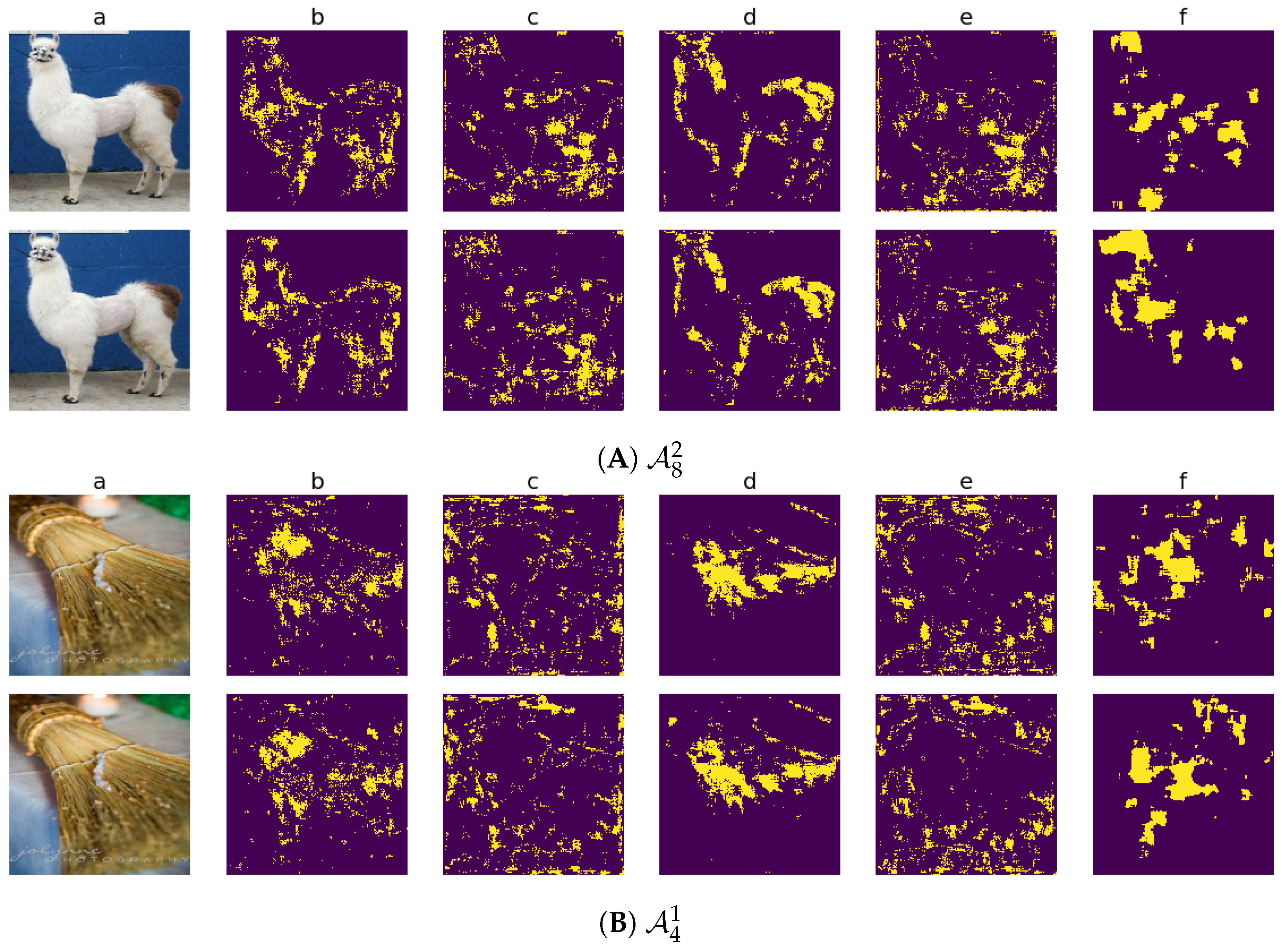
Figure 6 shows the outcome of this process for ${\mathcal{C}}_6$ = ResNet-50 and ancestor ${\mathcal{A}}_{10}^8$ (see Figure A5 in Appendix B.1 for other examples). Figure 6a shows the adversarial images ${\mathcal{D}}_6^{EA}({\mathcal{A}}_{10}^8)$ (top) and ${\mathcal{D}}_6^{BIM}({\mathcal{A}}_{10}^8)$ (bottom). Figure 6b–e are the four heatmaps obtained thanks to BagNet-17 (in the order stated above), and Figure 6f is the heatmap obtained thanks to ${\mathcal{C}}_6$ (the top row corresponds to the EA, and the bottom row corresponds to BIM). The 10% largest variations are represented by yellow points in each heatmap.

With both attacks, actually stronger with BIM than with the EA, modifying the images in and around the object locations is the most effective at increasing ${\mathcal{C}}_k$’s $c_t$ probability, as shown in Figure 6f.

For both attacks, the locations where the $c_a$ texture decreases coincide with the locations of most adversarial impact for ${\mathcal{C}}_k$ (Figure 6b,f), while the $c_t$ texture increase is slightly more disorganized, being distributed across more image areas (Figure 6c). However, even though the $c_a$ texture decreases, it remains dominant in the areas where the $c_a$ shape is also present (Figure 6d), without being replaced by the $c_t$ texture, which only dominates in other, less $c_a$ object-related areas (Figure 6e). The $c_a$ texture and shape coupling encourages the classification of the image into $c_a$, which may explain why the adversarial images are not transferable.

5.4. Summary of the Outcomes

Both attacks’ adversarial images are generally not transferable in the targeted sense. Although some $c_a$ texture is distorted by the attacks, the $c_t$ texture is not significantly increased (while the opposite is true for the targeted CNNs’ $c_a$ and $c_t$ probabilities), and this increase is nevertheless not correlated with an adversarial impact on the CNNs. However, we find that the EA’s and BIM’s adversarial images transfer more to CNNs, which have higher texture bias.

6. Transferability of the Adversarial Noise at Smaller Image Regions

On the one hand, the very low transferability rate observed in Section 5 shows that most obtained adversarial images are specific to the CNNs they fool. On the other hand, the size of the covered region increases linearly with successive CNN layers [36]. Moreover, the similarity between the features captured by different CNNs is higher in earlier layers than in later layers [37,38]. Roughly speaking, the earlier layers tend to capture information of a general nature, common to all CNNs, whereas the features captured by the later layers diverge from one CNN to another.

The question addressed in this section goes in the direction of a potential stratification of the adversarial noise’s impact according to the successive layers of the CNNs. In other words, this amounts to clarifying whether it is possible to sieve the adversarial noise, so that one would identify the part of the noise (if any) that has an adversarial impact for all CNNs up to some layers, and the part of the noise in which adversarial impact becomes CNN-specific from some layer on. This is a difficult challenge since the adversarial noise is modified continuously until a convenient adversarial image is created. In particular, the “initial” noise, created at some early point of the process and potentially adversarial for the first layers of different CNNs, is likely to be modified as well during this process, and to lose its initial “quasi-universal” adversarial characteristic, potentially to the benefit of a new adversarial noise. Note en passant that a careful study in this direction may contribute to “reverse engineer” a CNN, namely to reconstruct its architecture (up to a point). This direction is only indicated here and is not explored in full details at this stage.

More modestly and more specifically, in this section, we ask whether the adversarial noise for regions of smaller sizes is less CNN-specific and, hence, more transferable than at full scale, namely $224\times 224$ in the present case, where we know that, in general, it is not transferable.

This issue is addressed in two ways. First, we check whether and how a modification of the adversarial noise intensity affects the $c_a$ and the $c_t$-label values of an image, adversarial for a given CNN, when exposed to a different CNN, and the influence of shuffling in this process (Section 6.1). Second, we keep the adversarial noise as it is, and we check whether adversarial images are more likely to transfer when they are shuffled (Section 6.2).

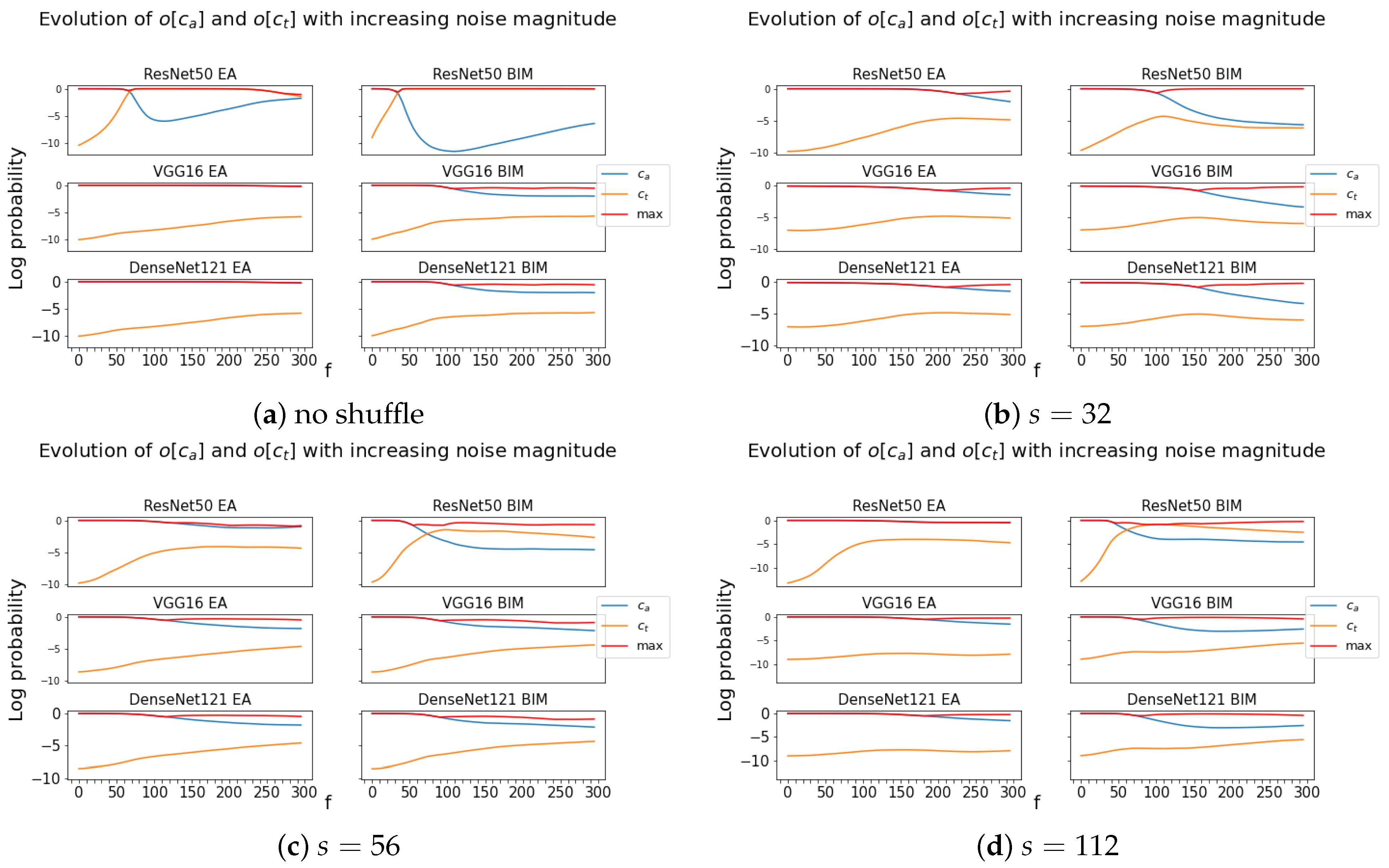
6.1. Generic versus Specific Direction of the Adversarial Noise

One is given a convenient ancestor image ${\mathcal{A}}_q^p$, a CNN ${\mathcal{C}}_k$, and the adversarial images ${\mathcal{D}}_k^{EA}\left({\mathcal{A}}_q^p\right)$ and ${\mathcal{D}}_k^{BIM}\left({\mathcal{A}}_q^p\right)$ obtained by both attacks.

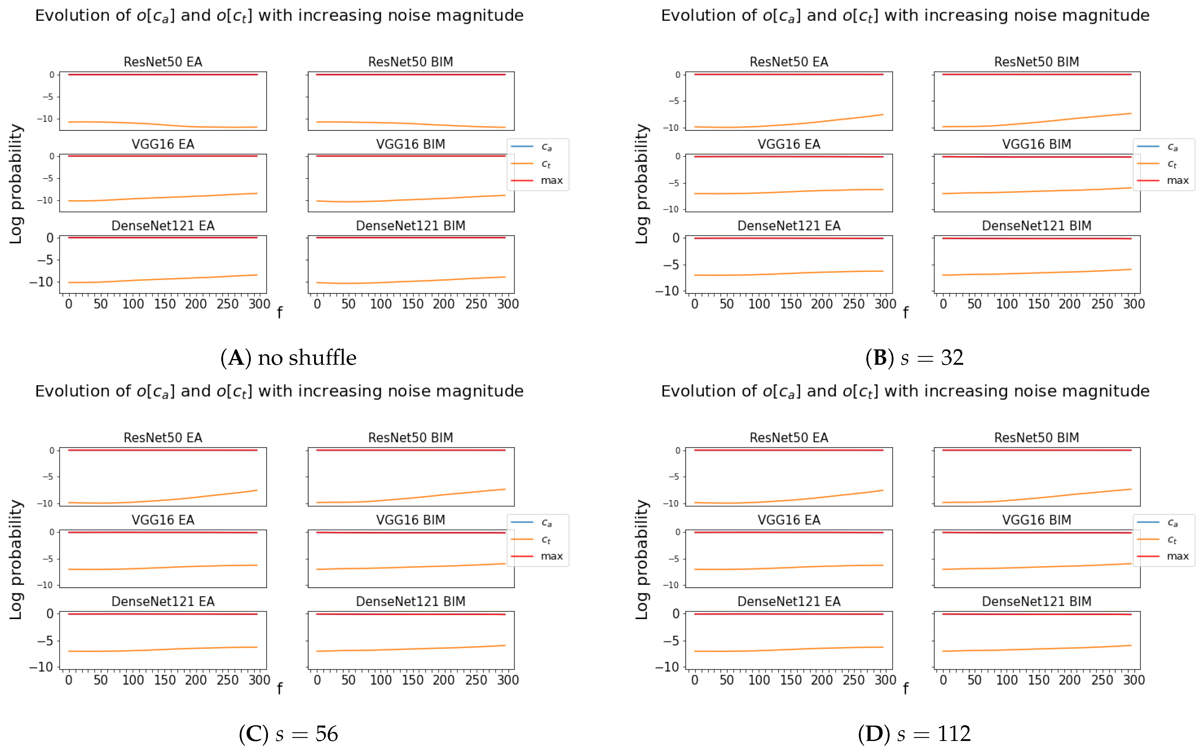
We perform the first series of experiments, which consists of changing the adversarial noise magnitude of these adversarial images by a factor f in the 0–300% range and of submitting the corresponding modified f-boosted adversarial images to different ${\mathcal{C}}_i$s to check whether they fool them.

Figure 7a shows what happens for the particular case of ${\mathcal{A}}_5^4$, $k=6$, and to the ${\mathcal{C}}_i$s equal to ${\mathcal{C}}_1,{\mathcal{C}}_6$, and ${\mathcal{C}}_9$ (the f-boosted adversarial image is sent back to ${\mathcal{C}}_6$ as well), representative of the general behavior. In particular, it shows that the direction of the noise created for the EA adversarials is highly specific to the targeted CNN since the images cannot be made transferable by any change in magnitude. A contrario, the noise of BIM’s adversarials has a more general direction, since amplifying its magnitude eventually leads to untargeted misclassifications by other CNNs.

A second series of experiments is performed in a similar manner as above, with the difference that, this time, it is on the shuffled adversarial images $sh({\mathcal{D}}_k^{EA}({\mathcal{A}}_q^p),s)$ and $sh({\mathcal{D}}_k^{BIM}({\mathcal{A}}_q^p),s)$ for $s=32$, 56, or 112.

Figure 7b–d show the typical outcome of this experiment. It reveals another difference between the adversarial noise obtained by the two attacks, namely, when s is increased from 32 to 56 and 112, BIM images have a higher adversarial effect on other CNNs, whereas the EA images only have a higher adversarial effect when s is increased from 32 to 56. As the size of the shuffled boxes increases to $s=112$ and reveals the ancestor object more clearly, the EA adversarials actually have a lower fooling effect on other CNNs.

Moreover, in contrast to Figure 7a, where the considered region is at full scale, i.e., coincides with the full image size, Figure 7b–d show that the noise direction is more general at the local level and that an amplification of the noise magnitude is able to lead the adversarial images outside of other CNNs’ $c_a$ bounds, even with the EA.

To ensure that the observed effects were not simply due to shuffling but were also due to the adversarial noise, we repeated the experiment shown in Figure 7 with random normal noise. As expected, it turned out that, with random noise, the $c_a$-label value always remained dominant and the $c_t$-label value barely increased as f varied from 0% to 300% (see Figure A6 in Appendix B.2). The close-to-zero impact of random noise on unshuffled images was already known [39]. These experiments confirm that this also holds true for shuffled images. Therefore, the observed effects were indeed due to the adversarial noise’s transferability at the local level. Nevertheless, although the adversarial noise is general enough to affect other CNNs’ $c_a$-label values, its effect on $c_t$-label values is never as strong as for the targeted CNN.

6.2. Effects of Shuffling on Adversarial Images’ Transferability

Here, we do not change the intensity of the noise. That is, $f=100\%$. The point is no longer to visualize the graph of the evolution of the $c_t$-label values of shuffled adversarials but to focus on their actual values for the “real” noise (at $f=100\%$). The issue is to check whether the adversarial images are more likely to transfer when they are shuffled.

We proceed as follows. We input the unshuffled ancestor ${\mathcal{A}}_q^p$ and the unshuffled adversarial ${\mathcal{D}}_k^{atk}\left({\mathcal{A}}_q^p\right)$ to all ${\mathcal{C}}_i$’s for $i\ne k$ (hence, all CNNs except the targeted one). We extract the $c_a$ and $c_t$-label values for each i, namely $c_a^i({\mathcal{A}}_q^p)$, $c_a^i({\mathcal{D}}_k^{atk}({\mathcal{A}}_q^p))$, $c_t^i({\mathcal{A}}_q^p)$, and $c_t^i({\mathcal{D}}_k^{atk}({\mathcal{A}}_q^p))$. We compute the difference in the $c_a$-label values between the two images for each i and, similarly, the difference in the $c_t$-label values to obtain

$${\Delta }_a^{k,i}\left({\mathcal{A}}_q^p\right)=c_a^i({\mathcal{D}}_k^{atk}\left({\mathcal{A}}_q^p\right))-c_a^i\left({\mathcal{A}}_q^p\right),{\Delta }_t^{k,i}\left({\mathcal{A}}_q^p\right)=c_t^i({\mathcal{D}}_k^{atk}\left({\mathcal{A}}_q^p\right))-c_t^i\left({\mathcal{A}}_q^p\right).$$

For $s=32,56$ and 112, this process is repeated with the shuffled ancestor $sh({\mathcal{A}}_q^p,s)$ and the shuffled adversarial $sh({\mathcal{D}}_k^{atk}({\mathcal{A}}_q^p),s)$, yielding the following differences:

$${\Delta }_a^{k,i}(sh({\mathcal{A}}_q^p,s))=c_a^i(sh({\mathcal{D}}_k^{atk}({\mathcal{A}}_q^p),s))-c_a^i(sh({\mathcal{A}}_q^p,s)),$$

and

$${\Delta }_t^{k,i}(sh({\mathcal{D}}_k^{atk}({\mathcal{A}}_q^p),s))=c_t^i(sh({\mathcal{D}}_k^{atk}({\mathcal{A}}_q^p),s))-c_t^i(sh({\mathcal{A}}_q^p),s).$$

These ${\Delta }^{k,i}$ assess the impact of the adversarial noise both when unshuffled and shuffled.

Regarding the $c_a$-label values, both differences are ≤0 (the $c_a$-label value of the ancestor dominates the $c_a$-label value of the adversarial, shuffled or not). We consider the absolute value of both quantities (k and i are fixed). Finally, we compute the percentage over all k, all $i\ne k$, of all convenient ancestors ${\mathcal{A}}_q^p$ for which

$$|{\Delta }_a^{k,i}\left(sh({\mathcal{A}}_q^p,s)\right)|\ge |{\Delta }_a^{k,i}\left({\mathcal{A}}_q^p\right)|.$$

Regarding the $c_t$-label values, both differences are $\ge 0$ (this is obvious for the unshuffled images and turns out to be the case for the shuffled one). In this case, there is therefore no need to take the absolute values. We compute the percentage over all k, all $i\ne k$, of all convenient ancestors ${\mathcal{A}}_q^p$ for which

$${\Delta }_t^{k,i}\left(sh({\mathcal{A}}_q^p,s)\right)\ge {\Delta }_t^{k,i}\left({\mathcal{A}}_q^p\right).$$

Table 4. For the $c_a$-label value (second row) and the $c_t$-label value (third row), the percentage of cases where the adversarial noise has a stronger impact when shuffled than unshuffled. In each cell, the first percentage corresponds to $atk=EA$, and the second corresponds to $atk=BIM$.

	$\mathit{s}=32$	$\mathit{s}=56$	$\mathit{s}=112$
$|{\Delta }_a^{k,i}(sh({\mathcal{A}}_q^p,s))|\ge |{\Delta }_a^{k,i}({\mathcal{A}}_q^p)|$	52.02, 45.41	66.94, 64.29	57.58, 54.67
${\Delta }_t^{k,i}(sh({\mathcal{A}}_q^p,s))\ge {\Delta }_t^{k,i}({\mathcal{A}}_q^p)$	52.69, 49.79	65.09, 58.37	48.24, 43.11

presents the outcome of these computations for each value of s and for the adversarials obtained by both attacks.

Note that we do not simply present the $c_t$-label values of shuffled adversarial images because, then, the measured impact could have two sources: either the adversarial noise or the fact that the $c_a$ shape is distorted by shuffling, leaving room for the $c_t$-label value to increase. Since our goal is to only measure the former source, we compare the $c_t$-label values of shuffled adversarials with those of shuffled ancestors.

When the percentage is larger than 50%, the adversarial images have, on average, a stronger adversarial effect (for the untargeted scenario if one considers ${\Delta }_a^{k,i}$ and for the target scenario if one considers ${\Delta }_t^{k,i}$) when shuffled than when they are not. The adversarial effect is then perceived more by other CNNs for regions of the corresponding same size than at full scale.

For all values of s, the first percentage is larger than the second one. This means that distorting the shape of the ancestor object (done by shuffling) helps the EA more than BIM in fooling other CNNs than the targeted ${\mathcal{C}}_k$. This occurs although computation shows that shuffled BIM adversarials are typically classified with a larger $c_t$-label value than the shuffled EA adversarials.

The percentages achieved with $s=56$ not only are the largest compared with those with $s=32$ or 112 but also exceed 50% by far. Said otherwise, a region size of $56\times 56$ achieves some optimum here. An interpretation could be that a region of that size is small enough to distort the $c_a$-related information more while also being large enough to enable the adversarial pixel perturbations to join forces and to create adversarial features with a larger impact on different CNNs than the targeted one.

6.3. Summary of the Outcomes

The direction of the created adversarial noise for the EA adversarials is very specific to the targeted CNN. No change in magnitude of the adversarial noise makes them more transferable. The situation differs to some extent from the noise of BIM’s adversarials. This latter noise has a more general direction, since its amplification leads to untargeted misclassifications by other CNNs. When images are shuffled and the noise is intensified, BIM’s adversarials have a higher adversarial effect on other CNNs as s grows. This is also the case with the EA’s adversarials as s grows from 32 to 56, but no longer when s increases from 56 to 112.

The second outcome is that the EA and BIM adversarial images become closer to being transferable in a targeted sense when shuffled with $s=56$ than when unshuffled (at their full scale) and that $s=56$ is optimal in this regard compared with $s=32$ or 112. In the untargeted sense, this happens at regions with sizes of $56\times 56$ and $112\times 112$ (for both attacks, the corresponding percentages exceed 50%).

7. Penultimate Layer Activations with Adversarial Images

In this section, we closely examine (in Section 7.2) the changes that adversarial images produce in the activation of the CNNs’ penultimate layers (for reasons explained in Section 7.1). In the work that led to this study, we performed a similar study on the activation changes of the CNNs’ convolutional layers. However, different from what happens with the penultimate layers, the results obtained with adversarial noise were identical to those obtained with random noise. Hence, visualizing the intermediate layer activations requires a more in-depth method than the one employed here and we restrict the current paper to the study of the penultimate classification layers.

It is important to note that we do not pay attention to the black-box or white-box nature of the attack. We use the adversarial images independently on how they are obtained. Indeed, we assume full access to the architectures of the CNNs. This full access to the CNNs’ architectures goes without saying when one considers BIM, since it is a prerequisite for this attack. However, it is worthwhile to explicitly state for the EA, since the EA attack excludes any a priori knowledge of the CNNs’ architectures.

Still, the study of the way layers are activated by the adversarial images may reveal differences in their behaviors according to the methods used to construct them. It is not excluded that the patterns of layer activations differ according to the white-box or black-box nature of the attack that created the adversarial images sent to the CNNs. Should this be the case, this difference in patterns according to the nature of the attack may lead to attack detection or even protection measures. The issue is not addressed in this study.

7.1. Relevance of Analyzing the Activation of $c_t$- and of $c_a$-Related Units

The features extracted by the convolutional CNN layers pass through the next group of CNN layers, namely the classification layers. We focus on the penultimate classification layer, i.e., the layer just before the last one that gives the output classification vector.

When a CNN $\mathcal{C}$ is exposed to an adversarial image $\mathcal{D}\left(\mathcal{A}\right)$, the perturbation of the features propagates and modifies the activation of the classification layers, which in turn leads to an output vector $o_{\mathcal{D}\left(\mathcal{A}\right)}^{\mathcal{C}}$ (drastically different from the output vector $o_{\mathcal{A}}^{\mathcal{C}}$ for the ancestor) in which the probability corresponding to the target class $c_t$ is dominant. To achieve this result, it is certain that previous classification layers are modified in a meaningful manner, with higher activations of the units that are relevant to $c_t$.

However, it is not clear how the changes in these classification layers occur. Since the penultimate layer has a direct connection with the final layer and the impact of changes in activation are thus traceable, we delve into the activations of the CNNs’ penultimate layers to answer two questions essentially: Do all $c_t$-relevant units have increased activation? Do $c_a$-related units have decreased activations?

The connection between the penultimate and final layers is made through a weight vector W, which, for each class in the output vector, provides the weights by which to multiply the penultimate layer’s activation values. Whenever a weight that connects one penultimate layer unit with one class is positive, that particular unit of the penultimate layer is indicative of that class’ presence in the image, and vice-versa for negative weights. We can thus determine which penultimate layer units are $c_a$- or $c_t$-related.

7.2. How Are the CNNs’ Classification Layers Affected by Adversarial Images?

For each CNN ${\mathcal{C}}_k$, we obtain the following. The aforementioned weights are extracted, and for both $c_a$ and $c_t$, they are separated into positive and negative weights. Then, we compute the difference in activation values in the penultimate layer between each adversarial ${\mathcal{D}}_k^{atk}\left({\mathcal{A}}_q^p\right)$ and its ancestor ${\mathcal{A}}_q^p$. Since our intention is to measure the proportion of units, relevant to a class, that are increased or decreased by the adversarial noise, we compute the average percentage of both positively and negatively related units—

Table 5. For $c_a$, average percentage of both positively related ($W_{pos}$, columns 2–4) and negatively related ($W_{neg}$, columns 5–7) units, in which the activation increased (${\Delta }_{pos}$), stagnated (${\Delta }_0$), or decreased (${\Delta }_{neg}$).

	For ${\mathit{c}}_{\mathit{a}}$	${\mathit{W}}_{\mathit{pos}}{\mathbf{\Delta }}_{\mathit{pos}}$		${\mathit{W}}_{\mathit{pos}}{\mathbf{\Delta }}_0$		${\mathit{W}}_{\mathit{pos}}{\mathbf{\Delta }}_{\mathit{neg}}$		${\mathit{W}}_{\mathit{neg}}{\mathbf{\Delta }}_{\mathit{pos}}$		${\mathit{W}}_{\mathit{neg}}{\mathbf{\Delta }}_0$		${\mathit{W}}_{\mathit{neg}}{\mathbf{\Delta }}_{\mathit{neg}}$
		EA	BIM	EA	BIM	EA	BIM	EA	BIM	EA	BIM	EA	BIM
${\mathcal{C}}_1$	DenseNet-121	51.28	48.83	0.02	0.04	48.70	51.13	65.36	65.19	0.13	0.09	34.51	34.72
${\mathcal{C}}_2$	DenseNet-169	49.03	49.26	0.03	0.03	50.95	50.72	62.42	61.13	0.11	0.05	37.47	38.82
${\mathcal{C}}_3$	DenseNet-201	49.48	48.66	0.07	0.03	50.45	51.31	61.04	60.45	0.06	0.06	38.90	39.49
${\mathcal{C}}_4$	MobileNet	43.73	46.59	0.46	0.31	55.81	53.10	62.64	65.80	1.24	0.71	36.12	33.48
${\mathcal{C}}_5$	MNASNet	47.64	49.93	4.81	3.43	47.55	46.64	58.34	61.04	8.77	6.17	32.89	32.79
${\mathcal{C}}_6$	ResNet-50	45.80	45.61	0.02	0.00	54.17	54.39	65.86	66.11	0.02	0.00	34.13	33.89
${\mathcal{C}}_7$	ResNet-101	48.26	46.05	0.01	0.00	51.73	53.95	67.63	67.75	0.05	0.02	32.32	32.23
${\mathcal{C}}_8$	ResNet-152	46.84	45.56	0.00	0.00	53.16	54.44	67.18	66.92	0.01	0.00	32.81	33.08
${\mathcal{C}}_9$	VGG-16	23.67	19.64	50.63	52.98	25.71	27.39	22.08	19.15	72.50	74.85	5.43	6.01
${\mathcal{C}}_{10}$	VGG-19	23.85	20.38	50.28	51.30	25.87	28.33	21.44	20.46	73.02	73.23	5.54	6.31

for $c_a$ and

Table 6. For $c_t$, average percentage of both positively related ($W_{pos}$, columns 2–4) and negatively related ($W_{neg}$, columns 5–7) units in which the activation increased (${\Delta }_{pos}$), stagnated (${\Delta }_0$), or decreased (${\Delta }_{neg}$).

	For ${\mathit{c}}_{\mathit{t}}$	${\mathit{W}}_{\mathit{pos}}{\mathbf{\Delta }}_{\mathit{pos}}$		${\mathit{W}}_{\mathit{pos}}{\mathbf{\Delta }}_0$		${\mathit{W}}_{\mathit{pos}}{\mathbf{\Delta }}_{\mathit{neg}}$		${\mathit{W}}_{\mathit{neg}}{\mathbf{\Delta }}_{\mathit{pos}}$		${\mathit{W}}_{\mathit{neg}}{\mathbf{\Delta }}_0$		${\mathit{W}}_{\mathit{neg}}{\mathbf{\Delta }}_{\mathit{neg}}$
		EA	BIM	EA	BIM	EA	BIM	EA	BIM	EA	BIM	EA	BIM
${\mathcal{C}}_1$	DenseNet-121	70.06	67.06	0.04	0.04	29.90	32.90	50.00	50.30	0.12	0.10	49.89	49.60
${\mathcal{C}}_2$	DenseNet-169	64.88	64.26	0.03	0.03	35.09	35.72	49.32	48.95	0.11	0.05	50.58	51.01
${\mathcal{C}}_3$	DenseNet-201	64.72	63.61	0.08	0.06	35.21	36.32	48.80	48.52	0.05	0.03	51.15	51.45
${\mathcal{C}}_4$	MobileNet	69.74	71.62	0.52	0.31	29.74	28.07	38.13	42.25	1.24	0.74	60.63	57.01
${\mathcal{C}}_5$	MNASNet	64.51	66.94	5.60	3.50	29.89	29.56	42.75	45.32	8.13	6.23	49.12	48.44
${\mathcal{C}}_6$	ResNet-50	75.16	73.24	0.01	0.00	24.82	26.76	46.29	47.73	0.03	0.00	53.69	52.27
${\mathcal{C}}_7$	ResNet-101	77.68	74.77	0.01	0.00	22.31	25.23	48.16	48.78	0.05	0.02	51.79	51.20
${\mathcal{C}}_8$	ResNet-152	75.37	73.43	0.00	0.00	24.63	26.57	48.21	48.39	0.01	0.00	51.78	51.61
${\mathcal{C}}_9$	VGG-16	35.62	31.40	52.69	55.55	11.70	13.04	12.51	9.81	70.75	72.61	16.74	17.58
${\mathcal{C}}_{10}$	VGG-19	35.35	32.82	53.13	53.65	11.52	13.53	12.13	10.51	70.80	71.31	17.06	18.17

for $c_t$ (see

Table A2. For $c_a$, average percentage of both positively related ($W_{pos}$, columns 2–4) and negatively related ($W_{neg}$, columns 5–7) units in which the activation increased (${\Delta }_{pos}$), stagnated (${\Delta }_0$), or decreased (${\Delta }_{neg}$). In each row, the respective CNN is only fed with ${\mathcal{C}}_1$’s adversarial images ${\mathcal{D}}_1^{atk}({\mathcal{A}}_q^p)$. Each cell contains the results for EA and BIM.

	For ${\mathit{c}}_{\mathit{a}}$	${\mathit{W}}_{\mathit{pos}}{\mathbf{\Delta }}_{\mathit{pos}}$	${\mathit{W}}_{\mathit{pos}}{\mathbf{\Delta }}_0$	${\mathit{W}}_{\mathit{pos}}{\mathbf{\Delta }}_{\mathit{neg}}$	${\mathit{W}}_{\mathit{neg}}{\mathbf{\Delta }}_{\mathit{pos}}$	${\mathit{W}}_{\mathit{neg}}{\mathbf{\Delta }}_0$	${\mathit{W}}_{\mathit{neg}}{\mathbf{\Delta }}_{\mathit{neg}}$
${\mathcal{C}}_2$	DenseNet-169	(48.59, 48.24)	(0.22, 0.09)	(51.19, 51.67)	(53.70, 53.52)	(0.47, 0.26)	(45.82, 46.22)
${\mathcal{C}}_3$	DenseNet-201	(50.97, 49.21)	(0.25, 0.16)	(48.79, 50.63)	(54.32, 54.86)	(0.61, 0.24)	(45.07, 44.90)
${\mathcal{C}}_4$	MobileNet	(45.43, 45.08)	(1.36, 0.91)	(53.21, 54.02)	(47.53, 52.09)	(4.22, 3.23)	(48.24, 44.68)
${\mathcal{C}}_5$	MNASNet	(42.80, 43.82)	(11.93, 10.19)	(45.27, 45.99)	(40.21, 43.33)	(19.96, 17.97)	(39.83, 38.70)
${\mathcal{C}}_6$	ResNet-50	(44.81, 41.87)	(0.12, 0.08)	(55.07, 58.05)	(52.35, 53.65)	(0.24, 0.11)	(47.41, 46.24)
${\mathcal{C}}_7$	ResNet-101	(48.00, 47.81)	(0.06, 0.02)	(51.94, 52.16)	(53.37, 56.61)	(0.38, 0.23)	(46.26, 43.16)
${\mathcal{C}}_8$	ResNet-152	(48.00, 45.75)	(0.08, 0.08)	(51.92, 54.17)	(51.71, 54.14)	(0.33, 0.26)	(47.95, 45.60)
${\mathcal{C}}_9$	VGG-16	(14.19, 15.07)	(65.24, 63.32)	(20.56, 21.62)	(5.55, 7.34)	(89.73, 87.81)	(4.72, 4.86)
${\mathcal{C}}_{10}$	VGG-19	(13.04, 13.03)	(65.92, 64.43)	(21.04, 22.54)	(4.63, 5.94)	(91.32, 89.81)	(4.05, 4.25)

and

Table A3. For $c_t$, average percentage of both positively related ($W_{pos}$, columns 2–4) and negatively related ($W_{neg}$, columns 5–7) units in which the activation increased (${\Delta }_{pos}$), stagnated (${\Delta }_0$), or decreased (${\Delta }_{neg}$). In each row, the respective CNN is only fed with ${\mathcal{C}}_1$’s adversarial images ${\mathcal{D}}_1^{atk}\left({\mathcal{A}}_q^p\right)$. Each cell contains the results for EA and BIM.

	For ${\mathit{c}}_{\mathit{t}}$	${\mathit{W}}_{\mathit{pos}}{\mathbf{\Delta }}_{\mathit{pos}}$	${\mathit{W}}_{\mathit{pos}}{\mathbf{\Delta }}_0$	${\mathit{W}}_{\mathit{pos}}{\mathbf{\Delta }}_{\mathit{neg}}$	${\mathit{W}}_{\mathit{neg}}{\mathbf{\Delta }}_{\mathit{pos}}$	${\mathit{W}}_{\mathit{neg}}{\mathbf{\Delta }}_0$	${\mathit{W}}_{\mathit{neg}}{\mathbf{\Delta }}_{\mathit{neg}}$
${\mathcal{C}}_2$	DenseNet-169	(53.72, 54.18)	(0.32, 0.17)	(45.96, 45.65)	(49.59, 48.76)	(0.41, 0.20)	(50.00, 51.04)
${\mathcal{C}}_3$	DenseNet-201	(55.22, 54.95)	(0.44, 0.20)	(44.34, 44.85)	(51.00, 50.17)	(0.44, 0.22)	(48.56, 49.61)
${\mathcal{C}}_4$	MobileNet	(48.80, 51.84)	(2.85, 2.09)	(48.34, 46.07)	(44.28, 45.60)	(2.87, 2.16)	(52.85, 52.24)
${\mathcal{C}}_5$	MNASNet	(43.38, 45.68)	(15.02, 13.30)	(41.60, 41.01)	(39.79, 41.72)	(17.19, 15.14)	(43.02, 43.14)
${\mathcal{C}}_6$	ResNet-50	(51.49, 52.34)	(0.17, 0.07)	(48.34, 47.59)	(48.07, 46.79)	(0.20, 0.12)	(51.73, 53.09)
${\mathcal{C}}_7$	ResNet-101	(54.85, 56.81)	(0.29, 0.14)	(44.86, 43.04)	(48.71, 50.76)	(0.22, 0.14)	(51.07, 49.10)
${\mathcal{C}}_8$	ResNet-152	(52.01, 53.81)	(0.22, 0.16)	(47.77, 46.03)	(48.94, 48.79)	(0.25, 0.20)	(50.82, 51.01)
${\mathcal{C}}_9$	VGG-16	(10.74, 12.41)	(78.09, 75.98)	(11.18, 11.61)	(8.37, 9.50)	(79.49, 77.73)	(12.14, 12.77)
${\mathcal{C}}_{10}$	VGG-19	(8.58, 9.78)	(79.76, 78.03)	(11.66, 12.19)	(8.13, 8.52)	(80.41, 79.06)	(11.46, 12.42)

in Appendix B.3 for an individual outcome)—in which the activation increased, stagnated, or decreased. For $c_a$ and $c_t$,

Table 7. For ${\mathit{c}}_{\mathit{a}}$ (a) and $c_t$ (b), average and standard deviation of the activation change in the positively related ($W_{pos}$, column 2) and negatively related ($W_{neg}$, column 3) units.

(a)
	For${\mathit{c}}_{\mathit{a}}$	${\mathit{W}}_{\mathit{pos}}$		${\mathit{W}}_{\mathit{neg}}$
		EA	BIM	EA	BIM
${\mathcal{C}}_1$	DenseNet-121	−0.02 ± 0.07	−0.05 ± 0.09	0.17 ± 0.05	0.21 ± 0.06
${\mathcal{C}}_2$	DenseNet-169	0.01 ± 0.06	−0.01 ± 0.06	0.13 ± 0.03	0.14 ± 0.06
${\mathcal{C}}_3$	DenseNet-201	0.00 ± 0.05	0.00 ± 0.06	0.09 ± 0.04	0.12 ± 0.04
${\mathcal{C}}_4$	MobileNet	−0.09 ± 0.10	−0.05 ± 0.16	0.18 ± 0.06	0.26 ± 0.10
${\mathcal{C}}_5$	MNASNet	−0.01 ± 0.07	0.02 ± 0.09	0.12 ± 0.04	0.18 ± 0.09
${\mathcal{C}}_6$	ResNet-50	−0.02 ± 0.07	−0.05 ± 0.09	0.17 ± 0.05	0.20 ± 0.08
${\mathcal{C}}_7$	ResNet-101	0.00 ± 0.07	−0.04 ± 0.15	0.21 ± 0.05	0.25 ± 0.10
${\mathcal{C}}_8$	ResNet-152	−0.02 ± 0.07	−0.06 ± 0.07	0.21 ± 0.04	0.22 ± 0.04
${\mathcal{C}}_9$	VGG-16	−0.14 ± 0.15	−0.16 ± 0.20	0.20 ± 0.05	0.23 ± 0.10
${\mathcal{C}}_{10}$	VGG-19	−0.09 ± 0.08	−0.17 ± 0.12	0.21 ± 0.06	0.20 ± 0.07
(b)
	For${\mathit{c}}_{\mathit{t}}$	${\mathit{W}}_{\mathit{pos}}$		${\mathit{W}}_{\mathit{neg}}$
		EA	BIM	EA	BIM
${\mathcal{C}}_1$	DenseNet-121	0.27 ± 0.08	0.30 ± 0.10	−0.06 ± 0.06	−0.07 ± 0.08
${\mathcal{C}}_2$	DenseNet-169	0.18 ± 0.05	0.20 ± 0.09	−0.02 ± 0.05	−0.03 ± 0.05
${\mathcal{C}}_3$	DenseNet-201	0.15 ± 0.05	0.17 ± 0.05	−0.02 ± 0.03	−0.03 ± 0.04
${\mathcal{C}}_4$	MobileNet	0.27 ± 0.06	0.38 ± 0.14	−0.16 ± 0.08	−0.15 ± 0.11
${\mathcal{C}}_5$	MNASNet	0.19 ± 0.05	0.28 ± 0.12	−0.06 ± 0.06	−0.06 ± 0.07
${\mathcal{C}}_6$	ResNet-50	0.30 ± 0.11	0.32 ± 0.14	−0.04 ± 0.04	−0.05 ± 0.06
${\mathcal{C}}_7$	ResNet-101	0.35 ± 0.08	0.39 ± 0.17	−0.03 ± 0.05	−0.04 ± 0.07
${\mathcal{C}}_8$	ResNet-152	0.33 ± 0.05	0.35 ± 0.09	−0.03 ± 0.04	−0.05 ± 0.04
${\mathcal{C}}_9$	VGG-16	0.29 ± 0.14	0.35 ± 0.28	−0.14 ± 0.06	−0.17 ± 0.07
${\mathcal{C}}_{10}$	VGG-19	0.33 ± 0.10	0.29 ± 0.18	−0.13 ± 0.05	−0.17 ± 0.04

presents the average change in penultimate layer activation for both the positively and negatively related units.

Note that ${\mathcal{C}}_9$ and ${\mathcal{C}}_{10}$ have different behaviors than the other CNNs as far as the values of $W_{pos}{\Delta }_0$ and $W_{neg}{\Delta }_0$ are concerned. The EA and BIM change the activations of ${\mathcal{C}}_9$ and ${\mathcal{C}}_{10}$ much less frequently than with the other CNNs. Indeed, between 50.28% and 74.85% of the activations of these two CNNs are left unchanged, and this is valid for $c_a$, for $c_t$, and for both attacks. Observe that the group of units that contribute to the values taken by $W_{pos}{\Delta }_0$ and by $W_{neg}{\Delta }_0$ for $c_a$ coincides with the group of units that contribute to the values taken by $W_{pos}{\Delta }_0$ and $W_{neg}{\Delta }_0$ for $c_t$.

Overall, Table 5 and Table 6 show that neither the EA nor BIM increase the activation of all positively $c_t$-related penultimate layer units; the percentages where such an increase happens is similar between the two attacks and varies between 31.40% and 77.68% throughout the different CNNs. However, in all cases, more positively $c_t$-related units are increased rather than decreased in activation. Meanwhile, for $c_a$, this preference for increasing rather than decreasing the activation is present for the negatively $c_a$-related units.

These observations are consistent with the results of Table 7, which show that the average activation changes are large and positive for ($W_{neg}$,$c_a$) and ($W_{pos}$,$c_t$) for both attacks. Additionally, the averages and standard deviations corresponding to $(W_{pos},c_t)$ are higher than those corresponding to $(W_{neg},c_a)$, with both attacks. However, both the averages and standard deviations are larger for BIM than for the EA.

To verify how the penultimate layer activations of a CNN are changed by adversarial images that are designed for other CNNs, we perform the experiments that led to Table 5 and Table 6 with the change that all CNNs are fed the adversarial images of ${\mathcal{C}}_1$ (DenseNet-121). The results (see Table A2 and Table A3 in Appendix B.3) show that, with both attacks, the percentages of positive and negative activation changes are approximately equal. Therefore, the pixel perturbations are not necessarily meaningful towards decreasing the $c_a$-label value or increasing the $c_t$-label value of other CNNs.

Therefore, it appears that the attacks do not significantly impact the existing positively $c_a$-related features. Rather, they create some features that relate negatively to $c_a$ and some that increase the confidence for $c_t$. Additionally, although both attacks usually (except against ${\mathcal{C}}_1$ and ${\mathcal{C}}_2$, where the proportion is only around one third) increase the activation of approximately two thirds of the positively $c_t$-related and negatively $c_a$-related units, BIM increases this activation with a larger magnitude than the EA. The latter change is the most striking difference between the attacks. It could explain why the band-stop graphs in Figure 5 show a much larger decrease in the $c_a$-label value with BIM than with the EA and why BIM adversarial images are more likely to transfer than those coming from the EA.

7.3. Summary of the Outcomes

In terms of the penultimate layer, the most prominent changes in both attacks are the increase in the activation value of the units that are positively related to $c_t$ and of those that are negatively related to $c_a$. However, BIM performs the latter activation changes with a larger magnitude than the EA.

8. Conclusions

Through the lenses of frequency, transferability, texture change, smaller image regions, and penultimate layer activations, this study investigates the properties that make an image adversarial against a CNN. For this purpose, we consider a white-box, gradient-based attack and a black-box, evolutionary algorithm-based attack that create adversarial images fooling 10 ImageNet-trained CNNs. This study, which is performed using 84 original images and two groups of 437 adversarial images (one group per attack), provides an insight into the internal functioning of the considered attacks.

The main outcomes are that the aggregation of features in smaller regions is generally insufficient for a targeted misclassification. We also find that image texture change is likely to be a side effect of the attacks rather than to play a crucial role, even though the EA and BIM adversarials are more likely to transfer to more texture-biased CNNs. While the lower part of the noise has the highest adversarial effect for both attacks, in contrast to the EA’s white noise, BIM’s mostly low-frequency noise impacts the local $c_a$ features considerably more than the EA. This effect intensifies at larger image regions.

In the penultimate CNN layers, neither the EA nor BIM affect the features that are positively related to $c_a$. However, BIM’s gradient-based nature allows it to find noise directions that are more general across different CNNs, introducing more features that are negatively related to $c_a$ and that are perceivable by other CNNs as well. Nevertheless, with both attacks, the $c_t$-related adversarial noise that targets the final CNN layers is specific to the targeted CNN when the adversarial images are at full scale. On the other hand, its adversarial impact on other CNNs increases when the considered region is reduced from full scale to $56\times 56$.

This study can be pursued in many ways, with the most natural one being its expansion to other attacks such as the gradient-based PGD attack [7] and the score-based square attack [12]. Furthermore, the study of the CNN penultimate layer activations could be expanded to the intermediate layers, to visualize how the activation paths differ between clean and adversarial images. Another idea towards an improved CNN explainability would be to design methods for a small-dimensional visualization of the CNNs’ decision boundaries to better assess how adversarial images cross these boundaries. Another research direction is to use the shuffling process described in this study to detect the existence of an attack and to separate adversarial images from clean images.