Article

An Application of Pixel Interval Down-Sampling (PID) for Dense Tiny Microorganism Counting on Environmental Microorganism Images

1
Microscopic Image and Medical Image Analysis Group, College of Medicine and Biological Information Engineering, Northeastern University, Shenyang 110819, China
2
School of Resources and Civil Engineering, Northeastern University, Shenyang 110819, China
3
School of Control Engineering, Chengdu University of Information Technology, Chengdu 610225, China
4
School of Intelligent Medicine, Chengdu University of TCM, Chengdu 611137, China
5
Stevens Institute of Technology, Hoboken, NJ 07030, USA
6
Department of Environmental Engineering, National Chung Hsing University, 145 Xingda Rd., Taichung 402, Taiwan
7
School of Life Science and Technology, Huazhong University of Science and Technology, Wuhan 430074, China
8
Institute of Medical Informatics, University of Luebeck, 23562 Luebeck, Germany
*
Authors to whom correspondence should be addressed.
Appl. Sci. 2022, 12(14), 7314; https://doi.org/10.3390/app12147314
Submission received: 12 June 2022 / Revised: 14 July 2022 / Accepted: 16 July 2022 / Published: 21 July 2022
(This article belongs to the Special Issue Low Carbon Water Treatment and Energy Recovery)

Abstract

:
This paper proposes a novel pixel interval down-sampling network (PID-Net) for dense tiny object (yeast cells) counting tasks with higher accuracy. The PID-Net is an end-to-end convolutional neural network (CNN) model with an encoder–decoder architecture. The pixel interval down-sampling operations are concatenated with max-pooling operations to combine the sparse and dense features. This addresses the limitation of contour conglutination of dense objects while counting. The evaluation was conducted using classical segmentation metrics (the Dice, Jaccard and Hausdorff distance) as well as counting metrics. The experimental results show that the proposed PID-Net had the best performance and potential for dense tiny object counting tasks, which achieved 96.97% counting accuracy on the dataset with 2448 yeast cell images. By comparing with the state-of-the-art approaches, such as Attention U-Net, Swin U-Net and Trans U-Net, the proposed PID-Net can segment dense tiny objects with clearer boundaries and fewer incorrect debris, which shows the great potential of PID-Net in the task of accurate counting.

1. Introduction

With the development of industrialization, environmental pollution has become a vital problem to be resolved urgently. Compared with the classical physical and chemical approaches, the novel biological methods are more efficient and transparent, causing no secondary pollution, which has become the preference for environmental pollution. The research of Environmental Microorganisms (EMs) is helpful to focus on the interrelationship among microorganisms, pollutants and the environment. It is essential to use microorganisms to degrade the increasingly severe and diverse environmental pollutants effectively.
Yeast is a kind of single-celled eukaryotic microorganism that is highly adaptable to the environment. It is widely applied to produce alcohol, glycerol and organic acids, which are closely linked to the life and production activity of humanity. Until now, yeast have also been used in the treatment of toxic industrial wastewater and solid waste, which plays an important role in treating environmental pollution [1,2].
In the research of yeast applied in industrial production and environmental pollution control, biomass is the basic evaluation method and can quantitatively consider the performance of yeast in various tasks [3]. At present, there are mainly two types of counting methods. The first is manual counting methods, such as plate counting and hemocytometry; another is semi-automatic counting methods, such as flow cytometry [4,5].
Manual counting is straightforward and stable to use with high accuracy when the number of cells is limited. However, when the number of cells becomes larger, it will be time-consuming, and the accuracy will be lowered due to the subjective influence of the operator. Semi-automatic counting is more accurate and can obtain ideal results in the case of large biomass; however, it is not portable and requires expensive equipment [6]. Therefore, these classical methods have non-negligible limitations in practice.
Due to the rapid developments of computer vision and deep learning technologies, computer-assisted image analysis is broadly applied in many research fields, including histopathological image analysis [7,8,9,10], cytopathological image analysis [11,12,13], object detection [14,15,16], microorganism classification [17,18,19,20,21,22], microorganism segmentation [23,24,25,26] and microorganism counting [27,28].
However, by reviewing the works of microorganism counting from the 1980s until now [28], we find that, in the process of image segmentation, all existing segmentation approaches use traditional technologies, such as thresholding [29], edge detection [30] and watershed [31]. Most of the deep-learning approaches are only applied for microorganism classification but not for microorganism segmentation in the task of microorganism counting [32]. Here, we propose a novel Pixel Interval Down-sampling Network (PID-Net) for the yeast counting task with higher accuracy.
The PID-Net is an improved Convolutional Neural Network (CNN) based on an encoder–decoder architecture, pixel interval down-sampling and concatenate operations. By comparing with the traditional SegNet [33] and U-Net [
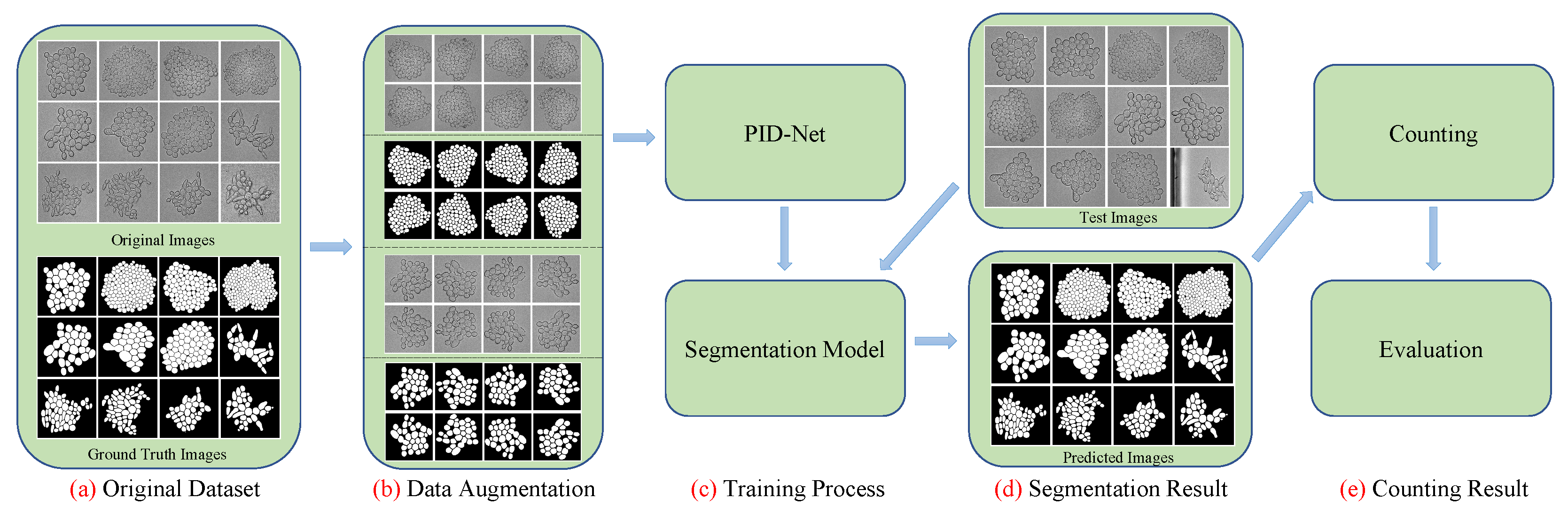
34]-based object counting algorithms, the accuracy of counting is improved. The workflow of the proposed PID-Net counting method is shown in Figure 1.
In Figure 1, (a) Original Dataset: The dataset contains images of yeast cells and their ground truth (GT). The range is from 1 to 256 yeast cells in each image. (b) Data Augmentation: Mirror and rotation operations are applied to augment the original dataset. (c) Training Process: PID-Net is trained for image segmentation and the best model is generated. (d) Segmentation Result: Test images are processed using the trained PID-Net model and output the predicted segmentation results. (e) Counting Result: The number of yeast cells is counted by using connected domain detection.
The main contributions of this paper are as follows:
  • We propose PID-Net for dense tiny object counting. MaxPooling and pixel interval down-sampling are concatenated as down-sampling to extract spatial local and global features.
  • The operation of max-pooling may lose some local features of tiny objects while segmentation, and the edge lines may not be connected after max-pooling. However, the PID-Net can cover a more detailed region.
  • The proposed PID-Net achieves better counting performance than other models on the EM (yeast) counting task.
The paper is organized as follows: Section 2 is the related work of existing image analysis-based microorganism counting methods. Section 3 describes the architecture of the proposed PID-Net in detail. Section 4 consists of the experimental setting, evaluation metrics and results. Section 5 is the conclusion of this paper.

2. Related Work

In this section, related approaches to image analysis-based microorganism counting methods are summarized in Table 1, which consist of classical counting methods and machine-learning-based counting methods. More detailed research can be referred to in our survey paper [28].

2.1. Classical Counting Methods

Image segmentation is the most significant part in microorganism-counting task. As shown in Table 1, the classical methods contain thresholding, edge detection and watershed methods [56]. For thresholding approaches, the selection of threshold determines the result of segmentation. The most used approaches are iterative thresholding and Otsu thresholding at present. Otsu thresholding can achieve satisfactory segmentation results for most images [57].
Edge detection approaches can extract all boundaries in an image, and then each close region can be separated [58]. Watershed is one kind of region-based segmentation approach, which can be calculated by iterative labeling [59]. The satisfactory segmentation result can be received though in an image with weak edges. Hough transformation was proposed for line or circle detection tasks in image with strong anti-noise capability and high accuracy, which can be applied for circular microorgansim counting tasks [60].
In [35,36,37], various thresholding methods were applied for microorganism counting. In [35], an adaptive thresholding was used for microorganism segmentation, and after that, the minima function was applied to locate the center of each colony for counting. The work [36] applied Otsu thresholding for bacteria segmentation, and the hypothesis testing was then applied for debris erasing. In [37], the contrast-limited adaptive histogram equalization was applied to enhance the plate contour first. Then, the Otsu threshold was applied to detect the plate region and binarize the images automatically. Finally, the colonies were separated and counted.
The works [38,39,40] used several edge detection methods for microorganism counting. In [38], five different combination methods applying for microorganism segmentation were compared, such as Gaussian Laplacian and Canny filters. Then, the concave surface between the connected colonies was detected for counting. The works [39,40] used Sobel and Laplacian filters for the edge detection of bacteria images.
The works [41,42,43,44] use watershed-based methods for microorganism counting. In [41], watershed was applied for separation of clustered colonies of bacteria images. After that, the circularity ratio was calculated for colony counting. In [42], marker-controlled watershed was applied for bacteria segmentation. Then, the number of colonies was estimated as the ratio of cluster area to an average colony area. In [43], Otsu and adaptive thresholding were applied for image binarization. Then, the combination method of distance transform and watershed was applied for bacteria counting. In [44], watershed was used for image segmentation. After that, the gray level co-occurrence matrix (GLCM) of the image was extracted and classified using SVM.
The works [45,46,47] used Hough-transformation-based methods for microorganism counting. In [45], the iterative local threshold was used for bacteria segmentation, and then a Hough circle transformation was applied to separate clustered colonies into a single colony. In [46], a median filter was applied for denoising. Then, the circular area was detected using the Hough transform to obtain only the inner area of the dish. Afterward, Gaussian adaptive thresholding was applied for bacteria segmentation. Finally, cross correlation-based granulometry was used to count the bacteria colonies. In [47], Otsu thresholding and a Laplacian filter were applied for edge detection. Then, a circular Hough transform was used to detect circular bacteria colonies.

2.2. Machine-Learning-Based Counting Methods

As shown in Table 1, the machine-learning-based microorganism counting approaches consist of machine-learning- and deep-learning-based methods. The classical machine-learning-based approaches contain Principal Component Analysis (PCA) [61] and Support Vector Machine (SVM) [62]. Deep-learning methods are usually based on CNN [63], Back Propagation Neural Network (BPNN) [64] and Artificial Neural Network (ANN) [65] algorithms.
The works [48,49,50,51] used classical machine learning for microorganism counting. In [48], PCA was applied for separation the bacteria with other debris. After that, the nearest neighbor searching algorithm was applied for clustered colony separation. In [49], the shape features were extracted for training, then the SVM was applied for microorganism classification and counting after Otsu thresholding.
In [50], the histogram local equalization was applied to enhance the contours of protozoa images. Then, morphological erosion and reconstruction were used to eliminate the flocs of the protozoa silhouette. Finally, PCA was applied to classify different protozoa, and the number of the various species of protozoa was counted. In [51], local auto-correlational masks were used for image enhancement, and PCA was applied for plankton counting.
The works [52,53,54,55] used deep learning for microorganism classification and counting. In [52], the Marr–Hildreth operator and thresholding were applied for edge detection and binarization of bacteria images. Then, ANN was designed for classification and counting. In [53], the contrast-limited adaptive histogram equalization was applied for bacteria image segmentation, then four convolutional and one fully connected was trained for classification and counting. In [54], contrast limited adaptive histogram equalization was used for image enhancement.
Then, CNN was applied for bacteria classification, and the watershed algorithm was applied for colony separation and counting. In [55], a classification-type convolutional neural network (cCNN) was proposed for automatic bacteria classification and counting. First, the original images were segmented with an adaptive binary thresholding method, and images with individual cells or cell clusters were cropped. Then, the images were classified using cCNN. The network can output the number of bacteria in given clusters, and the total count can be calculated.
By reviewing all related works of microorganism counting, we found that deep learning technologies are widely applied for microorganism classification; however, few machine-learning-based image segmentation methods are applied. Since the development of deep learning and computer vision technologies, CNN-based image segmentation approaches have be applied for accurate microorganism segmentation, such as SegNet [33], U-Net [34], Attention U-Net [66], Trans U-Net [67] and Swin U-Net [68]. Though the methods above have not been applied for microorganism-counting tasks, they have enough potential to extract the microorganism before counting, which can be inferred with better performance.
Since the yeast images in our dataset range from 1 to 256 yeast cells in each image, and the boundaries of the cells are not clear, it can be inferred that the classical segmentation methods may show poor performance in this counting task. Therefore, we propose an encoder–decoder model that concentrates on the dense and tiny object counting task.

3. PID-Net-Based Yeast Counting Method

Although the existing image segmentation models, such as SegNet and U-Net, have been widely applied in semantic segmentation and biomedical image segmentation, they still cannot meet the requirements of accurate segmentation in the microorganism-counting task. To this end, we propose PID-Net, a CNN-based on pixel interval down-sampling, MaxPooling and concatenate operations to obtain a better performance. The process of microorganism counting mainly contains two parts, the first is microorganism image segmentation, whose purpose is to classify the foreground and background at the pixel-level. The second part is microorganism counting, whose purpose is to count the number of segmented objects after post-processing.

3.1. Basic Knowledge of SegNet

SegNet is a CNN-based image segmentation network with the structure of an encoder and decoder. The innovation of SegNet is that the dense feature maps of high resolution images can be calculated by the encoder, and the up-sampling operation for low-resolution feature maps can be performed by the decoder network [33]. The structure of SegNet can be considered as an encoder network and a corresponding decoder network. The last part is a pixel-level classification layer.
The first 13 convolutional layers of VGG16 [69] is applied in encoder network of SegNet, which consist of convolutional layers, pooling layers and Batch Normalization layers. In the encoder network, two sequences, which consist of one 3 × 3 convolution operation, followed by a Batch Normalization and a ReLU operation, are applied in each step. After that, the feature maps are down-sampled by using a max-pooling operation with the size of 2 × 2 and stride of 2 pixels. After pooling, the size of the feature map is changed into half of the initial.
What is noteworthy is that the Pooling Indices are saved while pooling, which records the initial position of the maximum value in the input feature maps. In the decoder network, the up-sampling operation is applied for feature maps, and then the convolution operation is performed three times to fix the detail loss while pooling. The same operation is replicated five times to change the feature maps into the initial image size. The saved Pooling Indices are applied while up-sampling to set the feature points into correct positions. A Softmax layer is applied finally for feature map classification.

3.2. Basic Knowledge of U-Net

U-Net is an U-shape CNN model based on an encoder–decoder and skip connection. U-Net is first designed for the segmentation of biomedical images. The max-pooling with the size of 2 × 2 and stride of 2 pixels is applied for down-sampling. There are two 3 × 3 convolution operations (each followed by a ReLU) between two down-sampling operations. The down-sampling operation repeats four times, and the number of feature map channels is modified to 1024.
In the decoder network, the result after up-convolution operation (a 2 × 2 up-sampling and a 2 × 2 convolution operation) is concatenated with the corresponding feature maps of encoder, which can combine the high-level semantics with the low-level fine-grained information of the image. After that, two 3 × 3 convolution operations (each followed by a ReLU) are applied. The size of each feature map is changed into the size of input after four up-sampling operations. Finally, a Sigmoid function is applied for classification.

3.3. The Structure of PID-Net

Following the basic idea of SegNet and U-Net for image segmentation, the structure of the proposed PID-Net is shown in Figure 2, which is an end-to-end CNN structure based on the encoder and decoder. There are four blocks in the encoder network.
The first parts in each block are two convolution operations with a kernel size of 3 × 3 (each followed by a ReLU operation), and then the max-pooling with the size of 2 × 2 and stride of 2 pixels is applied to reduce the size of feature maps by half, followed by a convolution and ReLU operation. The channel of feature maps is denoted as C. Pixel interval down-sampling is applied for down-sampling, which is shown in Figure 2. Each pixel is sampled with the pixels apart, and the size of each feature map is replaced by half.
The classical down-sampling methods, such as max-pooling (with the kernel size of 2) will drop 3 4 data of the original image. It can retain the main information but not be fit to the task of tiny object counting (the edge lines may be lost while max-pooling). Though there are several learnable pooling layers that have proposed, such as Fractional pooling [70], Stochastic pooling [71] and learned-norm pooling approaches [72]; however, they still cannot meet the requirement of accurate segmentation for dense tiny yeast cells.
Thus, a new down-sampling method, pixel interval down-sampling, is proposed here, which can reduce the size of feature maps without dropping data. Afterward, four pixel interval down-sampling feature maps and the features after max-pooling are concatenated to 5C-dimensional features. Finally, a convolutional filter with C channels is applied to reduce 5C-dimensional features to C-dimensional features. Hereto, the initial feature maps with size H × W and channel C are changed to feature maps with size H 2 × W 2 and channel C. The procedure is repeated four times with output resolutions of H 16 × W 16 and channel of 8C.
In the decoder network, four blocks are applied for up-sampling. Two convolution operations with a kernel size of 3 × 3 (each followed by a ReLU operation) are applied first. Then, the transposed convolution operation with a kernel size of 3, a stride of 2 and padding of 1 is applied for up-sampling. The transposed convolution operation is widely applied in GANs to expand the size of images [73]. The count of channels after up-sampling of the bottleneck is 512, which is calculated by using the transposed convolutional filter with 512 channels [74].
The params in the transposed convolution filter can be learned while training. After that, the high resolution feature maps of encoder network are transformed to low-resolution feature maps using 2×, 4× and 8× max-pooling, which is shown in Figure 2. Then, the feature maps after up-sampling and max-pooling are concatenated with the feature maps generated by the corresponding layer from the encoder.
For instance, the 8× max-pooling features of the first block, 4× max-pooling of the second block and 2× max-pooling of the third block in the encoder are concatenated with the copied features of the fourth encoder block and the features after up-sampling (five parts of feature maps are concatenated in the first decoder block). In the same way, there are 4, 3 and 2 parts of features are concatenated in the second, third and fourth level of the decoder, respectively. After the concatenated operation, two convolutions and ReLU operations are applied to change the number of channels. The up-sampling operation is repeated four times with output resolutions of H × W and channel of C, which has the same size as the encoder’s input features. Finally, a Softmax layer with two output channels is applied for feature map classification.

3.4. Counting Approach

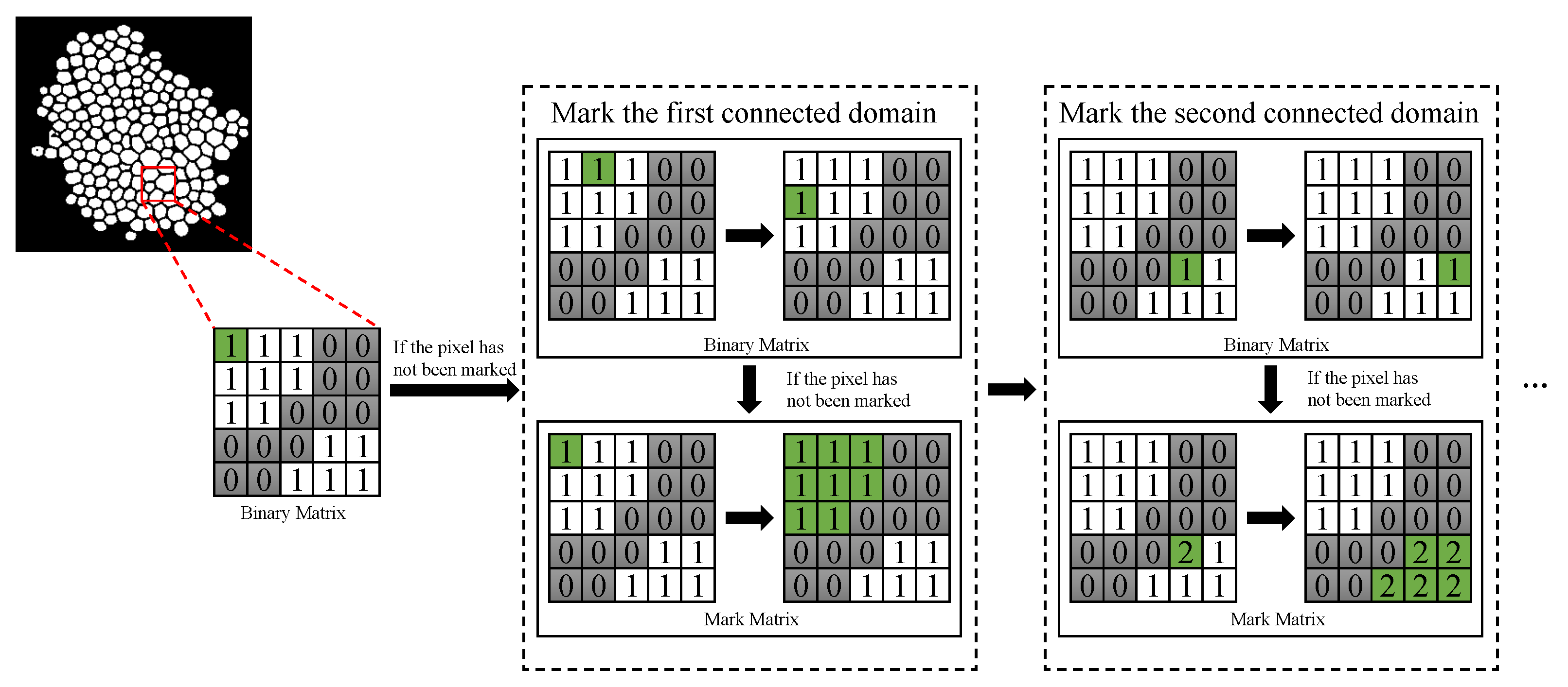
A post-processing method is applied to eliminate the effect of noises after segmentation. First, a morphological filter is applied to remove useless debris, which can improve the performance of counting prominently. Then, the eight neighborhood search algorithm is applied to count the connected regions of segmented images after denoising [75]. The process of counting is shown in Figure 3. A binary matrix is traversed in line and a mark matrix is applied to mark the connected domain [76]. Finally, the number of connected domain in mark matrix is the number of yeast cells.

4. Experiments

4.1. Experimental Setting

4.1.1. Image Dataset

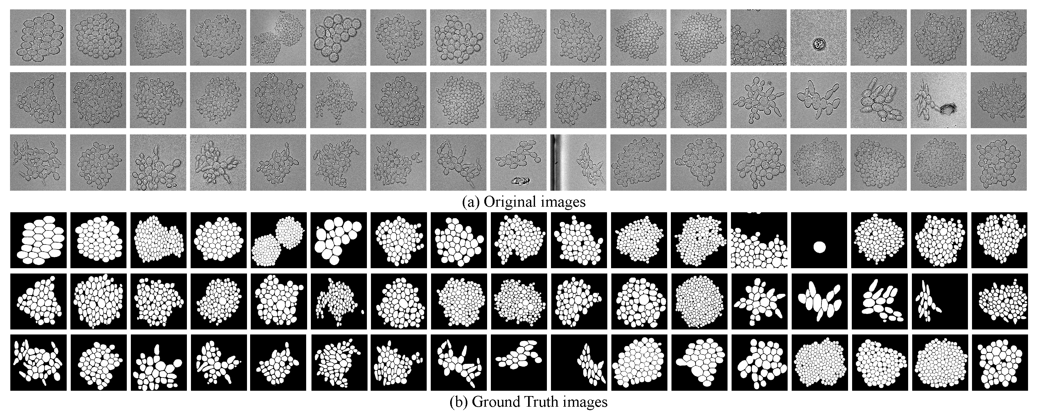
In our work, we use a yeast image dataset proposed in [77], containing 306 different images of yeast cells and their corresponding ground truth (GT) images. All images are resized to the resolution of 256 × 256 pixels, which are shown in Figure 4. Then, the original 306 images are rotated (0, 90, 180 and 270 degrees) and flipped (mirror), and thus the number of images in this dataset is augmented to eight times (2448 images).

4.1.2. Training, Validation and Test Data Setting

The original yeast image dataset was randomly divided into training, validation and test dataset with the ratio of 3:1:1, and then, each dataset was augmented eight times. Therefore, there 1470 images with their GT were applied as the training dataset, 489 images with their corresponding GT were applied for validation, and 489 original images were applied for testing.

4.1.3. Experimental Environment

The experiment was conducted by Python 3.8.10 in Windows 10 operating system. The experimental environment was based on Torch 1.9.0. The workstation was equipped with Intel(R) Core(TM) i7-8700 CPU with 3.20 GHz, 16 GB RAM and NVIDIA GEFORCE RTX 2080 8 GB.

4.1.4. Hyper Parameters

In the experiment of yeast cell counting, the purpose of image segmentation is to determine whether a pixel is a foreground (yeast cell) or background. The last part in the proposed PID-Net before the output is Softmax, which is applied to calculate the classification result of feature maps. The definition of Softmax is shown as Equation (1).
Softmax ( z i ) = e z i c = 1 C e z c .
In Equation (1), z i is the output in the ith node, and C is the number of output nodes, representing the number of classified categories. The classification prediction can be converted into the probabilities by using the Softmax function, which distributes in the range of [0, 1], and the sum of probability is 1. As the image segmentation for yeast counting is to distinguish the foreground and the background. Hence, it is a binary classification, Equation (1) can be rewritten as Equation (2).
Softmax ( z 1 ) = e z 1 e z 1 + e z 2 = 1 1 + e ( z 1 z 2 ) = Sigmoid ( β ) .
In Equation (2), β is ( z 1 z 2 ) , which means the Softmax function and the Sigmoid function are the same for binary classification (a little difference between them is, the number of the fully connected (FC) layer of Softmax is two to distinguish two different categories; however, the number of FC layer of Sigmoid is one, only to judge whether the single pixel is the object to be segmented).
The probability of the pixel to be classified as 1 is:
y ^ = P ( y = 1 | x ) .
Apparently, the probability of the pixel to be classified as 0 is:
1 y ^ = P ( y = 0 | x ) .
According to the maximum likelihood formula, the joint probability can be expressed as:
P ( y | x ) = y ^ y · ( 1 y ^ ) 1 y .
After that, l o g function is applied to remain the monotonicity invariance of the function:
l o g P ( y | x ) = l o g ( y ^ y · ( 1 y ^ ) 1 y ) = y l o g y ^ + ( 1 y ) l o g ( 1 y ^ ) .
Hereto, the loss can be expressed as l o g P ( y | x ) , and the loss function for multiple samples can be defined as the cross-entropy loss (N is the number of categories):
L o s s = [ i = 1 N y ( i ) l o g y ^ ( i ) + ( 1 y ( i ) ) l o g ( 1 y ^ ( i ) ) ] .
In order to guarantee the stable and fast convergence of the proposed network, we deploy preliminary experiments to determine the choices of hyper parameters. Adaptive moment estimation (Adam) is compared with stochastic gradient descent (SGD) and natural gradient descent (NGD). Adam optimizer has the smoothest loss curves and stablest convergence, which performs best in microorganism-counting task. Adam optimizer is applied to minimize the loss function, which can adjust the learning rate automatically by considering the gradient momentum of the previous time steps [78].
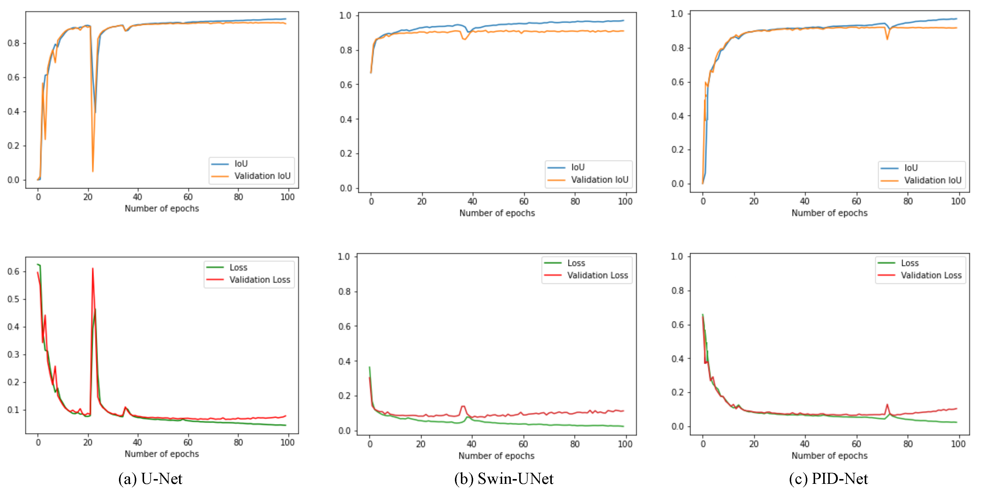
The initial learning rate is set from 0.0001 to 0.01 in preliminary experiments. By observing the loss curves while training, the learning rate of 0.001 can balance the speed and stability of convergence. The batch size is set as 8 due to the limited memory size (8 GB). The selection of the hyper parameters above are optimal in preliminary experiments, and thus they are applied in our formal microorganism counting experiment. The epoch is set as 100 by considering the converge speed of experimental models, the example of loss and intersection over union (IoU) curves of models is shown in Figure 5.
Though there are 92,319,298 params to be trained in PID-Net; however, it can converge rapidly and smoothly without over fitting. There is a jump in loss and IoU plots for all three tested networks from 20 to 80 epochs, which is caused by the small batch size. Small batch size may lead to huge difference between each batch, and the loss and IoU curves may jump with convergence.

4.2. Evaluation Metrics

In the task of dense tiny object counting, the evaluation of image segmentation is the most significant part. Hence, the widely applied segmentation evaluation metrics Accuracy, Dice, Jaccard and Precision are employed here to evaluate the performance of microorganism segmentation. Furthermore, the Hausdorff distance is applied to evaluate the shape similarity between the predicted image and GT. Finally, the counting accuracy is calculated to quantify the counting performance of the models.
Accuracy is applied to calculate the proportion of pixels that are correctly classified. The Dice coefficient [79] is applied to measure the similarity of the predicted image and GT. The similarity can be quantified range from 0 to 1 (1 means the predicted result coincides exactly with the GT). Jaccard [80], also named the intersection over union (IoU), is applied to compare the similarity and differences between the predicted image and GT image, focusing on whether the samples’ common characteristics are consistent. Precision is defined as the proportion of positive pixels in the pixels, which are classified as positive.
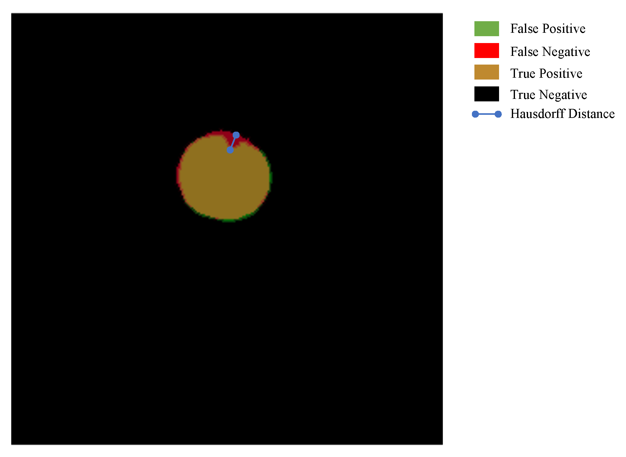
The Hausdorff distance [81] is applied to measure the Euclidean distance between the predicted and GT images with the unit of pixels in per image. In contrast with Dice, the Hausdorff distance focuses on the boundary distance of two objects to measure the shape similarity; however, the Dice majors in the inner similarity. An example of the Hausdorff distance between GT and predicted image is shown in Figure 6. The Hausdorff is the maximum of the shortest distance between a pixel in a image and another image [82].
In the task of microorganism counting, the Hausdorff distance can be applied to measure the shape similarity between the GT and segmentation result, showing the performance of segmentation models. Finally, the performance of counting is measured using counting accuracy, which is defined as the proportion of the predicted number and GT number of yeast cell images.
The definitions of the proposed evaluation metrics are summarized in Table 2. The TP (True Positive), TN (True Negative), FP (False Positive) and FN (False Negative) are basic evaluation metrics, which can be applied to measure the performance of segmentation in general. An example of a yeast cell image with its TP, TN, FP and FN is illustrated in Figure 7 for intuitive understanding. V p r e d is the foreground after segmentation by using the model, V G T is the foreground of the GT image. Furthermore, N p r e d means the number of connected regions in the predicted image, N G T means the number of connected regions in the GT image, which indicates the number of yeast cells. In the definition of the Hausdorff distance, s u p is the supremum, and i n f is the infimum.
The proposed evaluation metrics, containing the Accuracy, Dice, Jaccard and Precision, are proportional to the segmentation performance of models. The Hausdorff distance has an inverse correlation with the segmentation performance. Counting accuracy can evaluate the final counting results of different models.

4.3. Evaluation of Segmentation and Counting Performance

To prove the satisfactory segmentation performance of the proposed PID-Net for dense tiny object counting, we compare different down-sampling methods to show the advancement of our proposed method. Furthermore, several state-of-the-art approaches are applied for comparative experiments. All of the experimental setting and evaluation indices are same for comparative experiment. Furthermore, the same dataset is applied for all comparative experiments, which is proposed in Section 4.1.1. The models are trained from scratch without pre-training and fine-tuning.

4.3.1. Comparison of Different Down-Sampling Methods

In this part, we compare the effect of different down-sampling and skip connection approaches for segmentation. In our proposed PID-Net, pixel interval down-sampling and max-pooling operations are concatenated to combine the dense and sparse feature maps after convolution operations. Then, in the process of hierarchy skip connection, max-pooling is applied to combine the high-level features and low-level features directly, which is beneficial to reduce the effect of resolution loss while up-sampling and help rebuild the segmentation result.
To show the effectiveness and reasonability of the proposed method, we change the approaches of down-sampling and hierarchy skip connection as PID-Net Modified-1 (PID-Net-M1) and PID-Net Modified-2 (PID-Net-M2). In PID-Net-M1, max-pooling operations are only applied in the process of hierarchy skip connection and not in down-sampling. The down-sampling block of PID-Net-M1 is illustrated in Figure 8. In PID-Net-M2, all down-sampling operations are realized using pixel interval down-sampling without max-pooling. The segmentation evaluations and counting performance of those approaches are shown in Table 3.
From Table 3, we find that the proposed PID-Net achieves the best counting performance. By comparing with the PID-Net-M1 and PID-Net-M2, the average accuracy is increased by 0.1% to 0.6%; the improvement of average Dice value is 0.1% to 1.1%; the average Jaccard is improved by around 0.3% to 1.6%. Furthermore, the mean Hausdorff distance of PID-Net is the shortest, which indicates the similarity between the predicted images and GT images is the highest. Finally, the counting accuracy achieved 96.97%, which shows the satisfactory counting performance of the PID-Net. Hence, the segmentation and counting performance of PID-Net is the best by referring to all evaluation metrics.

4.3.2. Comparison with Other Methods

In this part, some comparative experiments are applied for the yeast cell counting task. Some classical methods proposed in Section 2 and deep-learning-based methods proposed in Section 3 are compared, consisting Hough transformation [83], Otsu thresholding, Watershed, SegNet and U-Net-based segmentation approaches. Furthermore, we conduct some extra experiments using state-of-the-art approaches, containing Attention U-Net [66], Trans U-Net [67] and Swin U-Net [68].
Due to the determination of k in clustering methods, such as k-means, is still an insoluble problem while counting; therefore, the clustering-based approaches cannot be applied here for dense tiny object counting. All comparative experiments have the same experimental setting, which can be referred to Section 4.1 for details. After image segmentation and object counting, the average evaluation indices are summarized in 
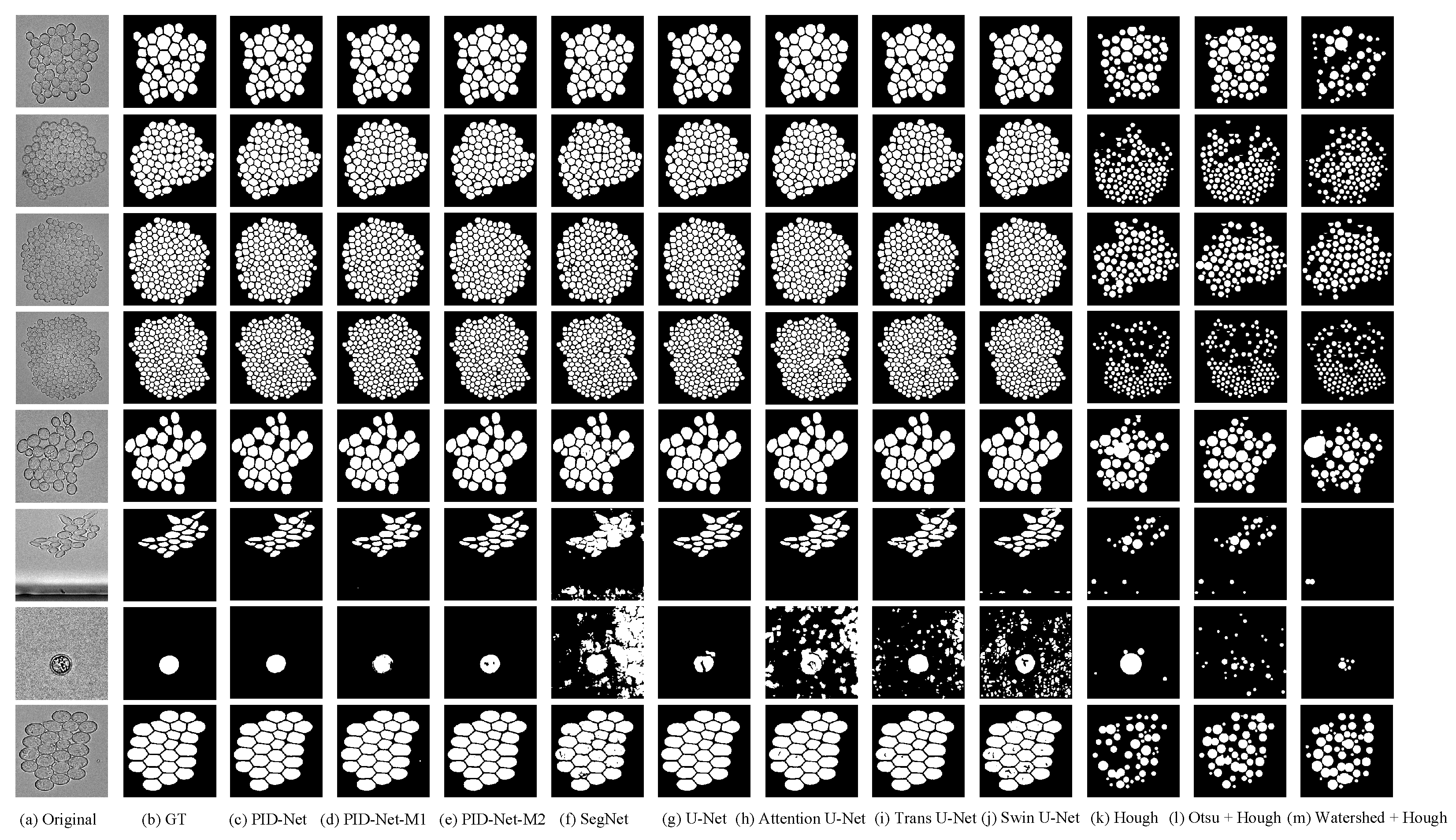
Table 4, and the example images of segmentation are shown in Figure 9.
From the evaluation indices summarized in Table 4, we can find that the PID-Net has the highest Accuracy, Dice, Jaccard, Precision and Counting Accuracy and the lowest Hausdorff distance, which means the proposed model performs best in the task of dense tiny object counting by comparing with other models. Even more, the Jaccard of PID-Net is higher than the YeaZ who proposed this yeast cell dataset. In general, the approaches based on deep learning perform better than the classical approaches.
We find that the Counting Accuracy of several methods are very low abnormally, which may caused by the enormous difference between the GT and the predicted image. For instance, the single yeast cell image in Figure 9 performs unsatisfactory when the segmentation is not accurate. The segmentation results of SegNet and Attention-UNet have a large number of False Positive pixels, and the counting approach is based on the connected domain detection; hence, the value of | N p r e d N G T | N G T is much higher than normal.
From the best performance of the proposed PID-Net in the task of dense tiny object counting, we can infer that the down-sampling and skip connection part of PID-Net, which combines max-pooling and pixel interval down-sampling can obtain the feature maps of dense tiny objects and reconstruct the images better.

4.4. Repeatability Tests

Five additional experiments were repeated based on the original PID-Net model for repeatability tests. The evaluation indices are given in Table 5. From Table 5, we find that all evaluation indices of repeated PID-Nets are approximate, which shows satisfactory and stable counting performance for the dense tiny object counting task.

4.5. Computational Time

The training time, mean training time, test time and mean test time are listed in Table 6. There are 1470 images in the training dataset and 489 images in the test dataset. The mean training time of PID-Net model is approximately 2.9 s higher than the time of U-Net, and the test time is about 0.4 s higher than U-Net. The memory cost of PID-Net is about 20MB, which is about 6 MB more than the cost of U-Net model, meanwhile, the PID-Net has better counting performance and lower memory cost than Swin-UNet (41 MB). The counting accuracy is increased about 6%; hence, the PID-Net has satisfactory counting performance and a tolerable computational time, which can be widely applied in accurate dense tiny object counting tasks.

4.6. Discussion

Deep learning is essentially to build a probability distribution model driven by data. Therefore, as the deep-learning-network architecture becomes deeper, the quantity and quality of training data will have a greater impact on the performance of the model. However, in the imaging process of microorganism images, the amount of satisfactory data is relatively small due to some objective reasons, such as the impurities in the acquisition environment, uneven natural light and other adverse factors, which leads to insufficient training and poor performance in various tasks. Though the proposed PID-Net has excellent segmentation and counting performance for images with dense tiny objects, there still exists some mis-segmentation, causing the decrease of counting accuracy. Several incorrect segmentation results are shown in Figure 10.
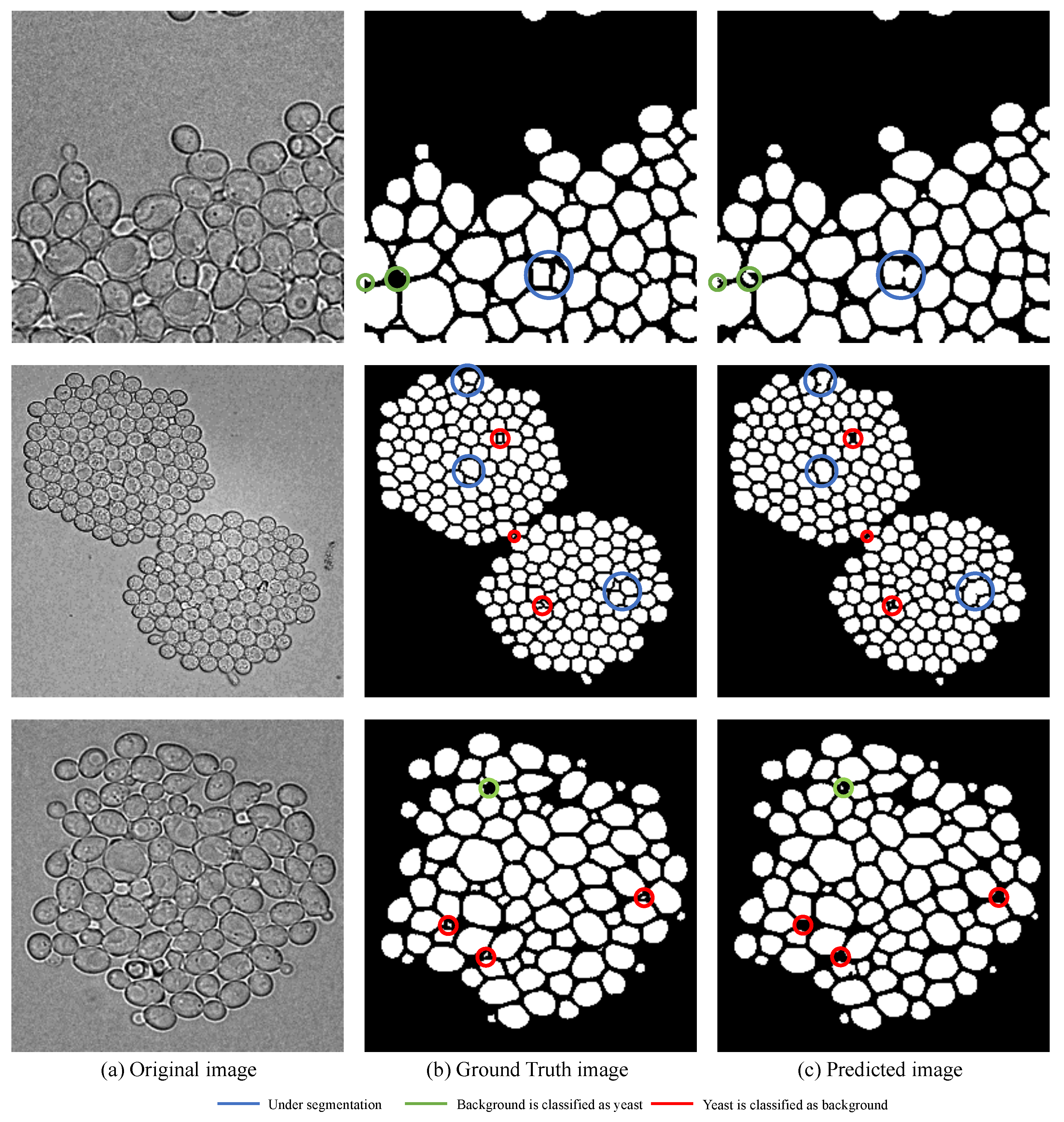
There are three main problems for segmentation and counting, which are illustrated in Figure 10. The blue circle refers to the situation of under segmentation—that is, the neighbor yeast cells cannot be segmented, and the edges cannot be detected. Due to the counting method is based on the eight neighborhood search algorithm, the situation leads to under estimation of the real count of yeast cells. The green circle refers to a part of background is classified as yeast cells. As shown in Figure 10, most of the images are full of dense tiny yeast cells with irregular shapes, and the limitation of small dataset leads to inadequate training.
Therefore, the background between yeast cells with irregular shape is easily classified as a yeast cell, which results in over estimation of the real count of yeast cells. On the contrary, the red circle represents the part of yeast cell is classified as background. There are 1 to 256 yeast cells with different sizes in a single image in this dataset, and thus the shape and size of yeast cells have a great difference. Therefore, the tiny yeast cell between the larger cells has a great similarity with the background, which is difficult for models to discriminate especially in a small dataset. The situation leads to under estimation of the real count of yeast cells.
The situations of adherent yeast cells and mis-segmentation lead to counting error. Moreover, the training data is limited due to the small dataset; therefore, the models cannot be trained perfectly. The small dataset is a limitation of the yeast counting task. However, despite some cases of mis-segmentation, most of the yeast cells in the test dataset could be detected and segmented with other cells. The segmented region might be small but has little effect on the counting results calculated using the eight neighborhood search algorithm.

5. Conclusions and Future Work

In this paper, a CNN-based PID-Net was proposed for dense tiny objects (yeast) counting task. The PID-Net is an end-to-end model based on an encoder–decoder structure, and we proposed a new down-sampling model consisting of pixel interval down-sampling and max-pooling, which can serve to extract the dense and sparse features in the task of dense tiny object counting. By comparing with the proposed PID-Net and classical U-Net-based yeast counting results, the evaluation indices of Accuracy, Dice, Jaccard, Precision, Counting Accuracy and Hausdorff Distance of PID-Net were 97.51%, 95.86%, 92.10%, 96.02%, 96.97% and 4.6272, which are improved by 0.04%, 0.15%, 0.26%, 0.4% and 5.7%, respectively, and the Hausdorff Distance decreased by 0.0394.
Although the small image dataset resulted in some cases of mis-segmentation, the proposed PID-Net showed a more satisfactory segmentation performance than the other models in the task of dense tiny object counting on a small dataset.
In the future, we plan to apply PID-Net for more dense tiny object counting tasks, such as the streptococcus counting task and blood-cell-counting task. We will further optimize the PID-Net for better counting performance. For instance, object separation is one of the most significant parts in object counting; therefore, the Contour Loss [84] can be used by referring to our work to distinguish inner texture and contour boundaries for more accurate counting. We also consider using Knowledge Distillation [85] to reduce the memory cost of PID-Net, which can help to deploy the model on portable equipment.

Author Contributions

J.Z. (Jiawei Zhang): methodology, software, validation, formal analysis, data curation, writing—original draft preparation, review and editing and visualization; X.Z.: resources; T.J.: investigation and funding acquisition; M.M.R.: validation; Y.Y.: validation; Y.-H.L.: validation; J.Z. (Jinghua Zhang): formal analysis; A.P.: investigation; M.G.: investigation and C.L.: conceptualization, methodology, data curation, writing—original draft preparation, writing—review and editing, supervision and project administration. All authors have read and agreed to the published version of the manuscript.

Funding

This work was funded by the “National Natural Science Foundation of China” (No. 61806047) and the “Sichuan Science and Technology Plan” (No. 2021YFH0069, 2021YFQ0057, 2022YFS0565).

Data Availability Statement

Yeast dataset can be found at: https://www.epfl.ch/labs/lpbs/data-and-software/ (accessed on 16 January 2021).

Acknowledgments

We thank Zixian Li and Guoxian Li for their important discussion.

Conflicts of Interest

There is no conflict of interest in this paper.

Abbreviations

The following abbreviations are used in this manuscript:
PID-Netpixel interval down-sampling network
CNNconvolutional neural network
EMsenvironmental microorganisms
SVMsupport vector machine
PCAprincipal-component analysis
BPNNback propagation neural network
ANNartificial neural network
ReLUrectified linear unit
Adamadaptive moment estimation
SGDstochastic gradient descent
NGDnatural gradient descent
GTground truth
FCfully connected
IoUintersection over union
TPtrue positive
TNtrue negative
FPfalse positive
FNfalse negative

References

  1. Yu, M.; Wang, J.; Tang, L.; Feng, C.; Liu, H.; Zhang, H.; Peng, B.; Chen, Z.; Xie, Q. Intimate coupling of photocatalysis and biodegradation for wastewater treatment: Mechanisms, recent advances and environmental applications. Water Res. 2020, 175, 115673. [Google Scholar] [CrossRef]
  2. Wang, Y.; Qiu, L.; Hu, M. Application of yeast in the wastewater treatment. EDP Sci. 2018, 53, 04025. [Google Scholar] [CrossRef]
  3. You, L.; Zhao, D.; Zhou, R.; Tan, Y.; Wang, T.; Zheng, J. Distribution and Function of Dominant Yeast Species in the Fermentation of Strong-flavor Baijiu. World J. Microbiol. Biotechnol. 2021, 37, 26. [Google Scholar] [CrossRef]
  4. Balestra, G.; Misaghi, I. Increasing the Efficiency of the Plate Counting Method for Estimating Bacterial Diversity. J. Microbiol. Methods 1997, 30, 111–117. [Google Scholar] [CrossRef]
  5. Sambrook, J.; Russell, D.W. Estimation of Cell Number by Hemocytometry Counting. Cold Spring Harb. Protoc. 2006, 2006, pdb–prot4454. [Google Scholar] [CrossRef]
  6. Gasol, J.M.; Del Giorgio, P.A. Using Flow Cytometry for Counting Natural Planktonic Bacteria and Understanding the Structure of Planktonic Bacterial Communities. Sci. Mar. 2000, 64, 197–224. [Google Scholar] [CrossRef] [Green Version]
  7. Li, X.; Li, C.; Rahaman, M.M.; Sun, H.; Li, X.; Wu, J.; Yao, Y.; Grzegorzek, M. A comprehensive review of computer-aided whole-slide image analysis: From datasets to feature extraction, segmentation, classification and detection approaches. Artif. Intell. Rev. 2022, 55, 4809–4878. [Google Scholar] [CrossRef]
  8. Li, Y.; Li, C.; Li, X.; Wang, K.; Rahaman, M.M.; Sun, C.; Chen, H.; Wu, X.; Zhang, H.; Wang, Q. A Comprehensive Review of Markov Random Field and Conditional Random Field Approaches in Pathology Image Analysis. Arch. Comput. Methods Eng. 2021, 29, 609–639. [Google Scholar] [CrossRef]
  9. Zhou, X.; Li, C.; Rahaman, M.M.; Yao, Y.; Ai, S.; Sun, C.; Wang, Q.; Zhang, Y.; Li, M.; Li, X.; et al. A comprehensive review for breast histopathology image analysis using classical and deep neural networks. IEEE Access 2020, 8, 90931–90956. [Google Scholar] [CrossRef]
  10. Li, C.; Chen, H.; Li, X.; Xu, N.; Hu, Z.; Xue, D.; Qi, S.; Ma, H.; Zhang, L.; Sun, H. A review for cervical histopathology image analysis using machine vision approaches. Artif. Intell. Rev. 2020, 53, 4821–4862. [Google Scholar] [CrossRef]
  11. Liu, W.; Li, C.; Rahaman, M.M.; Jiang, T.; Sun, H.; Wu, X.; Hu, W.; Chen, H.; Sun, C.; Yao, Y.; et al. Is the aspect ratio of cells important in deep learning? A robust comparison of deep learning methods for multi-scale cytopathology cell image classification: From convolutional neural networks to visual transformers. Comput. Biol. Med. 2022, 141, 105026. [Google Scholar] [CrossRef]
  12. Rahaman, M.M.; Li, C.; Yao, Y.; Kulwa, F.; Wu, X.; Li, X.; Wang, Q. DeepCervix: A deep learning-based framework for the classification of cervical cells using hybrid deep feature fusion techniques. Comput. Biol. Med. 2021, 136, 104649. [Google Scholar] [CrossRef]
  13. Rahaman, M.M.; Li, C.; Wu, X.; Yao, Y.; Hu, Z.; Jiang, T.; Li, X.; Qi, S. A survey for cervical cytopathology image analysis using deep learning. IEEE Access 2020, 8, 61687–61710. [Google Scholar] [CrossRef]
  14. Zou, S.; Li, C.; Sun, H.; Xu, P.; Zhang, J.; Ma, P.; Yao, Y.; Huang, X.; Grzegorzek, M. TOD-CNN: An effective convolutional neural network for tiny object detection in sperm videos. Comput. Biol. Med. 2022, 146, 105543. [Google Scholar] [CrossRef]
  15. Chen, A.; Li, C.; Zou, S.; Rahaman, M.M.; Yao, Y.; Chen, H.; Yang, H.; Zhao, P.; Hu, W.; Liu, W.; et al. SVIA dataset: A new dataset of microscopic videos and images for computer-aided sperm analysis. Biocybern. Biomed. Eng. 2022, 42, 204–216. [Google Scholar] [CrossRef]
  16. Ma, P.; Li, C.; Rahaman, M.M.; Yao, Y.; Zhang, J.; Zou, S.; Zhao, X.; Grzegorzek, M. A state-of-the-art survey of object detection techniques in microorganism image analysis: From classical methods to deep learning approaches. Artif. Intell. Rev. 2022, 1–72. [Google Scholar] [CrossRef]
  17. Zhao, P.; Li, C.; Rahaman, M.; Xu, H.; Yang, H.; Sun, H.; Jiang, T.; Grzegorzek, M. A Comparative Study of Deep Learning Classification Methods on a Small Environmental Microorganism Image Dataset (EMDS-6): From Convolutional Neural Networks to Visual Transformers. Front. Microbiol. 2022, 13, 792166. [Google Scholar] [CrossRef]
  18. Kulwa, F.; Li, C.; Zhang, J.; Shirahama, K.; Kosov, S.; Zhao, X.; Jiang, T.; Grzegorzek, M. A new pairwise deep learning feature for environmental microorganism image analysis. Environ. Sci. Pollut. Res. 2022, 29, 51909–51926. [Google Scholar] [CrossRef]
  19. Kosov, S.; Shirahama, K.; Li, C.; Grzegorzek, M. Environmental microorganism classification using conditional random fields and deep convolutional neural networks. Pattern Recognit. 2018, 77, 248–261. [Google Scholar] [CrossRef]
  20. Li, C.; Shirahama, K.; Grzegorzek, M. Environmental microbiology aided by content-based image analysis. Pattern Anal. Appl. 2016, 19, 531–547. [Google Scholar] [CrossRef]
  21. Li, C.; Shirahama, K.; Grzegorzek, M. Application of content-based image analysis to environmental microorganism classification. Biocybern. Biomed. Eng. 2015, 35, 10–21. [Google Scholar] [CrossRef]
  22. Rahaman, M.M.; Li, C.; Yao, Y.; Kulwa, F.; Rahman, M.A.; Wang, Q.; Qi, S.; Kong, F.; Zhu, X.; Zhao, X. Identification of COVID-19 samples from chest X-Ray images using deep learning: A comparison of transfer learning approaches. J. X-ray Sci. Technol. 2020, 28, 821–839. [Google Scholar] [CrossRef]
  23. Zhang, J.; Li, C.; Yin, Y.; Zhang, J.; Grzegorzek, M. Applications of artificial neural networks in microorganism image analysis: A comprehensive review from conventional multilayer perceptron to popular convolutional neural network and potential visual transformer. Artif. Intell. Rev. 2022, 1–58. [Google Scholar] [CrossRef]
  24. Kulwa, F.; Li, C.; Zhao, X.; Cai, B.; Xu, N.; Qi, S.; Chen, S.; Teng, Y. A state-of-the-art survey for microorganism image segmentation methods and future potential. IEEE Access 2019, 7, 100243–100269. [Google Scholar] [CrossRef]
  25. Zhao, P.; Li, C.; Rahaman, M.M.; Xu, H.; Ma, P.; Yang, H.; Sun, H.; Jiang, T.; Xu, N.; Grzegorzek, M. EMDS-6: Environmental Microorganism Image Dataset Sixth Version for Image Denoising, Segmentation, Feature Extraction, Classification, and Detection Method Evaluation. Front. Microbiol. 2022, 13, 1334. [Google Scholar] [CrossRef] [PubMed]
  26. Li, C.; Zhang, J.; Kulwa, F.; Qi, S.; Qi, Z. A SARS-CoV-2 Microscopic Image Dataset with Ground Truth Images and Visual Features. In Chinese Conference on Pattern Recognition and Computer Vision (PRCV); Springer: Cham, Switzerland, 2020; pp. 244–255. [Google Scholar]
  27. Zhang, J.; Xu, N.; Li, C.; Rahaman, M.M.; Yao, Y.D.; Lin, Y.H.; Zhang, J.; Jiang, T.; Qin, W.; Grzegorzek, M. An application of Pixel Interval Down-sampling (PID) for dense tiny microorganism counting on environmental microorganism images. arXiv 2022, arXiv:2204.01341. [Google Scholar]
  28. Zhang, J.; Li, C.; Rahaman, M.M.; Yao, Y.; Ma, P.; Zhang, J.; Zhao, X.; Jiang, T.; Grzegorzek, M. A Comprehensive Review of Image Analysis Methods for Microorganism Counting: From Classical Image Processing to Deep Learning Approaches. Artif. Intell. Rev. 2022, 55, 2875–2944. [Google Scholar] [CrossRef]
  29. Chunhachart, O.; Suksawat, B. Construction and Validation of Economic Vision System for Bacterial Colony Count. In Proceedings of the 2016 International Computer Science and Engineering Conference (ICSEC), Chiang Mai, Thailand, 14–17 December 2016; pp. 1–5. [Google Scholar] [CrossRef]
  30. Choudhry, P. High-throughput Method for Automated Colony and Cell Counting by Digital Image Analysis Based on Edge Detection. PLoS ONE 2016, 11, e0148469. [Google Scholar] [CrossRef] [Green Version]
  31. Minoi, J.L.; Chiang, T.T.; Lim, T.; Yusoff, Z.; Karim, A.H.A.; Zulharnain, A. Mobile Vision-based Automatic Counting of Bacteria Colonies. In Proceedings of the 2016 International Conference on Information and Communication Technology (ICICTM), Kuala Lumpur, Malaysia, 16–17 May 2016; pp. 41–46. [Google Scholar] [CrossRef]
  32. Li, C.; Wang, K.; Xu, N. A Survey for the Applications of Content-based Microscopic Image Analysis in Microorganism Classification Domains. Artif. Intell. Rev. 2019, 51, 577–646. [Google Scholar] [CrossRef]
  33. Badrinarayanan, V.; Kendall, A.; Cipolla, R. SegNet: A Deep Convolutional Encoder-decoder Architecture for Image Segmentation. IEEE Trans. Pattern Anal. Mach. Intell. 2017, 39, 2481–2495. [Google Scholar] [CrossRef]
  34. Ronneberger, O.; Fischer, P.; Brox, T. U-net: Convolutional Networks for Biomedical Image Segmentation. In International Conference on Medical Image Computing and Computer-assisted Intervention; Springer: Cham, Switzerland, 2015; pp. 234–241. [Google Scholar] [CrossRef] [Green Version]
  35. Clarke, M.L.; Burton, R.L.; Hill, A.N.; Litorja, M.; Nahm, M.H.; Hwang, J. Low-cost, High-throughput, Automated Counting of Bacterial Colonies. Cytom. Part A 2010, 77, 790–797. [Google Scholar] [CrossRef] [PubMed] [Green Version]
  36. Zhang, C.; Chen, W.B.; Liu, W.L.; Chen, C.B. An Automated Bacterial Colony Counting System. In Proceedings of the 2008 IEEE International Conference on Sensor Networks, Ubiquitous, and Trustworthy Computing (SUTC 2008), Taichung, Taiwan, 11–13 June 2008; pp. 233–240. [Google Scholar] [CrossRef]
  37. Zhang, C.; Chen, W.B. An Effective and Robust Method for Automatic Bacterial Colony Enumeration. In Proceedings of the International Conference on Semantic Computing (ICSC 2007), Irvine, CA, USA, 17–19 September 2007; pp. 581–588. [Google Scholar] [CrossRef]
  38. Garcia Arnal Barbedo, J. An Algorithm for Counting Microorganisms in Digital Images. IEEE Lat. Am. Trans. 2013, 11, 1353–1358. [Google Scholar] [CrossRef]
  39. Yamaguchi, N.; Ichijo, T.; Ogawa, M.; Tani, K.; Nasu, M. Multicolor Excitation Direct Counting of Bacteria by Fluorescence Microscopy with the Automated Digital Image Analysis Software BACS II. Bioimages 2004, 12, 1–7. [Google Scholar] [CrossRef]
  40. Ogawa, M.; Tani, K.; Yamaguchi, N.; Nasu, M. Development of Multicolour Digital Image Analysis System to Enumerate Actively Respiring Bacteria in Natural River Water. J. Appl. Microbiol. 2003, 95, 120–128. [Google Scholar] [CrossRef] [Green Version]
  41. Ates, H.; Gerek, O.N. An Image-processing Based Automated Bacteria Colony Counter. In Proceedings of the 2009 24th International Symposium on Computer and Information Sciences, Guzelyurt, Turkey, 14–16 September 2009; pp. 18–23. [Google Scholar] [CrossRef]
  42. Selinummi, J.; Seppälä, J.; Yli-Harja, O.; Puhakka, J.A. Software for Quantification of Labeled Bacteria from Digital Microscope Images by Automated Image Analysis. Biotechniques 2005, 39, 859–863. [Google Scholar] [CrossRef] [PubMed] [Green Version]
  43. Brugger, S.D.; Baumberger, C.; Jost, M.; Jenni, W.; Brugger, U.; Mühlemann, K. Automated Counting of Bacterial Colony forming Units on Agar Plates. PLoS ONE 2012, 7, e33695. [Google Scholar] [CrossRef] [Green Version]
  44. Masschelein, B.; Robles-Kelly, A.; Blanch, C.; Tack, N.; Simpson-Young, B.; Lambrechts, A. Towards a Colony Counting System using Hyperspectral Imaging. Imaging Manip. Anal. Biomol. Cells Tissues X 2012, 8225, 822510. [Google Scholar] [CrossRef]
  45. Austerjost, J.; Marquard, D.; Raddatz, L.; Geier, D.; Becker, T.; Scheper, T.; Lindner, P.; Beutel, S. A Smart Device Application for the Automated Determination of E. coli colonies on Agar Plates. Eng. Life Sci. 2017, 17, 959–966. [Google Scholar] [CrossRef] [Green Version]
  46. Boukouvalas, D.T.; Belan, P.; Leal, C.R.L.; Prates, R.A.; Araújo, S.A.D. Automated colony counter for single plate serial dilution spotting. In Iberoamerican Congress on Pattern Recognition; Springer: Cham, Switzerland, 2018; pp. 410–418. [Google Scholar]
  47. Alves, G.M.; Cruvinel, P.E. Customized computer vision and sensor system for colony recognition and live bacteria counting in agriculture. Sens. Transducers 2016, 201, 65. [Google Scholar]
  48. Yoon, S.C.; Lawrence, K.C.; Park, B. Automatic Counting and Classification of Bacterial Colonies using Hyperspectral Imaging. Food Bioprocess Technol. 2015, 8, 2047–2065. [Google Scholar] [CrossRef]
  49. Zhang, R.; Zhao, S.; Jin, Z.; Yang, N.; Kang, H. Application of SVM in the Food Bacteria Image Recognition and Count. In Proceedings of the 2010 third International Congress on Image and Signal Processing, Yantai, China, 16–18 October 2010; Volume 4, pp. 1819–1823. [Google Scholar] [CrossRef]
  50. Motta, M.d.; Pons, M.N.; Vivier, H.; Amaral, A.; Ferreira, E.; Roche, N.; Mota, M. The Study of Protozoa Population in Wastewater Treatment Plants by Image Analysis. Braz. J. Chem. Eng. 2001, 18, 103–111. [Google Scholar] [CrossRef]
  51. Akiba, T.; Kakui, Y. Development of an in Situ Zooplankton Identification and Counting System Based on Local Auto-correlational Masks. In Proceedings of the Oceans’ 97, MTS/IEEE Conference Proceedings, Halifax, NS, Canada, 6–9 October 1997; Volume 1, pp. 655–659. [Google Scholar] [CrossRef]
  52. Blackburn, N.; Hagström, Å.; Wikner, J.; Cuadros-Hansson, R.; Bjørnsen, P.K. Rapid Determination of Bacterial Abundance, Biovolume, Morphology, and Growth by Neural Network-based Image Analysis. Appl. Environ. Microbiol. 1998, 64, 3246–3255. [Google Scholar] [CrossRef] [PubMed] [Green Version]
  53. Ferrari, A.; Lombardi, S.; Signoroni, A. Bacterial Colony Counting by Convolutional Neural Networks. In Proceedings of the 2015 37th Annual International Conference of the IEEE Engineering in Medicine and Biology Society (EMBC), Milan, Italy, 25–29 August 2015; pp. 7458–7461. [Google Scholar] [CrossRef]
  54. Ferrari, A.; Lombardi, S.; Signoroni, A. Bacterial Colony Counting with Convolutional Neural Networks in Digital Microbiology Imaging. Pattern Recognit. 2017, 61, 629–640. [Google Scholar] [CrossRef]
  55. Tamiev, D.; Furman, P.E.; Reuel, N.F. Automated Classification of Bacterial Cell Sub-populations with Convolutional Neural Networks. PLoS ONE 2020, 15, e0241200. [Google Scholar] [CrossRef] [PubMed]
  56. Perez, A.; Gonzalez, R.C. An Iterative Thresholding Algorithm for Image Segmentation. IEEE Trans. Pattern Anal. Mach. Intell. 1987, PAMI-9, 742–751. [Google Scholar] [CrossRef]
  57. Otsu, N. A threshold selection method from gray-level histograms. IEEE Trans. Syst. Man, Cybern. 1979, 9, 62–66. [Google Scholar] [CrossRef] [Green Version]
  58. Magnier, B.; Abdulrahman, H.; Montesinos, P. A review of supervised edge detection evaluation methods and an objective comparison of filtering gradient computations using hysteresis thresholds. J. Imaging 2018, 4, 74. [Google Scholar] [CrossRef] [Green Version]
  59. Levner, I.; Zhang, H. Classification-Driven Watershed Segmentation. IEEE Trans. Image Process. 2007, 16, 1437–1445. [Google Scholar] [CrossRef]
  60. Yuen, H.; Princen, J.; Illingworth, J.; Kittler, J. Comparative study of Hough transform methods for circle finding. Image Vis. Comput. 1990, 8, 71–77. [Google Scholar] [CrossRef] [Green Version]
  61. Jolliffe, I.T.; Cadima, J. Principal component analysis: A review and recent developments. Philos. Trans. R. Soc. A Math. Phys. Eng. Sci. 2016, 374, 20150202. [Google Scholar] [CrossRef] [PubMed]
  62. Vishwanathan, S.; Narasimha Murty, M. SSVM: A Simple SVM Algorithm. In Proceedings of the 2002 International Joint Conference on Neural Networks, Honolulu, HI, USA, 12–17 May 2002; Volume 3, pp. 2393–2398. [Google Scholar] [CrossRef] [Green Version]
  63. Li, Y.; Hao, Z.; Lei, H. Survey of Convolutional Neural Network. J. Comput. Appl. 2016, 36, 2508–2515. [Google Scholar] [CrossRef]
  64. Dai, H.; MacBeth, C. Effects of learning parameters on learning procedure and performance of a BPNN. Neural Netw. 1997, 10, 1505–1521. [Google Scholar] [CrossRef] [Green Version]
  65. Ghate, V.N.; Dudul, S.V. Optimal MLP Neural Network Classifier for Fault Detection of Three Phase Induction Motor. Expert Syst. Appl. 2010, 37, 3468–3481. [Google Scholar] [CrossRef]
  66. Oktay, O.; Schlemper, J.; Folgoc, L.L.; Lee, M.; Heinrich, M.; Misawa, K.; Mori, K.; McDonagh, S.; Hammerla, N.Y.; Kainz, B.; et al. Attention U-net: Learning Where to Look for the Pancreas. arXiv 2018, arXiv:1804.03999. [Google Scholar] [CrossRef]
  67. Chen, J.; Lu, Y.; Yu, Q.; Luo, X.; Adeli, E.; Wang, Y.; Lu, L.; Yuille, A.L.; Zhou, Y. Transunet: Transformers Make Strong Encoders for Medical Image Segmentation. arXiv 2021, arXiv:2102.04306. [Google Scholar] [CrossRef]
  68. Cao, H.; Wang, Y.; Chen, J.; Jiang, D.; Zhang, X.; Tian, Q.; Wang, M. Swin-Unet: Unet-like Pure Transformer for Medical Image Segmentation. arXiv 2021, arXiv:2105.05537. [Google Scholar] [CrossRef]
  69. Simonyan, K.; Zisserman, A. Very Deep Convolutional Networks for Large-scale Image Recognition. arXiv 2014, arXiv:1409.1556. [Google Scholar] [CrossRef]
  70. Graham, B. Fractional Max-pooling. arXiv 2014, arXiv:1412.6071. [Google Scholar] [CrossRef]
  71. Zeiler, M.D.; Fergus, R. Stochastic Pooling for Regularization of Deep Convolutional Neural Networks. arXiv 2013, arXiv:1301.3557. [Google Scholar] [CrossRef]
  72. Gulcehre, C.; Cho, K.; Pascanu, R.; Bengio, Y. Learned-norm Pooling for Deep Feedforward and Recurrent Neural Networks. In Joint European Conference on Machine Learning and Knowledge Discovery in Databases; Springer: Berlin/Heidelberg, Germany, 2014; Volume 8724, pp. 530–546. [Google Scholar] [CrossRef] [Green Version]
  73. Zeiler, M.D.; Taylor, G.W.; Fergus, R. Adaptive Deconvolutional Networks for Mid and High Level Feature Learning. In Proceedings of the 2011 International Conference on Computer Vision, Barcelona, Spain, 6–13 November 2011; pp. 2018–2025. [Google Scholar] [CrossRef]
  74. Zeiler, M.D.; Krishnan, D.; Taylor, G.W.; Fergus, R. Deconvolutional Networks. In Proceedings of the 2010 IEEE Computer Society Conference on Computer Vision and Pattern Recognition, San Francisco, CA, USA, 13–18 June 2010; pp. 2528–2535. [Google Scholar] [CrossRef]
  75. Boss, R.; Thangavel, K.; Daniel, D. Automatic Mammogram Image Breast Region Extraction and Removal of Pectoral Muscle. arXiv 2013, arXiv:1307.7474. [Google Scholar] [CrossRef]
  76. Wang, H. Nearest neighbors by neighborhood counting. IEEE Trans. Pattern Anal. Mach. Intell. 2006, 28, 942–953. [Google Scholar] [CrossRef]
  77. Dietler, N.; Minder, M.; Gligorovski, V.; Economou, A.M.; Joly, D.A.H.L.; Sadeghi, A.; Chan, C.H.M.; Koziński, M.; Weigert, M.; Bitbol, A.F.; et al. A Convolutional Neural Network Segments Yeast Microscopy Images with High Accuracy. Nat. Commun. 2020, 11, 5723. [Google Scholar] [CrossRef]
  78. Kingma, D.P.; Ba, J. Adam: A Method for Stochastic Optimization. arXiv 2014, arXiv:1412.6980. [Google Scholar] [CrossRef]
  79. Dice, L.R. Measures of the Amount of Ecologic Association between Species. Ecology 1945, 26, 297–302. [Google Scholar] [CrossRef]
  80. Jaccard, P. The Distribution of the Flora in the Alpine Zone. 1. New Phytol. 1912, 11, 37–50. [Google Scholar] [CrossRef]
  81. Huttenlocher, D.P.; Klanderman, G.A.; Rucklidge, W.J. Comparing Images using the Hausdorff Distance. IEEE Trans. Pattern Anal. Mach. Intell. 1993, 15, 850–863. [Google Scholar] [CrossRef] [Green Version]
  82. Sim, D.G.; Kwon, O.K.; Park, R.H. Object matching algorithms using robust Hausdorff distance measures. IEEE Trans. Image Process. 1999, 8, 425–429. [Google Scholar]
  83. Illingworth, J.; Kittler, J. A Survey of the Hough Transform. Comput. Vision, Graph. Image Process. 1988, 44, 87–116. [Google Scholar] [CrossRef]
  84. Chen, Z.; Zhou, H.; Xie, X.; Lai, J. Contour Loss: Boundary-aware Learning for Salient Object Segmentation. arXiv 2019, arXiv:1908.01975. [Google Scholar] [CrossRef]
  85. Gou, J.; Yu, B.; Maybank, S.J.; Tao, D. Knowledge Distillation: A Survey. Int. J. Comput. Vis. 2021, 129, 1789–1819. [Google Scholar] [CrossRef]
Figure 1. The workflow diagram of the proposed yeast image counting method using PID-Net.
Applsci 12 07314 g001
Figure 2. The structure of the proposed PID-Net.
Applsci 12 07314 g002
Figure 3. An example of the counting process based on the eight neighborhood search.
Applsci 12 07314 g003
Figure 4. The images in yeast cell dataset. (a) The original yeast image and (b) the corresponding ground truth images.
Applsci 12 07314 g004
Figure 5. The IoU (top row) and loss (bottom row) curves in the training process.
Applsci 12 07314 g005
Figure 6. The visualization result of the Hausdorff distance between the GT and predicted image.
Applsci 12 07314 g006
Figure 7. The illustration of TP, TN, FP and FN between the predicted image and GT image.
Applsci 12 07314 g007
Figure 8. The down-sampling block of PID-Net and PID-Net-M1.
Applsci 12 07314 g008
Figure 9. An example of segmentation images predicted by different models.
Applsci 12 07314 g009
Figure 10. An example of incorrect segmentation results using the proposed PID-Net.
Applsci 12 07314 g010
Table 1. Microorganism image counting methods.
CategorySubcategoryRelated Work
Thresholding-Based Methods[35,36,37]
Classical MethodsEdge Detection-based Methods[38,39,40]
Watershed-Based Methods[41,42,43,44]
Hough Transformation[45,46,47]
Machine-Learning-MethodsClassical Machine-Learning-Based Methods[48,49,50,51]
Deep-Learning-Based Methods[52,53,54,55]
Table 2. The definitions of evaluation metrics. CA and HD are abbreviations of the Counting Accuracy and Hausdorff Distance, respectively.
MetricDefinitionMetricDefinition
Accuracy TP + TN TP + TN + FP + FN Dice 2 × | V p r e d V G T | | V p r e d | + | V G T |
Jaccard | V p r e d V G T | | V p r e d V G T | Precision TP TP + FP
CA 1 | N p r e d N G T | N G T HD d H ( X , Y ) = m a x ( s u p x X i n f y Y d ( x , y ) , s u p y Y i n f x X d ( x , y ) )
Table 3. The average segmentation evaluation indices of predicted images. A, D, J, P, C and H are abbreviations of the Accuracy, Dice, Jaccard, Precision, Counting Accuracy (in %) and Hausdorff Distance (in pixels/per image), respectively.
MethodsADJPCH
PID-Net97.5195.8692.1096.0296.974.6272
PID-Net-M196.9094.7190.0594.7167.845.0110
PID-Net-M297.4295.7591.8995.6896.884.7204
Table 4. The average segmentation evaluation indices of predicted images. A, D, J, P, C and H are abbreviations of the Accuracy, Dice, Jaccard, Precision, Counting Accuracy (in %) and Hausdorff Distance (in pixels/per image), respectively.
MethodsADJPCH
PID-Net97.5195.8692.1096.0296.974.6272
SegNet94.6990.3484.0288.5068.826.3604
YeaZ (in [77])-94.00----
U-Net97.4795.7191.8495.6291.334.6666
Attention U-Net96.6293.3688.9692.6783.445.1184
Trans U-Net96.8493.6088.9993.2591.325.0715
Swin U-Net96.4792.9988.3292.4391.955.3140
Hough82.1261.1244.7488.2673.669.2486
Otsu84.2365.7149.9087.6674.348.9165
Watershed78.6750.1534.8878.6163.349.6873
Table 5. The evaluation indices of Repeatability Tests. A, D, J, P, C and H are abbreviations of the Accuracy, Dice, Jaccard, Precision, Counting Accuracy (in %) and Hausdorff Distance (in pixels/per image), respectively.
MethodsADJPCH
PID-Net97.5195.8692.1096.0296.974.6272
PID-Net (Re 1)97.5195.7991.9795.9195.264.5865
PID-Net (Re 2)97.3395.5991.6295.7096.254.7290
PID-Net (Re 3)97.5495.9192.1896.2196.824.6023
PID-Net (Re 4)97.3795.6491.7095.7095.514.7471
PID-Net (Re 5)97.4395.6691.7392.2496.264.6395
Table 6. The summary of computational time (in seconds).
ModelTraining TimeMean Training TimeTest TimeMean Test Time
PID-Net10,438.867.10454.680.93
U-Net6198.004.21257.640.53
Swin-UNet7884.365.36319.500.65
Att-UNet6983.584.75296.640.61
Publisher’s Note: MDPI stays neutral with regard to jurisdictional claims in published maps and institutional affiliations.

