A Method for Finding the Static Equilibrium of the Non-Steered Wheel Suspension Systems Used in Passenger Cars

Abstract

In this work, an analytical method for finding the equilibrium configuration of the suspension systems used for the non-steered (usually rear) wheels of the passenger car is proposed. This study is based on the static model, which takes into account the elastic elements of the suspension (springs, bushings, anti-roll bar, buffers). The external loading of the suspension system comes from the contact forces between the wheels and the ground, depending on the specific operating regime of the vehicle (static or dynamic, by case). An algorithm for analysis of the relative movements in the wheel guiding mechanisms was developed (and further integrated in the general method for finding the equilibrium position) with the purpose of establishing the deformations of the elastic elements. Finally, a computer program was conceived and tested on a particular application.

1. Introduction

In the relative movement to the car body (chassis), the non-steered wheels of vehicles (usually the rear ones) are guided by multi-link mechanisms, in which a number of binary elements or kinematic chains are interspersed between the wheel carrier and chassis (car body) [1]. The connections of the guidance bars to the adjacent parts are ordinarily made by bushings, in which, as a result of the forces and torques to which they are subjected, linear and angular elastic deformations occur in all directions (such a connection is, in fact, a compliant one, with six degrees of freedom (DOF)).

Frequently, to simplify the theoretical models, the bushings are modeled by spherical (ball) joints, thus neglecting the linear deformations (which are, however, very small compared to the angular ones) [2,3,4,5,6,7]. In the case of the triangular guidance bars, with double articulation to the chassis and/or wheel carrier, as the case may be, the two afferent spherical connections determine, in fact, a revolute joint.

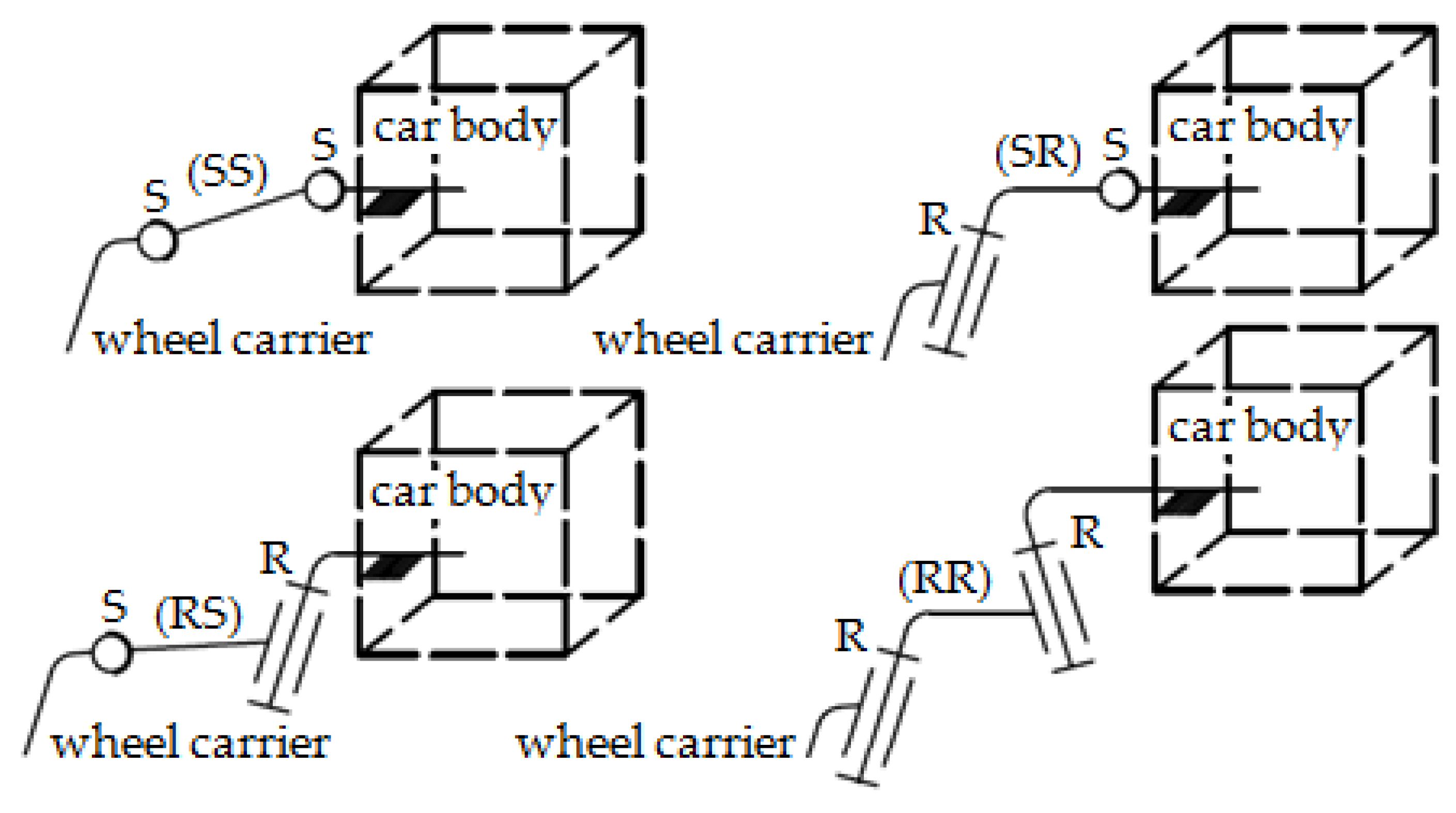
From a kinematic point of view, the guidance mechanism must ensure the vertical movement (travel) of the wheel, so the required degree of mobility is M = 1. In order to obtain such mono-mobile mechanisms, various structural synthesis methods are presented in the literature, depending on the type of mechanism, the number of guidance points on the wheel carrier and chassis, and the type and number of kinematic chains interspersed between these parts [8]. The need to obtain simple and safe guidance mechanisms has led to the use of the types of guidance shown in Figure 1, with a large variety of wheel guidance mechanisms (some of which are used in practice) being obtainable by connecting/combining these basic chains.

The dynamic model of the wheel suspension system is obtained by completing the structural model with the mass and inertia properties of the component bodies, the arrangement parameters and characteristics of the elastic and damping elements, and the external forces acting on the car, depending on the specific running mode.

Under the action of external forces and the reaction forces in the system, the suspension mechanism will occupy a certain position in relation to the chassis, called the equilibrium (balance) position. Establishing this position is necessary to assess the behavior of the vehicle in various operating/loading regimes, and to determine the reactions in joints in order to properly size them. Such a problem is approached in the literature mainly using energetic methods, based on the minimum energy potential in the equilibrium position, or by kinetostatic analysis methods, decomposing the suspension mechanism into components and expressing their equilibrium equations [9,10,11,12,13,14,15,16]. The equilibrium position can also be determined by using automatic analysis algorithms, which are integrated in the commercial MBS (Multi-Body Systems) software environments, such as ADAMS, DYMES, or SIMPACK. These virtual prototyping tools provide important benefits in the simulation and optimization of the mechanical and mechatronic systems, but their high cost and the need for effective training are still limiting factors [17,18,19,20].

This paper deals with an analytical method for determining the equilibrium position of the non-steered wheel suspension systems, which is based on the virtual mechanical work principle [21,22]. An algorithm for the analysis of relative movements in the guidance mechanism is developed, with the purpose of determining the deformations (and subsequently the reaction forces) in the elastic elements. Not only the methods themselves but also the mode in which they are integrated in a unitary algorithm are elements of originality.

This paper actually continues a previous study [23], which dealt with a method for the quasi-static analysis of beam axle suspension, a dependent suspension design in which the set of two wheels is connected laterally by a single beam. Unlike this, the current work is about independent wheel suspension systems, where each wheel has its own suspension mechanism relative to the chassis. Beam axle suspension is commonly used for light commercial and off-road vehicles while the solution addressed in this work is intended primarily for passenger cars.

2. Forces Acting on the Car

As a premise for the study developed in this paper, the car is considered as a rigid body, on which a complex group of forces acts [24,25]. The loading scheme in the general case of overlapping operating modes (car turning on a sloping and transversely inclined road) is shown in Figure 2, according to which the following can be determined:

• The weight force (G_a), with the point of application in the center of mass O_c of the car:

  $${\mathrm{G}}_{\mathrm{a}}\hspace{0.17em}=\hspace{0.17em}{\mathrm{G}}_{\mathrm{o}}\hspace{0.17em}+\hspace{0.17em}{\mathrm{G}}_{\mathrm{s}}\hspace{0.17em}+\hspace{0.17em}{\mathrm{G}}_{\mathrm{i}},$$

  (1)

  where G_o is the empty car weight, G_s is the driver weight, and G_i is the cargo weight (the load state will be considered, as the case may be, G_o, G_o + G_s, or G_o + G_s + G_i, respectively);
• The centrifugal force (F_c), applied in O_c, in the direction of the turning radius r_c and the positive direction to the outside of the turn:

  $${\mathrm{F}}_{\mathrm{c}}\hspace{0.17em}=\hspace{0.17em}\frac{{\mathrm{m}}_{\mathrm{a}}\hspace{0.17em}\cdot \hspace{0.17em}{\mathrm{v}}_{\mathrm{a}}^2}{{\mathrm{r}}_{\mathrm{c}}},$$

  (2)

  where m_a is the mass of the car, and v_a is the travel speed;
• The air resistance (drag) forces (F_ax, F_ay), which are applied relative to the ground level at the height h_a (in the center of pressure, for the determination of which complex experimental and CFD tests are required) [26], or h_c (in the center of gravity, as a main simplification), with a positive direction opposite to the X, Y axes:

  $${\mathrm{F}}_{\mathrm{ax}}=0.5\cdot \mathsf{\rho }\cdot {\mathrm{k}}_{\mathrm{ax}}\cdot {\mathrm{S}}_{\mathrm{x}}\hspace{0.17em}\cdot { \mathrm{v}}_{\mathrm{ax}}^2,\hspace{0.17em}{\mathrm{F}}_{\mathrm{ay}}=0.5\cdot \hspace{0.17em}\mathsf{\rho }\cdot {\mathrm{k}}_{\mathrm{ay}}\cdot {\mathrm{S}}_{\mathrm{y}}\hspace{0.17em}\cdot { \mathrm{v}}_{\mathrm{ay}}^2,$$

  (3)

  where ρ is the air density, k_ax is the frontal aerodynamic drag coefficient, k_ay is the lateral aerodynamic drag coefficient, S_x is the frontal area of the car along the X direction, S_y is the lateral area along the Y direction, v_ax is the vehicle speed along X, and v_ay is the vehicle speed along Y (when skidding) [27];
• The resistance forces to acceleration/inertia-longitudinal (traction or braking), lateral (skidding) and vertical (crossing obstacles), along the directions of the axes and positive direction along the Y axis, respectively, opposite the X, Z axes (F_dx, F_dy, F_dz):

  $${\mathrm{F}}_{\mathrm{dx}}{=\mathrm{k}}_{\mathrm{x}}\cdot {\mathrm{G}}_{\mathrm{a}}{, \mathrm{F}}_{\mathrm{dy}}{=\mathrm{k}}_{\mathrm{y}}\cdot {\mathrm{G}}_{\mathrm{a}}{, \mathrm{F}}_{\mathrm{dz}}{=\mathrm{k}}_{\mathrm{z}}\cdot {\mathrm{G}}_{\mathrm{a}},$$

  (4)

  where k_x, k_y, and k_z are the acceleration coefficients, with positive values for accelerated traction (k_x > 0), skidding to the left (k_y > 0), and accelerated jump over obstacles (k_z > 0);
• The torque of wheel inertia forces (${\mathrm{M}}_{\mathrm{r}}^{\mathrm{i}}$), having the direction of the wheels’ axles and the positive direction towards the turning center O_v:

  $${\mathrm{M}}_{\mathrm{r}}^{\mathrm{i}}\hspace{0.17em}=\hspace{0.17em}\frac{{\mathrm{J}}_{\mathrm{r}}\hspace{0.17em}\cdot \hspace{0.17em}{\mathrm{k}}_{\mathrm{x}}\hspace{0.17em}\cdot \hspace{0.17em}\mathrm{g}}{\mathrm{r}},$$

  (5)

  for each of the four wheels, where J_r is the wheel inertia torque and r is the wheel radius.

These forces, which depend on the loading and driving regime of the car, are transmitted to the ground by means of the suspension and the wheels, being balanced by the reactions that appear at the tire–road contact, as follows:

• Normal reactions (Z_A, Z_B, Z_C, Z_D), which are normally arranged on the running surface;
• Tangential reactions at the drive (motor) axle (X_A, X_B), as ground adhesion forces, or at the non-motor axle (X_C, X_D), as ground friction forces:

  $${\mathrm{X}}_{\mathrm{A},\mathrm{B}}={\mathsf{\Psi }}_{\mathrm{a}}\cdot {\mathrm{Z}}_{\mathrm{A},\mathrm{B}},{ \mathrm{X}}_{\mathrm{C},\mathrm{D}}{=\mathrm{f}}_{\mathrm{r}}\cdot {\mathrm{Z}}_{\mathrm{C},\mathrm{D}},$$

  (6)

  or when braking:

  $${\mathrm{X}}_{\mathrm{C},\mathrm{D}}={\mathsf{\Psi }}_{\mathrm{a}}\cdot {\mathrm{Z}}_{\mathrm{C},\mathrm{D}},$$

  (7)

  where Ψ_a is the adhesion coefficient [28] and f_r is the rolling resistance coefficient [29];
• Lateral reactions (Y_A, Y_B, Y_C, Y_D), as skidding resistance forces:

  $${\mathrm{Y}}_{\mathrm{A},\hspace{0.17em}\mathrm{B},\hspace{0.17em}\mathrm{C},\hspace{0.17em}\mathrm{D}}={\mathsf{\mu }}_{\mathrm{l}}\cdot {\mathrm{Z}}_{\mathrm{A},\hspace{0.17em}\mathrm{B},\hspace{0.17em}\mathrm{C},\hspace{0.17em}\mathrm{D}},$$

  (8)

  where μ_l is the lateral friction coefficient [30];
• Rolling resistance torques of the front and rear wheels (${\mathrm{M}}_{\mathrm{A}}^{\mathrm{r}},\hspace{0.17em}{\mathrm{M}}_{\mathrm{B}}^{\mathrm{r}},\hspace{0.17em}{\mathrm{M}}_{\mathrm{C}}^{\mathrm{r}},\hspace{0.17em}{\mathrm{M}}_{\mathrm{D}}^{\mathrm{r}}$):

  $${\mathrm{M}}_{\mathrm{A},\hspace{0.17em}\mathrm{B},\hspace{0.17em}\mathrm{C},\hspace{0.17em}\mathrm{D}}^{\mathrm{r}}{=\mathrm{f}}_{\mathrm{r}}\cdot \hspace{0.17em}\mathrm{r}\hspace{0.17em}\cdot {\mathrm{Z}}_{\mathrm{A},\hspace{0.17em}\mathrm{B},\hspace{0.17em}\mathrm{C},\hspace{0.17em}\mathrm{D}}$$

  (9)

The unknowns in the previous equations are the normal reactions to the wheels (Z_A, Z_B, Z_C, Z_D), which result from the overall balance of the car, by overlapping effects [24,25]. In this regard, the road on which the car moves is tilted both longitudinally (angle α_c in Figure 2) and transversely (angle β_c). The car is cornering at angle θ_f, with respect to the driving radius r_c from the center of mass O_c. Subsequently, the tangential and lateral reactions are obtained from Equations (6)/(7) and (8).

3. Algorithm for Finding the Static Equilibrium

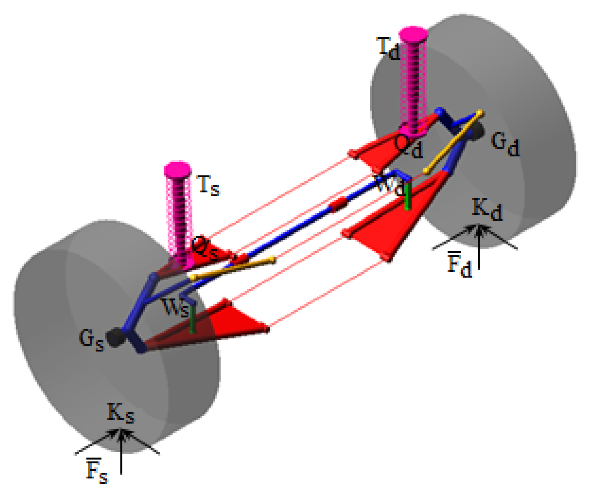
The equilibrium configuration of the suspension system in relation to the car body (considered as the fixed reference part) is determined on the static model (Figure 3), which is defined by kinematic elements (bodies), geometric constraints (joints), and elastic elements. Determining the equilibrium configuration consists in establishing the independent positional parameter (the wheel guidance mechanisms having one degree of mobility), which corresponds to the vertical displacement of the wheel center (Z_Gs or Z_Gd).

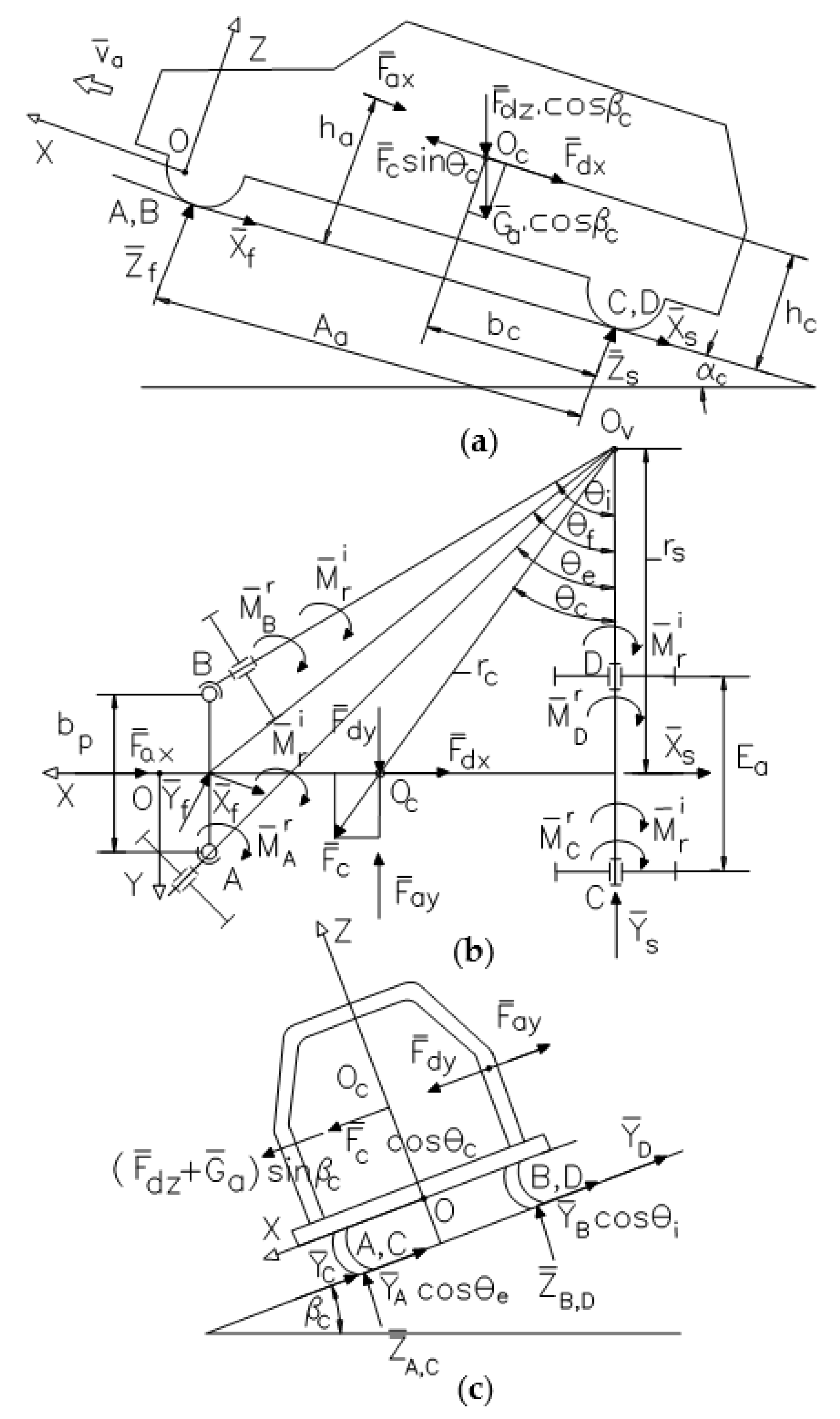
The external loading of the suspension system is carried out by forces applied to the wheels (F_s,d), in the theoretical contact point with the ground (K_s,d), corresponding to the specific operating regime (such as stationary, traction, braking, skidding). These are balanced by the reaction forces or torques in the elastic elements of the suspension system, as follows:

• The forces in the springs (F_as,d), which are applied in Q_s,d;
• The torsional (M_ft) and conical (M_fc) torques in the bushings (which are modeled by spherical joints, with elastically restricted rotations);
• The forces in the buffers for limiting the suspension travel (F_ts,d), which are applied in T_s,d;
• The forces in the anti-roll bar (F_ws,d), which are applied in the connection points W_s,d of the anti-roll bar to the connecting rods.

With the exception of the forces in the anti-roll bar, which depend on both independent parameters (i.e., the vertical coordinates of the wheels’ centers, Z_Gs and Z_Gd), the other elastic forces depend only on the parameter corresponding to the left or right side of the suspension (by case, Z_Gs or Z_Gd).

It must be noted that due to the anti-roll bar, which is connected between parts from the left and right guidance mechanisms, it is necessary to consider the transverse half-car model of the suspension system (such as the one shown in Figure 3, where the anti-roll bar is connected by rods to the lower guidance arms), which considers the suspension systems of both axle wheels, and not just the quarter-car model corresponding to the suspension of a single wheel [31,32,33].

Although, under the action of wheel reaction forces, not only do the elastic elements of the suspension deform but so do the tires and sometimes even the bars of the guidance mechanism. These deformations are not taken into account in the determination of the equilibrium position, which considers them negligible compared to the deformation of the suspension elements. It should be mentioned that in the automotive industry, there are some experimental tests carried out on a so-called full-vehicle road simulator (test rig), in which the wheels are disassembled/removed, and the external forces are applied (by some actuators) directly to the wheel spindle level [34]. Such an actuating mode is largely equivalent to the “rigid tire” assumption used in this work. Therefore, the mechanical work developed by the wheel reaction forces is transformed only into mechanical work of deformation of the elastic elements of the suspension.

According to the principle of virtual mechanical work, the sum of the virtual works performed by the wheel reaction forces and the specified elastic balancing forces/torques, for any virtual movement compatible with the connections, is equal to zero:

$${\mathrm{F}}_{\mathrm{s}}\cdot \hspace{0.17em}\mathsf{\delta }{\mathrm{r}}_{\mathrm{Ks}}{+\mathrm{F}}_{\mathrm{d}}\cdot \hspace{0.17em}\mathsf{\delta }{\mathrm{r}}_{\mathrm{Kd}}{+\mathrm{F}}_{\mathrm{as}}\cdot \hspace{0.17em}\mathsf{\delta }{\mathrm{r}}_{\mathrm{Qs}}{+\mathrm{F}}_{\mathrm{ad}}\cdot \hspace{0.17em}\mathsf{\delta }{\mathrm{r}}_{\mathrm{Qd}}{+\mathrm{F}}_{\mathrm{ts}}\cdot \hspace{0.17em}\mathsf{\delta }{\mathrm{r}}_{\mathrm{Ts}}{+\mathrm{F}}_{\mathrm{td}}\cdot \hspace{0.17em}\mathsf{\delta }{\mathrm{r}}_{\mathrm{Td}}{+\mathrm{F}}_{\mathrm{ws}}\cdot \hspace{0.17em}\mathsf{\delta }{\mathrm{r}}_{\mathrm{Ws}}{+\mathrm{F}}_{\mathrm{wd}}\cdot {\mathsf{\delta }\mathrm{r}}_{\mathrm{Wd}}+{\displaystyle \sum _{\mathrm{i}=1}^{\mathrm{n}}{\left({\mathrm{M}}_{\mathrm{f}}\hspace{0.17em}\cdot \hspace{0.17em}\mathsf{\delta }{\mathsf{\varphi }}_{\mathrm{r}}\right)}_{\mathrm{i}}}=0\hspace{0.17em},$$

(10)

where “n” is the number of bushings by which the guidance bars are connected to the adjacent parts (car body and wheel carrier, respectively).

The magnitude of the elastic forces and torques depends on the deformations of the elastic elements and their stiffness coefficients, with the computation mode being similar to that depicted in [35]. The deformations result from the spatial position and orientation of the suspension mechanism relative to the car body, which is defined by the generalized coordinates Z_Gs and Z_Gd (detailed in Section 4).

For springs, bushings, and buffers, the virtual linear (δr) and angular (δϕ) displacements are expressed according to the generalized coordinate from the corresponding suspension side (Z_Gs or Z_Gd, by case):

$$\mathsf{\delta }\mathrm{r}\hspace{0.17em}=\hspace{0.17em}\mathsf{\delta }\mathrm{r}\left({\mathrm{Z}}_{\mathrm{G}\mathrm{s}\hspace{0.17em}/\mathrm{G}\mathrm{d}}\right)\hspace{0.17em}=\hspace{0.17em}\frac{\mathsf{\upsilon }\mathrm{r}}{\mathsf{\upsilon }{\mathrm{Z}}_{\mathrm{G}\mathrm{s}\hspace{0.17em}/\hspace{0.17em}\mathrm{G}\mathrm{d}}}\hspace{0.17em}\cdot \hspace{0.17em}\mathsf{\delta }{\mathrm{Z}}_{\mathrm{G}\mathrm{s}\hspace{0.17em}/\hspace{0.17em}\mathrm{G}\mathrm{d}},\hspace{0.17em}\mathsf{\delta }\mathsf{\varphi }\hspace{0.17em}=\hspace{0.17em}\mathsf{\delta }\mathsf{\varphi }\left({\mathrm{Z}}_{\mathrm{G}\mathrm{s}\hspace{0.17em}/\hspace{0.17em}\mathrm{G}\mathrm{d}}\right)\hspace{0.17em}=\hspace{0.17em}\frac{\mathsf{\upsilon }\mathsf{\varphi }}{\mathsf{\upsilon }{\mathrm{Z}}_{\mathrm{G}\mathrm{s}\hspace{0.17em}/\hspace{0.17em}\mathrm{G}\mathrm{d}}}\hspace{0.17em}\cdot \hspace{0.17em}\mathsf{\delta }{\mathrm{Z}}_{\mathrm{G}\mathrm{s}\hspace{0.17em}/\hspace{0.17em}\mathrm{G}\mathrm{d}}.$$

(11)

while for the anti-roll bar, both coordinates influence the virtual displacements:

$$\mathsf{\delta }{\mathrm{r}}_{\mathrm{W}\mathrm{s}/\mathrm{W}\mathrm{d}}\hspace{0.17em}=\hspace{0.17em}\mathsf{\delta }{\mathrm{r}}_{\mathrm{W}\mathrm{s}/\mathrm{W}\mathrm{d}}\left({\mathrm{Z}}_{\mathrm{G}\mathrm{s}},\hspace{0.17em}{\mathrm{Z}}_{\mathrm{G}\mathrm{d}}\right)\hspace{0.17em}=\hspace{0.17em}\frac{\mathsf{\upsilon }{\mathrm{r}}_{\mathrm{W}\mathrm{s}/\mathrm{W}\mathrm{d}}}{\mathsf{\upsilon }{\mathrm{Z}}_{\mathrm{G}\mathrm{s}}}\hspace{0.17em}\cdot \hspace{0.17em}\mathsf{\delta }{\mathrm{Z}}_{\mathrm{G}\mathrm{s}}\hspace{0.17em}+\hspace{0.17em}\frac{\mathsf{\upsilon }{\mathrm{r}}_{\mathrm{W}\mathrm{s}/\mathrm{W}\mathrm{d}}}{\mathsf{\upsilon }{\mathrm{Z}}_{\mathrm{G}\mathrm{d}}}\hspace{0.17em}\cdot \hspace{0.17em}\mathsf{\delta }{\mathrm{Z}}_{\mathrm{G}\mathrm{d}}.$$

(12)

Each of the two (left and right) wheel guidance mechanisms has one degree of mobility (i.e., the vertical displacement/travel of the related wheel), with the equation of virtual mechanical work (10) being transposed into a two-equation nonlinear system as follows:

$$\begin{array}{l}{\mathrm{F}}_1\left({\mathrm{Z}}_{\mathrm{Gs}},\hspace{0.17em}{\mathrm{Z}}_{\mathrm{Gd}}\right)={\mathrm{F}}_{\mathrm{s}}\cdot \frac{{\mathsf{\upsilon }\mathrm{r}}_{\mathrm{Ks}}}{{\mathsf{\upsilon }\mathrm{Z}}_{\mathrm{Gs}}}+{\mathrm{F}}_{\mathrm{as}}\cdot \frac{{\mathsf{\upsilon }\mathrm{r}}_{\mathrm{Qs}}}{{\mathsf{\upsilon }\mathrm{Z}}_{\mathrm{Gs}}}\hspace{0.17em}+\hspace{0.17em}{\mathrm{F}}_{\mathrm{ts}}\cdot \frac{{\mathsf{\upsilon }\mathrm{r}}_{\mathrm{Ts}}}{{\mathsf{\upsilon }\mathrm{Z}}_{\mathrm{Gs}}}+{\mathrm{F}}_{\mathrm{ws}}\cdot \frac{{\mathsf{\upsilon }\mathrm{r}}_{\mathrm{Ws}}}{{\mathsf{\upsilon }\mathrm{Z}}_{\mathrm{Gs}}}+{\mathrm{F}}_{\mathrm{ws}}\cdot \frac{{\mathsf{\upsilon }\mathrm{r}}_{\mathrm{Ws}}}{{\mathsf{\upsilon }\mathrm{Z}}_{\mathrm{Gd}}}+\hspace{0.17em}{\displaystyle \sum _{\mathrm{i}=1}^{\mathrm{n}}{\left({\mathrm{M}}_{\mathrm{F}}\cdot \frac{\mathsf{\upsilon }\mathsf{\varphi }}{{\mathsf{\upsilon }\mathrm{Z}}_{\mathrm{Gs}}}\right)}_{\mathrm{i}}=0,}\\ {\mathrm{F}}_2\left({\mathrm{Z}}_{\mathrm{Gs}},\hspace{0.17em}{\mathrm{Z}}_{\mathrm{Gd}}\right)={\mathrm{F}}_{\mathrm{d}}\cdot \frac{{\mathsf{\upsilon }\mathrm{r}}_{\mathrm{Kd}}}{{\mathsf{\upsilon }\mathrm{Z}}_{\mathrm{Gd}}}+{\mathrm{F}}_{\mathrm{ad}}\cdot \frac{{\mathsf{\upsilon }\mathrm{r}}_{\mathrm{Qd}}}{{\mathsf{\upsilon }\mathrm{Z}}_{\mathrm{Gd}}}+{\mathrm{F}}_{\mathrm{td}}\cdot \frac{{\mathsf{\upsilon }\mathrm{r}}_{\mathrm{Td}}}{{\mathsf{\upsilon }\mathrm{Z}}_{\mathrm{Gd}}}+{\mathrm{F}}_{\mathrm{wd}}\cdot \frac{{\mathsf{\upsilon }\mathrm{r}}_{\mathrm{Wd}}}{{\mathsf{\upsilon }\mathrm{Z}}_{\mathrm{Gs}}}+{\mathrm{F}}_{\mathrm{wd}}\cdot \frac{{\mathsf{\upsilon }\mathrm{r}}_{\mathrm{Wd}}}{{\mathsf{\upsilon }\mathrm{Z}}_{\mathrm{Gd}}}+{\displaystyle \sum _{\mathrm{i}=1}^{\mathrm{n}}{\left({\mathrm{M}}_{\mathrm{F}}\cdot \frac{\mathsf{\upsilon }\mathsf{\varphi }}{{\mathsf{\upsilon }\mathrm{Z}}_{\mathrm{Gd}}}\right)}_{\mathrm{i}}=0.}\end{array}$$

(13)

Determining the equilibrium position is further reduced to a mono-objective optimal design problem (without design constraints), which consists of determining the values of the independent design variables Z_Gs and Z_Gd, for which the function:

$$\mathrm{F}\left({\mathrm{Z}}_{\mathrm{Gs}},\hspace{0.17em}{\mathrm{Z}}_{\mathrm{G}\mathrm{d}}\right)\hspace{0.17em}=\left|{\mathrm{F}}_1\left({\mathrm{Z}}_{\mathrm{Gs}},\hspace{0.17em}{\mathrm{Z}}_{\mathrm{Gd}\hspace{0.17em}}\right)\right|\hspace{0.17em}+\hspace{0.17em}\left|{\mathrm{F}}_2\left({\mathrm{Z}}_{\mathrm{Gs}},\hspace{0.17em}{\mathrm{Z}}_{\mathrm{Gd}\hspace{0.17em}}\right)\right|,\hspace{0.17em}\hspace{0.17em}{\mathrm{Z}}_{\mathrm{Gs},\hspace{0.17em}\mathrm{d}}\hspace{0.17em}\in \hspace{0.17em}\left[{\mathrm{Z}}_{\mathrm{Gs},\hspace{0.17em}\mathrm{d} \min },\hspace{0.17em}{\mathrm{Z}}_{\mathrm{Gs},\hspace{0.17em}\mathrm{d} \max }\right],$$

(14)

has a minimum value. The solution can be determined through an iterative process by considering discrete values for the two design variables in the compression (up)–extension (down) operating range of the suspension mechanism, and by identifying the values that ensure the minimum of the function (14).

The value pairs for the design variables were generated through the next sequence:

$$\begin{array}{l}{\mathrm{Z}}_{\mathrm{Gs}}^0\hspace{0.17em}=\hspace{0.17em}{\mathrm{Z}}_{\mathrm{Gs}\hspace{0.17em}\min },\hspace{0.17em}{\mathrm{Z}}_{\mathrm{Gd}}\hspace{0.17em}\in \hspace{0.17em}\left[{\mathrm{Z}}_{\mathrm{Gd}\hspace{0.17em}\min },\hspace{0.17em}{\mathrm{Z}}_{\mathrm{Gd}\hspace{0.17em}\max }\right],\\ {\mathrm{Z}}_{\mathrm{Gs}}^1\hspace{0.17em}=\hspace{0.17em}{\mathrm{Z}}_{\mathrm{Gs}}^0\hspace{0.17em}+\hspace{0.17em}\mathrm{\Delta }{\mathrm{Z}}_{\mathrm{Gs}},\hspace{0.17em}{\mathrm{Z}}_{\mathrm{Gd}}\hspace{0.17em}\in \hspace{0.17em}\left[{\mathrm{Z}}_{\mathrm{Gd}\hspace{0.17em}\min },\hspace{0.17em}{\mathrm{Z}}_{\mathrm{Gd}\hspace{0.17em}\max }\right],\\ \dots \\ {\mathrm{Z}}_{\mathrm{Gs}}^{\mathrm{k}+1}\hspace{0.17em}=\hspace{0.17em}{\mathrm{Z}}_{\mathrm{Gs}}^{\mathrm{k}}\hspace{0.17em}+\hspace{0.17em}\Delta {\mathrm{Z}}_{\mathrm{Gs}},\hspace{0.17em}{\mathrm{Z}}_{\mathrm{Gd}}\hspace{0.17em}\in \hspace{0.17em}\left[{\mathrm{Z}}_{\mathrm{Gd}\hspace{0.17em}\min },\hspace{0.17em}{\mathrm{Z}}_{\mathrm{Gd}\hspace{0.17em}\max }\right],\\ \dots \\ {\mathrm{Z}}_{\mathrm{Gs}}\hspace{0.17em}=\hspace{0.17em}{\mathrm{Z}}_{\mathrm{Gs}\hspace{0.17em}\max },\hspace{0.17em}{\mathrm{Z}}_{\mathrm{Gd}}\hspace{0.17em}\in \hspace{0.17em}\left[{\mathrm{Z}}_{\mathrm{Gd}\hspace{0.17em}\min },\hspace{0.17em}{\mathrm{Z}}_{\mathrm{Gd}\hspace{0.17em}\max }\right],\end{array}$$

(15)

where ΔZ_Gs is the step by which the design variable Z_Gs changes (similarly, the other design variable, Z_Gd, changes with the step ΔZ_Gd within its own variation range).

In each iteration, the position of the suspension mechanism in relation to the car body, the reduced speeds, the deformations of the elastic elements and their reaction forces, and the corresponding value of the objective function are determined. The iterative process is completed when the objective function becomes small enough:

$$\mathrm{F}\left({\mathrm{Z}}_{\mathrm{Gs}},\hspace{0.17em}{\mathrm{Z}}_{\mathrm{Gd}}\right) \le \hspace{0.17em}\mathsf{\epsilon },$$

(16)

where ε is the admissible error (it was considered ε = 0.001).

The process of determining the optimal solution could be favored by the use of automated search algorithms, for example, the Hook–Jeeves method [36], thus reducing the computation time.

If there is no anti-roll bar, or if the external forces on the left and right wheels are equal (so the anti-roll bar does not operate), the Equation (13) can be solved independently, in the following form:

$$\begin{array}{l}{\mathrm{F}}_1\left({\mathrm{Z}}_{\mathrm{Gs}}\right)={\mathrm{F}}_{\mathrm{s}}\cdot \frac{{\mathsf{\upsilon }\mathrm{r}}_{\mathrm{Ks}}}{{\mathsf{\upsilon }\mathrm{Z}}_{\mathrm{Gs}}}+{\mathrm{F}}_{\mathrm{as}}\cdot \frac{{\mathsf{\upsilon }\mathrm{r}}_{\mathrm{Qs}}}{{\mathsf{\upsilon }\mathrm{Z}}_{\mathrm{Gs}}}\hspace{0.17em}+\hspace{0.17em}{\mathrm{F}}_{\mathrm{ts}}\cdot \frac{{\mathsf{\upsilon }\mathrm{r}}_{\mathrm{Ts}}}{{\mathsf{\upsilon }\mathrm{Z}}_{\mathrm{Gs}}}+{\mathrm{F}}_{\mathrm{ws}}\cdot \frac{{\mathsf{\upsilon }\mathrm{r}}_{\mathrm{Ws}}}{{\mathsf{\upsilon }\mathrm{Z}}_{\mathrm{Gs}}}+\hspace{0.17em}{\displaystyle \sum _{\mathrm{i}=1}^{\mathrm{n}}{\left({\mathrm{M}}_{\mathrm{f}}\cdot \frac{\mathsf{\upsilon }\mathsf{\phi }}{{\mathsf{\upsilon }\mathrm{Z}}_{\mathrm{Gs}}}\right)}_{\mathrm{i}}=0,}\\ {\mathrm{F}}_2\left({\mathrm{Z}}_{\mathrm{Gd}}\right)={\mathrm{F}}_{\mathrm{d}}\cdot \frac{{\mathsf{\upsilon }\mathrm{r}}_{\mathrm{Kd}}}{{\mathsf{\upsilon }\mathrm{Z}}_{\mathrm{Gd}}}+{\mathrm{F}}_{\mathrm{ad}}\cdot \frac{{\mathsf{\upsilon }\mathrm{r}}_{\mathrm{Qd}}}{{\mathsf{\upsilon }\mathrm{Z}}_{\mathrm{Gd}}}+{\mathrm{F}}_{\mathrm{td}}\cdot \frac{{\mathsf{\upsilon }\mathrm{r}}_{\mathrm{Td}}}{{\mathsf{\upsilon }\mathrm{Z}}_{\mathrm{Gd}}}+{\mathrm{F}}_{\mathrm{wd}}\cdot \frac{{\mathsf{\upsilon }\mathrm{r}}_{\mathrm{Wd}}}{{\mathsf{\upsilon }\mathrm{Z}}_{\mathrm{Gd}}}+{\displaystyle \sum _{\mathrm{i}=1}^{\mathrm{n}}{\left({\mathrm{M}}_{\mathrm{f}}\cdot \frac{\mathsf{\upsilon }\mathsf{\phi }}{{\mathsf{\upsilon }\mathrm{Z}}_{\mathrm{Gd}}}\right)}_{\mathrm{i}}=0.}\end{array}$$

(17)

which obviously leads to simplification of the calculation, with the two objective functions having to be minimized separately, by searching for the optimal value of a single design variable (Z_Gs or Z_Gd, as the case may be), as follows:

$${\mathrm{F}}_1\left({\mathrm{Z}}_{\mathrm{Gs}}\right) \le \hspace{0.17em}\mathsf{\epsilon },\hspace{0.17em}{\mathrm{F}}_2\left({\mathrm{Z}}_{\mathrm{Gd}}\right) \le \hspace{0.17em}\mathsf{\epsilon }.$$

(18)

In the situation where by completing the iterative process (15), no solution is identified (as values of the generalized coordinates Z_Gs and/or Z_Gd) that satisfies the requirement (16) or (18), as the case may be, the process is resumed from the beginning by modifying the variation step of the generalized coordinate(s) (ΔZ_Gs/d), in the sense of reducing it (thus, increasing the accuracy of finding the optimal solution).

The method described in the next section of the paper was used for the positional (kinematic) analysis of the non-steered wheel guidance mechanisms, as part of the general algorithm for finding the static equilibrium of the suspension system.

4. Kinematic Analysis of the Wheel Guidance Mechanisms

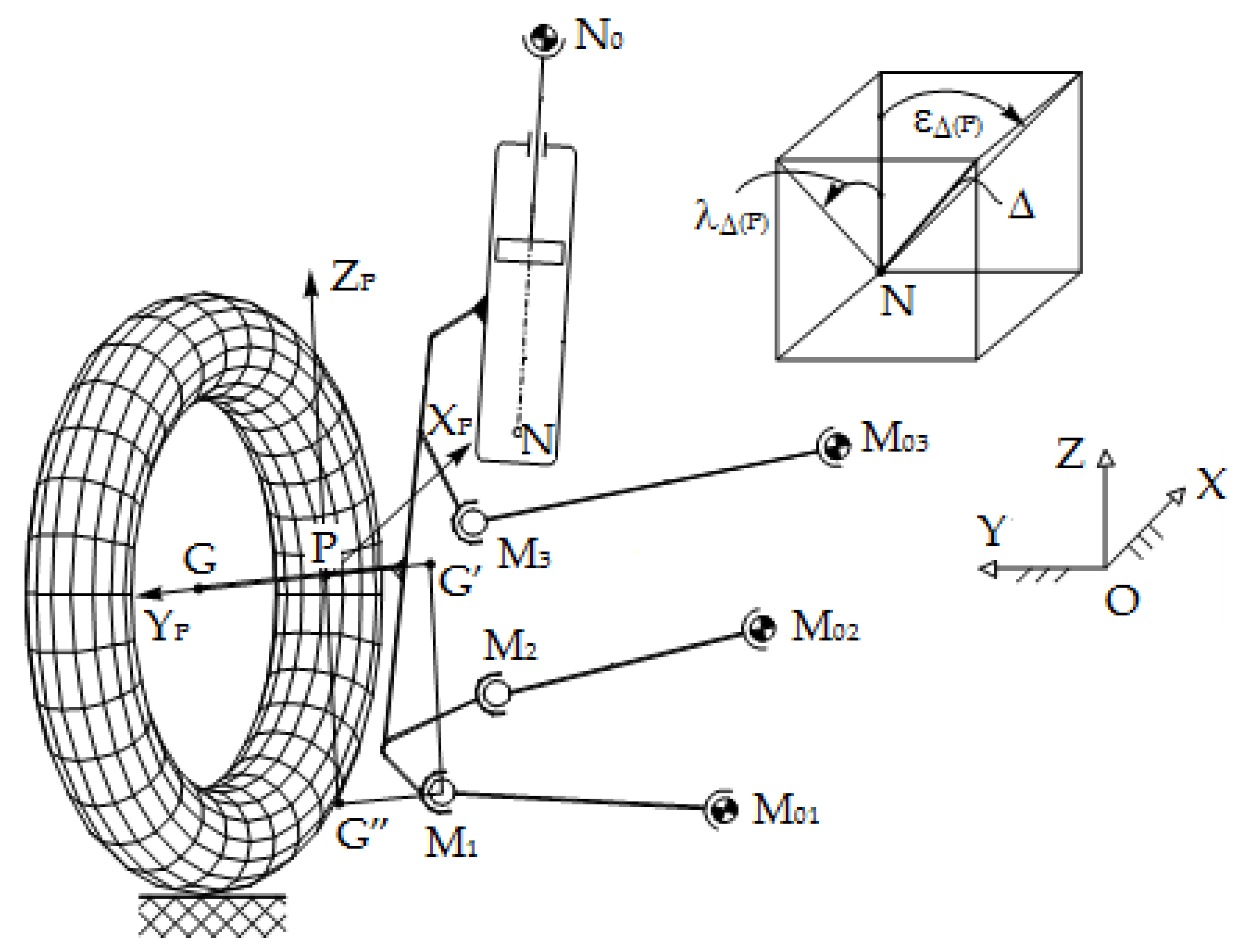
The current spatial position and orientation of the wheel, relative to the global reference frame attached to the car body (OXYZ), is completely determined by three non-collinear characteristic points (see Figure 4): the center G of the wheel (G_s/d for the left/right wheel), and the projections G′, G″ of the lower guidance point M₁ on the transverse and vertical axes of the wheel carrier reference frame (PX_PY_PZ_P).

The axes of the global reference frame OXYZ are directed in parallel to the car’s axles (with the positive X-axis towards the front of the car, the positive Y-axis towards the left, and the positive Z-axis upwards), where the origin O is located at the intersection of the median longitudinal–vertical and vertical–transversal plans. The wheel carrier reference frame PX_PY_PZ_P has the origin P in the center of the spindle axis, along which the local transverse axis Y_P is directed.

The system of position functions for determining the global coordinates of the three points defining the local frame includes the condition that the distances between these points are constant (given that the wheel carrier is a rigid body) and the constraints imposed on the points M_i by which the wheel carrier is guided, as follows:

$$\begin{array}{l}{\mathrm{F}}_1\hspace{0.17em}=\hspace{0.17em}{\left({\mathrm{X}}_{{\mathrm{G}}^{″}}{ - \mathrm{X}}_{{\mathrm{G}}^{\prime }}\right)}^2+{\left({\mathrm{Y}}_{{\mathrm{G}}^{″}}{ - \mathrm{Y}}_{{\mathrm{G}}^{\prime }}\right)}^2+{\left({\mathrm{Z}}_{{\mathrm{G}}^{″}}{ - \mathrm{Z}}_{{\mathrm{G}}^{\prime }}\right)}^2{ - {\mathrm{G}}^{″}{\mathrm{G}}^{\prime }}^2=0,\\ {\mathrm{F}}_2\hspace{0.17em}=\hspace{0.17em}{\left({\mathrm{X}}_{{\mathrm{G}}^{″}}{ - \mathrm{X}}_{\mathrm{G}}\right)}^2+{\left({\mathrm{Y}}_{{\mathrm{G}}^{″}}{ - \mathrm{Y}}_{\mathrm{G}}\right)}^2+{\left({\mathrm{Z}}_{{\mathrm{G}}^{″}}{ - \mathrm{Z}}_{\mathrm{G}}\right)}^2{ - {\mathrm{G}}^{″}\mathrm{G}}^2=0,\\ {\mathrm{F}}_3\hspace{0.17em}=\hspace{0.17em}{\left({\mathrm{X}}_{{\mathrm{G}}^{\prime }}{ - \mathrm{X}}_{\mathrm{G}}\right)}^2+{\left({\mathrm{Y}}_{{\mathrm{G}}^{\prime }}{ - \mathrm{Y}}_{\mathrm{G}}\right)}^2+{\left({\mathrm{Z}}_{{\mathrm{G}}^{\prime }}{ - \mathrm{Z}}_{\mathrm{G}}\right)}^2{ - {\mathrm{G}}^{\prime }\mathrm{G}}^2=0,\\ {\mathrm{F}}_{\mathrm{i}}\hspace{0.17em}=\hspace{0.17em}{\left({\mathrm{X}}_{\mathrm{Mi}}{ - \mathrm{X}}_{\mathrm{M}0\mathrm{i}}\right)}^2+{\left({\mathrm{Y}}_{\mathrm{Mi}}{ - \mathrm{Y}}_{\mathrm{M}0\mathrm{i}}\right)}^2+{\left({\mathrm{Z}}_{\mathrm{Mi}}{ - \mathrm{Z}}_{\mathrm{M}0\mathrm{i}}\right)}^2{ - \mathrm{l}}_{\mathrm{i}}^2=0.\end{array}$$

(19)

The guidance on the circle of the point M_i (e.g., the guidance arm 1 in Figure 4) introduces two equations of the form F_i in Equation (19), namely the pairs ${\mathrm{M}}_{\mathrm{i}}\hspace{0.17em}-\hspace{0.17em}{\mathrm{M}}_{0\mathrm{i}}^{\prime }$ and ${\mathrm{M}}_{\mathrm{i}}\hspace{0.17em}-\hspace{0.17em}{\mathrm{M}}_{0\mathrm{i}}^{"}$.

The global coordinates of the guidance points Mi are determined according to the positions of the points G, G′, and G″, as follows:

$$\left[\begin{array}{c}{\mathrm{X}}_{\mathrm{Mi}}\\ {\mathrm{Y}}_{\mathrm{Mi}}\\ {\mathrm{Z}}_{\mathrm{Mi}}\end{array}\right]=\left[\begin{array}{c}{\mathrm{X}}_{\mathrm{P}}\\ {\mathrm{Y}}_{\mathrm{P}}\\ {\mathrm{Z}}_{\mathrm{P}}\end{array}\right]+\left[\begin{array}{ccc}{\mathrm{a}}_{11}& {\mathrm{a}}_{12}& {\mathrm{a}}_{13}\\ {\mathrm{a}}_{21}& {\mathrm{a}}_{22}& {\mathrm{a}}_{23}\\ {\mathrm{a}}_{31}& {\mathrm{a}}_{32}& {\mathrm{a}}_{33}\end{array}\right]\cdot {\left[\begin{array}{c}{\mathrm{X}}_{\mathrm{Mi}}\\ {\mathrm{Y}}_{\mathrm{Mi}}\\ {\mathrm{Z}}_{\mathrm{Mi}}\end{array}\right]}_{\mathrm{P}}$$

(20)

The column matrix [r_P] represents the position vector of the origin P of the wheel carrier reference frame, expressed in the global reference frame. The global coordinates of P are determined from the intersection of the spindle axis GG′ with the plane perpendicular to GG′ passing through G″:

$$\begin{array}{l}\left({\mathrm{X}}_{\mathrm{P}}{ - \mathrm{X}}_{{\mathrm{G}}^{″}}\right) \cdot \left({\mathrm{X}}_{{\mathrm{G}}^{\prime }}{ - \mathrm{X}}_{\mathrm{G}}\right)+\left({\mathrm{Y}}_{\mathrm{P}}{ - \mathrm{Y}}_{{\mathrm{G}}^{″}}\right) \cdot \left({\mathrm{Y}}_{{\mathrm{G}}^{\prime }}{ - \mathrm{Y}}_{\mathrm{G}}\right)\hspace{0.17em}+\left({\mathrm{Z}}_{\mathrm{P}}{ - \mathrm{Z}}_{{\mathrm{G}}^{″}}\right) \cdot \left({\mathrm{Z}}_{{\mathrm{G}}^{\prime }}{ - \mathrm{Z}}_{\mathrm{G}}\right)=0,\\ \hspace{0.17em}\hspace{0.17em}\hspace{0.17em}\hspace{0.17em}\hspace{0.17em}\hspace{0.17em}\hspace{0.17em}\hspace{0.17em}\hspace{0.17em}\hspace{0.17em}\hspace{0.17em}\hspace{0.17em}\hspace{0.17em}\hspace{0.17em}\hspace{0.17em}\hspace{0.17em}\hspace{0.17em}\hspace{0.17em}\hspace{0.17em}\hspace{0.17em}\hspace{0.17em}\hspace{0.17em}\hspace{0.17em}\hspace{0.17em}\hspace{0.17em}\hspace{0.17em}\hspace{0.17em}\hspace{0.17em}\hspace{0.17em}\hspace{0.17em}\hspace{0.17em}\hspace{0.17em}\hspace{0.17em}\hspace{0.17em}\hspace{0.17em}\hspace{0.17em}\hspace{0.17em}\hspace{0.17em}\frac{{\mathrm{X}}_{\mathrm{P}}-{\mathrm{X}}_{\mathrm{G}}}{{\mathrm{X}}_{{\mathrm{G}}^{\prime }}-{\mathrm{X}}_{\mathrm{G}}}=\frac{{\mathrm{Y}}_{\mathrm{P}}-{\mathrm{Y}}_{\mathrm{G}}}{{\mathrm{Y}}_{{\mathrm{G}}^{\prime }}-{\mathrm{Y}}_{\mathrm{G}}}=\frac{{\mathrm{Z}}_{\mathrm{P}}-{\mathrm{Z}}_{\mathrm{G}}}{{\mathrm{Z}}_{{\mathrm{G}}^{\prime }}-{\mathrm{Z}}_{\mathrm{G}}}.\end{array}$$

(21)

By successive transformations, the linear system below is obtained:

$${\mathrm{n}}_{11}\hspace{0.17em}\cdot \hspace{0.17em}{\mathrm{X}}_{\mathrm{P}}\hspace{0.17em}+\hspace{0.17em}{\mathrm{n}}_{12}\hspace{0.17em}\cdot \hspace{0.17em}{\mathrm{Y}}_{\mathrm{P}}\hspace{0.17em}+\hspace{0.17em}{\mathrm{n}}_{13}\hspace{0.17em}\cdot \hspace{0.17em}{\mathrm{Z}}_{\mathrm{P}}\hspace{0.17em}=\hspace{0.17em}{\mathrm{d}}_1,\hspace{0.17em}{\mathrm{n}}_{21}\hspace{0.17em}\cdot \hspace{0.17em}{\mathrm{X}}_{\mathrm{P}}\hspace{0.17em}+\hspace{0.17em}{\mathrm{n}}_{22}\hspace{0.17em}\cdot \hspace{0.17em}{\mathrm{Y}}_{\mathrm{P}}\hspace{0.17em}+\hspace{0.17em}{\mathrm{n}}_{23}\hspace{0.17em}\cdot \hspace{0.17em}{\mathrm{Z}}_{\mathrm{P}}\hspace{0.17em}=\hspace{0.17em}{\mathrm{d}}_2,\hspace{0.17em}{\mathrm{n}}_{31}\hspace{0.17em}\cdot \hspace{0.17em}{\mathrm{X}}_{\mathrm{P}}\hspace{0.17em}+\hspace{0.17em}{\mathrm{n}}_{32}\hspace{0.17em}\cdot \hspace{0.17em}{\mathrm{Y}}_{\mathrm{P}}\hspace{0.17em}+\hspace{0.17em}{\mathrm{n}}_{33}\hspace{0.17em}\cdot \hspace{0.17em}{\mathrm{Z}}_{\mathrm{P}}\hspace{0.17em}=\hspace{0.17em}{\mathrm{d}}_3,\hspace{0.17em}$$

(22)

which is solved by the Cramer method [37], resulting in:

$${\mathrm{X}}_{\mathrm{P}}=\frac{{\mathsf{\delta }}_{\mathrm{x}}}{\mathsf{\delta }}{,\mathrm{Y}}_{\mathrm{P}}=\frac{{\mathsf{\delta }}_{\mathrm{y}}}{\mathsf{\delta }}{,\mathrm{Z}}_{\mathrm{P}}=\frac{{\mathsf{\delta }}_{\mathrm{z}}}{\mathsf{\delta }},$$

(23)

where:

$${\mathsf{\delta }}_{\mathrm{x}}=\left[\begin{array}{ccc}{\mathrm{d}}_1& {\mathrm{n}}_{12}& {\mathrm{n}}_{13}\\ {\mathrm{d}}_2& {\mathrm{n}}_{22}& {\mathrm{n}}_{23}\\ {\mathrm{d}}_3& {\mathrm{n}}_{32}& {\mathrm{n}}_{33}\end{array}\right],{\mathsf{\delta }}_{\mathrm{y}}=\left[\begin{array}{ccc}{\mathrm{n}}_{11}& {\mathrm{d}}_1& {\mathrm{n}}_{13}\\ {\mathrm{n}}_{21}& {\mathrm{d}}_2& {\mathrm{n}}_{23}\\ {\mathrm{n}}_{31}& {\mathrm{d}}_3& {\mathrm{n}}_{33}\end{array}\right],\hspace{0.17em}{\mathsf{\delta }}_{\mathrm{z}}=\left[\begin{array}{ccc}{\mathrm{n}}_{11}& {\mathrm{n}}_{12}& {\mathrm{d}}_1\\ {\mathrm{n}}_{21}& {\mathrm{n}}_{22}& {\mathrm{d}}_2\\ {\mathrm{n}}_{31}& {\mathrm{n}}_{32}& {\mathrm{d}}_3\end{array}\right],\mathsf{\delta }\hspace{0.17em}=\left[\begin{array}{ccc}{\mathrm{n}}_{11}& {\mathrm{n}}_{12}& {\mathrm{n}}_{13}\\ {\mathrm{n}}_{21}& {\mathrm{n}}_{22}& {\mathrm{n}}_{23}\\ {\mathrm{n}}_{31}& {\mathrm{n}}_{32}& {\mathrm{n}}_{33}\end{array}\right]\hspace{0.17em}.$$

(24)

The coefficients a_ij (i,j = 1,2,3) of the connection matrix from the wheel carrier reference frame to the global reference frame are the cosines of the angles between the axes of the two reference frames, e.g., a₁₁ = cos∡(OX, PX_P), having the following expressions:

$$\begin{gathered} {\mathrm{a}}_{11}=\frac{{\mathrm{X}}_{\mathrm{G}}-{\mathrm{X}}_{\mathrm{P}}}{\mathrm{PG}},\hspace{0.17em}{\mathrm{a}}_{12}=\frac{{\mathrm{X}}_{\mathrm{Gd}}-{\mathrm{X}}_{\mathrm{P}}}{{\mathrm{PG}}_{\mathrm{d}}},\hspace{0.17em}{\mathrm{a}}_{13}=\frac{{(\mathrm{Y}}_{\mathrm{G}}-{\mathrm{Y}}_{\mathrm{P}})\cdot {(\mathrm{Z}}_{\mathrm{Gd}}-{\mathrm{Z}}_{\mathrm{P}})-{(\mathrm{Y}}_{\mathrm{Gd}}-{\mathrm{Y}}_{\mathrm{P}})\cdot {(\mathrm{Z}}_{\mathrm{G}}-{\mathrm{Z}}_{\mathrm{P}})}{\mathrm{PG}\cdot {\mathrm{PG}}_{\mathrm{d}}}, \\ {\mathrm{a}}_{21}=\frac{{\mathrm{Y}}_{\mathrm{G}}-{\mathrm{Y}}_{\mathrm{P}}}{\mathrm{PG}},\hspace{0.17em}{\mathrm{a}}_{22}=\frac{{\mathrm{Y}}_{\mathrm{Gd}}-{\mathrm{Y}}_{\mathrm{P}}}{{\mathrm{PG}}_{\mathrm{d}}},\hspace{0.17em}{\mathrm{a}}_{23}=\frac{{(\mathrm{X}}_{\mathrm{Gd}}-{\mathrm{X}}_{\mathrm{P}})\cdot {(\mathrm{Z}}_{\mathrm{G}}-{\mathrm{Z}}_{\mathrm{P}})-{(\mathrm{X}}_{\mathrm{G}}-{\mathrm{X}}_{\mathrm{P}})\cdot {(\mathrm{Z}}_{\mathrm{Gd}}-{\mathrm{Z}}_{\mathrm{P}})}{\mathrm{PG}\cdot {\mathrm{PG}}_{\mathrm{d}}}, \\ {\mathrm{a}}_{31}=\frac{{\mathrm{Z}}_{\mathrm{G}}-{\mathrm{Z}}_{\mathrm{P}}}{\mathrm{PG}},\hspace{0.17em}{\mathrm{a}}_{32}=\frac{{\mathrm{Z}}_{\mathrm{Gd}}-{\mathrm{Z}}_{\mathrm{P}}}{{\mathrm{PG}}_{\mathrm{d}}},\hspace{0.17em}{\mathrm{a}}_{33}=\frac{{(\mathrm{X}}_{\mathrm{G}}-{\mathrm{X}}_{\mathrm{P}})\cdot {(\mathrm{Y}}_{\mathrm{Gd}}-{\mathrm{Y}}_{\mathrm{P}})-{(\mathrm{X}}_{\mathrm{Gd}}-{\mathrm{X}}_{\mathrm{P}})\cdot {(\mathrm{Y}}_{\mathrm{G}}-{\mathrm{Y}}_{\mathrm{P}})}{\mathrm{PG}\cdot {\mathrm{PG}}_{\mathrm{d}}}\hspace{0.17em}. \end{gathered}$$

(25)

The column matrix [r_Mi]_P represents the position vector of the guidance point M_i on the wheel carrier, expressed in the local reference frame. The local coordinates (X_Mi, Y_Mi, Z_Mi)_P are input data for analysis (as geometrical parameters defining the mechanism).

The solution of the nonlinear system (19) is found using the Newton–Kantorovich method [38], starting from the neutral position of the mechanism (the car at rest), a position for which the initial solution of the system is established exactly, as follows:

$$\begin{array}{l}{\mathrm{X}}_{\mathrm{G}}{=\mathrm{X}}_{\mathrm{P}}^0{+\mathrm{X}}_{\mathrm{G}\left(\mathrm{p}\right)}{, \mathrm{Y}}_{\mathrm{G}}{=\mathrm{Y}}_{\mathrm{P}}^0{+\mathrm{Y}}_{\mathrm{G}\left(\mathrm{p}\right)}{, \mathrm{Z}}_{\mathrm{G}}{=\mathrm{Z}}_{\mathrm{P}}^0{+\mathrm{Z}}_{\mathrm{G}\left(\mathrm{p}\right)},\\ {\mathrm{X}}_{{\mathrm{G}}^{\prime }}{=\mathrm{X}}_{\mathrm{P}}^0{+\mathrm{X}}_{{\mathrm{G}}^{\prime }\left(\mathrm{p}\right)}{, \mathrm{Y}}_{{\mathrm{G}}^{\prime }}{=\mathrm{Y}}_{\mathrm{P}}^0{+\mathrm{Y}}_{{\mathrm{G}}^{\prime }\left(\mathrm{p}\right)}{, \mathrm{Z}}_{{\mathrm{G}}^{\prime }}{=\mathrm{Z}}_{\mathrm{P}}^0{+\mathrm{Z}}_{{\mathrm{G}}^{\prime }\left(\mathrm{p}\right)},\\ {\mathrm{X}}_{{\mathrm{G}}^{″}}{=\mathrm{X}}_{\mathrm{P}}^0{+\mathrm{X}}_{{\mathrm{G}}^{″}\left(\mathrm{p}\right)}{, \mathrm{Y}}_{{\mathrm{G}}^{″}}{=\mathrm{Y}}_{\mathrm{P}}^0{+\mathrm{Y}}_{{\mathrm{G}}^{″}\left(\mathrm{p}\right)}{, \mathrm{Z}}_{{\mathrm{G}}^{″}}{=\mathrm{Z}}_{\mathrm{P}}^0{+\mathrm{Z}}_{{\mathrm{G}}^{″}\left(\mathrm{p}\right)},\end{array}$$

(26)

where ${\mathrm{X}}_{\mathrm{P}}^0,\hspace{0.17em}{\mathrm{Y}}_{\mathrm{P}}^0,\hspace{0.17em}{\mathrm{Z}}_{\mathrm{P}}^0$ are the initial coordinates of the center of the wheel carrier.

The following steps are used to solve the nonlinear system (19):

• Establishing the initial solution (26);
• Determining the coordinates of the center of the wheel carrier (23) and the coordinates of the guidance points (20) in the neutral (initial) position of the mechanism;
• Establishing the Jacobian of the system, by deriving the functions Fi in relation to the eight unknowns (X_G, Y_G, X_G′, Y_G′, Z_G′, X_G″, Y_G″, Z_G″): in the first three equation in Equation (19), the unknowns appear explicitly while in the case of the other equations, in which the unknowns appear implicitly, the partial derivatives also intervene according to the coordinates of the guidance points M, which are obtained by deriving the Equations (20)–(25), as follows:

  $$\frac{\mathsf{\upsilon }{\mathrm{F}}_{\mathrm{j}}}{\mathsf{\upsilon }{\mathrm{X}}_{\mathrm{i}}}=\frac{\mathsf{\upsilon }{\mathrm{F}}_{\mathrm{j}}}{\mathsf{\upsilon }{\mathrm{X}}_{\mathrm{M}}}\cdot \frac{\mathsf{\upsilon }{\mathrm{X}}_{\mathrm{M}}}{\mathsf{\upsilon }{\mathrm{X}}_{\mathrm{i}}}+\frac{\mathsf{\upsilon }{\mathrm{F}}_{\mathrm{j}}}{\mathsf{\upsilon }{\mathrm{Y}}_{\mathrm{M}}}\cdot \frac{\mathsf{\upsilon }{\mathrm{Y}}_{\mathrm{M}}}{\mathsf{\upsilon }{\mathrm{X}}_{\mathrm{i}}}+\frac{\mathsf{\upsilon }{\mathrm{F}}_{\mathrm{j}}}{\mathsf{\upsilon }{\mathrm{Z}}_{\mathrm{M}}}\cdot \frac{\mathsf{\upsilon }{\mathrm{Z}}_{\mathrm{M}}}{\mathsf{\upsilon }{\mathrm{X}}_{\mathrm{i}}},$$

  (27)

  where:

  $$\begin{array}{l}\frac{\mathsf{\upsilon }{\mathrm{X}}_{\mathrm{M}}}{\mathsf{\upsilon }{\mathrm{X}}_{\mathrm{i}}}=\frac{\mathsf{\upsilon }{\mathrm{X}}_{\mathrm{p}}}{\mathsf{\upsilon }{\mathrm{X}}_{\mathrm{i}}}+{\mathrm{X}}_{\mathrm{M}\left(\mathrm{P}\right)}\cdot \frac{\mathsf{\upsilon }{\mathrm{a}}_{11}}{\mathsf{\upsilon }{\mathrm{X}}_{\mathrm{i}}}+{\mathrm{Y}}_{\mathrm{M}\left(\mathrm{P}\right)}\cdot \frac{\mathsf{\upsilon }{\mathrm{a}}_{12}}{\mathsf{\upsilon }{\mathrm{X}}_{\mathrm{i}}}+{\mathrm{Z}}_{\mathrm{M}\left(\mathrm{P}\right)}\cdot \frac{\mathsf{\upsilon }{\mathrm{a}}_{13}}{\mathsf{\upsilon }{\mathrm{X}}_{\mathrm{i}}},\\ \frac{\mathsf{\upsilon }{\mathrm{Y}}_{\mathrm{M}}}{\mathsf{\upsilon }{\mathrm{X}}_{\mathrm{i}}}=\frac{\mathsf{\upsilon }{\mathrm{Y}}_{\mathrm{p}}}{\mathsf{\upsilon }{\mathrm{X}}_{\mathrm{i}}}+{\mathrm{X}}_{\mathrm{M}\left(\mathrm{P}\right)}\cdot \frac{\mathsf{\upsilon }{\mathrm{a}}_{21}}{\mathsf{\upsilon }{\mathrm{X}}_{\mathrm{i}}}+{\mathrm{Y}}_{\mathrm{M}\left(\mathrm{P}\right)}\cdot \frac{\mathsf{\upsilon }{\mathrm{a}}_{22}}{\mathsf{\upsilon }{\mathrm{X}}_{\mathrm{i}}}+{\mathrm{Z}}_{\mathrm{M}\left(\mathrm{P}\right)}\cdot \frac{\mathsf{\upsilon }{\mathrm{a}}_{23}}{\mathsf{\upsilon }{\mathrm{X}}_{\mathrm{i}}},\\ \frac{\mathsf{\upsilon }{\mathrm{Z}}_{\mathrm{M}}}{\mathsf{\upsilon }{\mathrm{X}}_{\mathrm{i}}}=\frac{\mathsf{\upsilon }{\mathrm{Z}}_{\mathrm{p}}}{\mathsf{\upsilon }{\mathrm{X}}_{\mathrm{i}}}+{\mathrm{X}}_{\mathrm{M}\left(\mathrm{P}\right)}\cdot \frac{\mathsf{\upsilon }{\mathrm{a}}_{31}}{\mathsf{\upsilon }{\mathrm{X}}_{\mathrm{i}}}+{\mathrm{Y}}_{\mathrm{M}\left(\mathrm{P}\right)}\cdot \frac{\mathsf{\upsilon }{\mathrm{a}}_{32}}{\mathsf{\upsilon }{\mathrm{X}}_{\mathrm{i}}}+{\mathrm{Z}}_{\mathrm{M}\left(\mathrm{P}\right)}\cdot \frac{\mathsf{\upsilon }{\mathrm{a}}_{33}}{\mathsf{\upsilon }{\mathrm{X}}_{\mathrm{i}}},\end{array}$$

  (28)

  in which X_i is used for noting the unknowns (X₁ = X_G, X₂ = Y_G, X₃ = X_G′, and so on);
• Determining the new solution of the system (in the first iteration) using the Gauss–Jordan method [39];
• Testing the obtained error:

  $$\hspace{0.17em}{\left[\begin{array}{c}{\mathrm{X}}_{\mathrm{G}}\\ {\mathrm{Y}}_{\mathrm{G}}\\ {\mathrm{X}}_{{\mathrm{G}}^{\prime }}\\ {\mathrm{Y}}_{{\mathrm{G}}^{\prime }}\\ {\mathrm{Z}}_{{\mathrm{G}}^{\prime }}\\ {\mathrm{X}}_{{\mathrm{G}}^{″}}\\ {\mathrm{Y}}_{{\mathrm{G}}^{″}}\\ {\mathrm{Z}}_{{\mathrm{G}}^{″}}\end{array}\right]}_1\hspace{0.17em}-\hspace{0.17em}\hspace{0.17em}{\left[\begin{array}{c}{\mathrm{X}}_{\mathrm{G}}\\ {\mathrm{Y}}_{\mathrm{G}}\\ {\mathrm{X}}_{{\mathrm{G}}^{\prime }}\\ {\mathrm{Y}}_{{\mathrm{G}}^{\prime }}\\ {\mathrm{Z}}_{{\mathrm{G}}^{\prime }}\\ {\mathrm{X}}_{{\mathrm{G}}^{″}}\\ {\mathrm{Y}}_{{\mathrm{G}}^{″}}\\ {\mathrm{Z}}_{{\mathrm{G}}^{″}}\end{array}\right]}_0\hspace{0.17em}\le \hspace{0.17em}\hspace{0.17em}\mathsf{\epsilon }.$$

  (29)

If the expression is satisfied, then ‘1′ is retained as the solution of the system; otherwise, the iterative process from point ‘b′ is resumed, considering the values of the unknowns from the previous iteration as the initial solution of the system in the new iteration. The iterative process ‘a→d′ ends when the difference between the values of the unknowns in two consecutive iterations ‘m − 1′ and ‘m′ reach the required accuracy:

$$\hspace{0.17em}{\left[\begin{array}{c}{\mathrm{X}}_{\mathrm{G}}\\ {\mathrm{Y}}_{\mathrm{G}}\\ {\mathrm{X}}_{{\mathrm{G}}^{\prime }}\\ {\mathrm{Y}}_{{\mathrm{G}}^{\prime }}\\ {\mathrm{Z}}_{{\mathrm{G}}^{\prime }}\\ {\mathrm{X}}_{{\mathrm{G}}^{″}}\\ {\mathrm{Y}}_{{\mathrm{G}}^{″}}\\ {\mathrm{Z}}_{{\mathrm{G}}^{″}}\end{array}\right]}_{\mathrm{m}}\hspace{0.17em}-\hspace{0.17em}\hspace{0.17em}{\left[\begin{array}{c}{\mathrm{X}}_{\mathrm{G}}\\ {\mathrm{Y}}_{\mathrm{G}}\\ {\mathrm{X}}_{{\mathrm{G}}^{\prime }}\\ {\mathrm{Y}}_{{\mathrm{G}}^{\prime }}\\ {\mathrm{Z}}_{{\mathrm{G}}^{\prime }}\\ {\mathrm{X}}_{{\mathrm{G}}^{″}}\\ {\mathrm{Y}}_{{\mathrm{G}}^{″}}\\ {\mathrm{Z}}_{{\mathrm{G}}^{″}}\end{array}\right]}_{\mathrm{m}-1}\hspace{0.17em}\le \hspace{0.17em}\mathsf{\epsilon },$$

(30)

with the solution of the nonlinear system being {X_G, Y_G, X_G′, …}_m.

For the current position of the guidance mechanism, the nonlinear system is similarly solved, as an initial solution considering the known previous position.

Depending on the global coordinates of the three characteristic points (G, G′, G″), the global coordinates of any other point of interest (denoted by R in the following) on the wheel carrier (including the mounting points of the elastic elements of the suspension, which are necessary to compute the elastic reaction forces, and, therefore, the equilibrium position) can be determined from a nonlinear system of the following form:

$$\begin{array}{l}\hspace{0.17em}{\left({\mathrm{X}}_{\mathrm{R}}{ - \mathrm{X}}_{\mathrm{G}}\right)}^2+{\left({\mathrm{Y}}_{\mathrm{R}}{ - \mathrm{Y}}_{\mathrm{G}}\right)}^2+{\left({\mathrm{Z}}_{\mathrm{R}}{ - \mathrm{Z}}_{\mathrm{G}}\right)}^2{ - \mathrm{RG}}^2=0,\\ \hspace{0.17em}{\left({\mathrm{X}}_{\mathrm{R}}{ - \mathrm{X}}_{{\mathrm{G}}^{\prime }}\right)}^2+{\left({\mathrm{Y}}_{\mathrm{R}}{ - \mathrm{Y}}_{{\mathrm{G}}^{\prime }}\right)}^2+{\left({\mathrm{Z}}_{\mathrm{R}}{ - \mathrm{Z}}_{{\mathrm{G}}^{\prime }}\right)}^2{ - {\mathrm{RG}}^{\prime }}^2=0,\\ \hspace{0.17em}{\left({\mathrm{X}}_{\mathrm{R}}{ - \mathrm{X}}_{{\mathrm{G}}^{″}}\right)}^2+{\left({\mathrm{Y}}_{\mathrm{R}}{ - \mathrm{Y}}_{{\mathrm{G}}^{″}}\right)}^2+{\left({\mathrm{Z}}_{\mathrm{R}}{ - \mathrm{Z}}_{{\mathrm{G}}^{″}}\right)}^2{ - {\mathrm{RG}}^{″}}^2=0.\end{array}$$

(31)

The nonlinear system (31) was solved through a series of operations that allowed its transformation into a linear system. In this regard, the first equation was subtracted from the second and third equations, which allowed the elimination of the terms ${\mathrm{X}}_{\mathrm{r}}^2,\hspace{0.17em}{\mathrm{Y}}_{\mathrm{r}}^2,\hspace{0.17em}{\mathrm{Z}}_{\mathrm{r}}^2$, and thus gave a two-equation linear system of unknowns X_R and Y_R as functions of Z_R:

$$\begin{array}{l}\left({\mathrm{X}}_{\mathrm{G}}\hspace{0.17em}-\hspace{0.17em}{\mathrm{X}}_{{\mathrm{G}}^{\prime }}\right)\cdot {\mathrm{X}}_{\mathrm{R}}\hspace{0.17em}+\hspace{0.17em}\left({\mathrm{Y}}_{\mathrm{G}}\hspace{0.17em}-\hspace{0.17em}{\mathrm{Y}}_{{\mathrm{G}}^{\prime }}\right)\cdot {\mathrm{Y}}_{\mathrm{R}}\hspace{0.17em}+\hspace{0.17em}\left({\mathrm{Z}}_{\mathrm{G}}\hspace{0.17em}-\hspace{0.17em}{\mathrm{Z}}_{{\mathrm{G}}^{\prime }}\right)\cdot {\mathrm{Z}}_{\mathrm{R}}\hspace{0.17em}=\hspace{0.17em}\hspace{0.17em}\frac{1}{2}\left[\left({{\mathrm{RG}}^{″}}^2\hspace{0.17em}-\hspace{0.17em}{\mathrm{X}}_{{\mathrm{G}}^{\prime }}^2\hspace{0.17em}-\hspace{0.17em}{\mathrm{Y}}_{{\mathrm{G}}^{\prime }}^2\hspace{0.17em}-\hspace{0.17em}{\mathrm{Z}}_{{\mathrm{G}}^{\prime }}^2\right)\hspace{0.17em}-\hspace{0.17em}\left({\mathrm{RG}}^2\hspace{0.17em}-\hspace{0.17em}{\mathrm{X}}_{\mathrm{G}}^2\hspace{0.17em}-\hspace{0.17em}{\mathrm{Y}}_{\mathrm{G}}^2\hspace{0.17em}-\hspace{0.17em}{\mathrm{Z}}_{\mathrm{G}}^2\right)\hspace{0.17em}\right],\\ \left({\mathrm{X}}_{\mathrm{G}}\hspace{0.17em}-\hspace{0.17em}{\mathrm{X}}_{{\mathrm{G}}^{″}}\right)\cdot {\mathrm{X}}_{\mathrm{R}}\hspace{0.17em}+\hspace{0.17em}\left({\mathrm{Y}}_{\mathrm{G}}\hspace{0.17em}-\hspace{0.17em}{\mathrm{Y}}_{{\mathrm{G}}^{″}}\right)\cdot {\mathrm{Y}}_{\mathrm{R}}\hspace{0.17em}+\hspace{0.17em}\left({\mathrm{Z}}_{\mathrm{G}}\hspace{0.17em}-\hspace{0.17em}{\mathrm{Z}}_{{\mathrm{G}}^{″}}\right)\cdot {\mathrm{Z}}_{\mathrm{R}}\hspace{0.17em}=\hspace{0.17em}\hspace{0.17em}\frac{1}{2}\left[\left({{\mathrm{RG}}^{″}}^2\hspace{0.17em}-\hspace{0.17em}{\mathrm{X}}_{{\mathrm{G}}^{″}}^2\hspace{0.17em}-\hspace{0.17em}{\mathrm{Y}}_{{\mathrm{G}}^{″}}^2\hspace{0.17em}-\hspace{0.17em}{\mathrm{Z}}_{{\mathrm{G}}^{″}}^2\right)\hspace{0.17em}-\hspace{0.17em}\left({\mathrm{RG}}^2\hspace{0.17em}-\hspace{0.17em}{\mathrm{X}}_{\mathrm{G}}^2\hspace{0.17em}-\hspace{0.17em}{\mathrm{Y}}_{\mathrm{G}}^2\hspace{0.17em}-\hspace{0.17em}{\mathrm{Z}}_{\mathrm{G}}^2\right)\hspace{0.17em}\right],\end{array}$$

(32)

which can be arranged in the form:

$${\mathrm{X}}_{\mathrm{R}}\hspace{0.17em}=\hspace{0.17em}{\mathrm{U}}_1\cdot {\mathrm{Z}}_{\mathrm{R}}\hspace{0.17em}+{\mathrm{V}}_1,\hspace{0.17em}{\mathrm{Y}}_{\mathrm{R}}\hspace{0.17em}=\hspace{0.17em}{\mathrm{U}}_2\cdot {\mathrm{Z}}_{\mathrm{R}}\hspace{0.17em}+{\mathrm{V}}_2.$$

(33)

where:

$$\begin{array}{l}{\mathrm{U}}_1\hspace{0.17em}=\hspace{0.17em}-\frac{1}{\mathrm{U}}\cdot \hspace{0.17em}\left|\begin{array}{cc}{\mathrm{Z}}_{{\mathrm{G}}^{\prime }}\hspace{0.17em}-\hspace{0.17em}{\mathrm{Z}}_{\mathrm{G}}& {\mathrm{Y}}_{{\mathrm{G}}^{\prime }}\hspace{0.17em}-\hspace{0.17em}{\mathrm{Y}}_{\mathrm{G}}\\ {\mathrm{Z}}_{{\mathrm{G}}^{″}}\hspace{0.17em}-\hspace{0.17em}{\mathrm{Z}}_{\mathrm{G}}& {\mathrm{Y}}_{{\mathrm{G}}^{″}}\hspace{0.17em}-\hspace{0.17em}{\mathrm{Y}}_{\mathrm{G}}\end{array}\right|,\hspace{0.17em}{\mathrm{U}}_2\hspace{0.17em}=\hspace{0.17em}-\frac{1}{\mathrm{U}}\cdot \hspace{0.17em}\left|\begin{array}{cc}{\mathrm{X}}_{{\mathrm{G}}^{\prime }}\hspace{0.17em}-\hspace{0.17em}{\mathrm{X}}_{\mathrm{G}}& {\mathrm{Z}}_{{\mathrm{G}}^{\prime }}\hspace{0.17em}-\hspace{0.17em}{\mathrm{Z}}_{\mathrm{G}}\\ {\mathrm{X}}_{{\mathrm{G}}^{″}}\hspace{0.17em}-\hspace{0.17em}{\mathrm{X}}_{\mathrm{G}}& {\mathrm{Z}}_{{\mathrm{G}}^{″}}\hspace{0.17em}-\hspace{0.17em}{\mathrm{Z}}_{\mathrm{G}}\end{array}\right|,\hspace{0.17em}{\mathrm{V}}_1\hspace{0.17em}=\hspace{0.17em}-\frac{1}{\mathrm{U}}\cdot \hspace{0.17em}\left|\begin{array}{cc}{\mathrm{E}}_2\hspace{0.17em}-\hspace{0.17em}{\mathrm{E}}_1& {\mathrm{Y}}_{{\mathrm{G}}^{\prime }}\hspace{0.17em}-\hspace{0.17em}{\mathrm{Y}}_{\mathrm{G}}\\ {\mathrm{E}}_3\hspace{0.17em}-\hspace{0.17em}{\mathrm{E}}_1& {\mathrm{Y}}_{{\mathrm{G}}^{″}}\hspace{0.17em}-\hspace{0.17em}{\mathrm{Y}}_{\mathrm{G}}\end{array}\right|,\hspace{0.17em}{\mathrm{V}}_2\hspace{0.17em}=\hspace{0.17em}-\frac{1}{\mathrm{U}}\cdot \hspace{0.17em}\left|\begin{array}{cc}{\mathrm{X}}_{{\mathrm{G}}^{\prime }}\hspace{0.17em}-\hspace{0.17em}{\mathrm{X}}_{\mathrm{G}}& {\mathrm{E}}_2\hspace{0.17em}-\hspace{0.17em}{\mathrm{E}}_1\\ {\mathrm{X}}_{{\mathrm{G}}^{″}}\hspace{0.17em}-\hspace{0.17em}{\mathrm{X}}_{\mathrm{G}}& {\mathrm{E}}_3\hspace{0.17em}-\hspace{0.17em}{\mathrm{E}}_1\end{array}\right|,\hspace{0.17em}\\ \mathrm{U}\hspace{0.17em}=\hspace{0.17em}\left|\begin{array}{cc}{\mathrm{X}}_{{\mathrm{G}}^{\prime }}\hspace{0.17em}-\hspace{0.17em}{\mathrm{X}}_{\mathrm{G}}& {\mathrm{Y}}_{{\mathrm{G}}^{\prime }}\hspace{0.17em}-\hspace{0.17em}{\mathrm{Y}}_{\mathrm{G}}\\ {\mathrm{X}}_{{\mathrm{G}}^{″}}\hspace{0.17em}-\hspace{0.17em}{\mathrm{X}}_{\mathrm{G}}& {\mathrm{Y}}_{{\mathrm{G}}^{″}}\hspace{0.17em}-\hspace{0.17em}{\mathrm{Y}}_{\mathrm{G}}\end{array}\right|,\hspace{0.17em}{\mathrm{E}}_1\hspace{0.17em}=\hspace{0.17em}\frac{1}{2}\cdot \left({\mathrm{RG}}^2\hspace{0.17em}-\hspace{0.17em}{\mathrm{X}}_{\mathrm{G}}^2\hspace{0.17em}-\hspace{0.17em}{\mathrm{Y}}_{\mathrm{G}}^2\hspace{0.17em}-\hspace{0.17em}{\mathrm{Y}}_{\mathrm{G}}^2\right),\hspace{0.17em}{\mathrm{E}}_2\hspace{0.17em}=\hspace{0.17em}\frac{1}{2}\cdot \left({{\mathrm{RG}}^{\prime }}^2\hspace{0.17em}-\hspace{0.17em}{\mathrm{X}}_{{\mathrm{G}}^{\prime }}^2\hspace{0.17em}-\hspace{0.17em}{\mathrm{Y}}_{{\mathrm{G}}^{\prime }}^2\hspace{0.17em}-\hspace{0.17em}{\mathrm{Z}}_{{\mathrm{G}}^{\prime }}^2\right),\hspace{0.17em}{\mathrm{E}}_3\hspace{0.17em}=\hspace{0.17em}\frac{1}{2}\cdot \left({{\mathrm{RG}}^{″}}^2\hspace{0.17em}-\hspace{0.17em}{\mathrm{X}}_{{\mathrm{G}}^{″}}^2\hspace{0.17em}-\hspace{0.17em}{\mathrm{Y}}_{{\mathrm{G}}^{″}}^2\hspace{0.17em}-\hspace{0.17em}{\mathrm{Z}}_{{\mathrm{G}}^{″}}^2\right).\end{array}$$

(34)

The unknowns X_R and Y_R are substituted by the solutions (33) of the first equation in Equation (31), thus giving a quadratic equation in Z_R:

$${\mathrm{U}}_3\cdot {\mathrm{z}}_{\mathrm{R}}^2\hspace{0.17em}+\hspace{0.17em}2\cdot {\mathrm{V}}_3\hspace{0.17em}\cdot \hspace{0.17em}{\mathrm{z}}_{\mathrm{R}}\hspace{0.17em}+\mathrm{S}\hspace{0.17em}=\hspace{0.17em}0,$$

(35)

whose solution is:

$${\mathrm{Z}}_{\mathrm{R}}\hspace{0.17em}=\hspace{0.17em}\frac{-{\mathrm{V}}_3\hspace{0.17em}\pm \hspace{0.17em}\sqrt{{\mathrm{V}}_3^2\hspace{0.17em}-\hspace{0.17em}{\mathrm{U}}_3\cdot \mathrm{S}}}{{\mathrm{U}}_3},$$

(36)

where the coefficients U₃, V₃, and S have the following expressions:

$${\mathrm{U}}_3\hspace{0.17em}=\hspace{0.17em}{\mathrm{U}}_1^2\hspace{0.17em}+\hspace{0.17em}{\mathrm{U}}_2^2\hspace{0.17em}+\hspace{0.17em}1,\hspace{0.17em}{\mathrm{V}}_3\hspace{0.17em}=\hspace{0.17em}{\mathrm{U}}_1\cdot {\mathrm{V}}_1\hspace{0.17em}+\hspace{0.17em}{\mathrm{U}}_2\cdot {\mathrm{V}}_2\hspace{0.17em}-\hspace{0.17em}{\mathrm{X}}_{\mathrm{G}}\cdot {\mathrm{U}}_1\hspace{0.17em}-\hspace{0.17em}{\mathrm{Y}}_{\mathrm{G}}\cdot {\mathrm{U}}_2\hspace{0.17em}-\hspace{0.17em}{\mathrm{Z}}_{\mathrm{G}},\hspace{0.17em}\mathrm{S}\hspace{0.17em}=\hspace{0.17em}{\mathrm{V}}_1^2\hspace{0.17em}+\hspace{0.17em}{\mathrm{V}}_2^2\hspace{0.17em}-\hspace{0.17em}2\cdot \hspace{0.17em}\left({\mathrm{X}}_{\mathrm{G}}\cdot {\mathrm{V}}_1\hspace{0.17em}+\hspace{0.17em}{\mathrm{Y}}_{{\mathrm{G}}^{\prime }}\cdot {\mathrm{V}}_2\right)\hspace{0.17em}-\hspace{0.17em}2\cdot {\mathrm{E}}_1.$$

(37)

If the point of interest is located on a certain guidance arm of the mechanism and not on the wheel carrier, its coordinates are determined from a system of equations similar to (31), depending on the coordinates of the arm’s joints to the adjacent parts (chassis and wheel carrier). For example, the global coordinates of the connecting point W_s/d (left or right, by case) of the anti-roll rod on the lower guidance bar (as is the case of the model in Figure 3) are determined according to the coordinates of the points M₁, M_01′, and M_01″ (in correlation with the notations in Figure 4), where the coordinates of the point M₁ are previously obtained depending on G, G′, and G″.

The coordinates of the point of contact K between the wheel and the running track are obtained from the intersection of the vertical plane containing the spindle axis GG′ with the plane taken through the center G of the wheel, normal to the spindle axis, and the sphere with center in G and radius r = GK:

$$\begin{array}{l}{\mathrm{X}}_{\mathrm{K}}\cdot \left({\mathrm{Y}}_{{\mathrm{G}}^{\prime }}\hspace{0.17em}-\hspace{0.17em}{\mathrm{Y}}_{\mathrm{G}}\right)\hspace{0.17em}+\hspace{0.17em}{\mathrm{Y}}_{\mathrm{K}}\cdot \left({\mathrm{X}}_{\mathrm{G}}\hspace{0.17em}-\hspace{0.17em}{\mathrm{X}}_{{\mathrm{G}}^{\prime }}\right)\hspace{0.17em}+{\mathrm{X}}_{{\mathrm{G}}^{\prime }}\hspace{0.17em}\cdot {\mathrm{Y}}_{\mathrm{G}}\hspace{0.17em}-\hspace{0.17em}{\mathrm{X}}_{\mathrm{G}}\hspace{0.17em}\cdot \hspace{0.17em}{\mathrm{Y}}_{{\mathrm{G}}^{\prime }}\hspace{0.17em}=\hspace{0.17em}0,\\ \left({\mathrm{X}}_{{\mathrm{G}}^{\prime }}\hspace{0.17em}-\hspace{0.17em}{\mathrm{X}}_{\mathrm{G}}\right)\hspace{0.17em}\cdot \hspace{0.17em}\left({\mathrm{X}}_{\mathrm{K}}\hspace{0.17em}-\hspace{0.17em}{\mathrm{X}}_{\mathrm{G}}\right)\hspace{0.17em}+\hspace{0.17em}\left({\mathrm{Y}}_{{\mathrm{G}}^{\prime }}\hspace{0.17em}-\hspace{0.17em}{\mathrm{Y}}_{\mathrm{G}}\right)\hspace{0.17em}\cdot \hspace{0.17em}\left({\mathrm{Y}}_{\mathrm{K}}\hspace{0.17em}-\hspace{0.17em}{\mathrm{Y}}_{\mathrm{G}}\right)\hspace{0.17em}+\hspace{0.17em}\left({\mathrm{Z}}_{{\mathrm{G}}^{\prime }}\hspace{0.17em}-\hspace{0.17em}{\mathrm{Z}}_{\mathrm{G}}\right)\hspace{0.17em}\cdot \hspace{0.17em}\left({\mathrm{Z}}_{\mathrm{K}}\hspace{0.17em}-\hspace{0.17em}{\mathrm{Z}}_{\mathrm{G}}\right)\hspace{0.17em}=\hspace{0.17em}0,\\ {\left({\mathrm{X}}_{\mathrm{K}}\hspace{0.17em}-\hspace{0.17em}{\mathrm{X}}_{\mathrm{G}}\right)}^2\hspace{0.17em}+\hspace{0.17em}{\left({\mathrm{Y}}_{\mathrm{K}}\hspace{0.17em}-\hspace{0.17em}{\mathrm{Y}}_{\mathrm{G}}\right)}^2\hspace{0.17em}+\hspace{0.17em}{\left({\mathrm{Z}}_{\mathrm{K}}\hspace{0.17em}-\hspace{0.17em}{\mathrm{Z}}_{\mathrm{G}}\right)}^2\hspace{0.17em}-\hspace{0.17em}{\mathrm{r}}^2\hspace{0.17em}=\hspace{0.17em}0.\end{array}$$

(38)

Once the coordinates of all points of interest are determined, the reduced speeds can be further established. For the characteristic points G, G′, and G″, the reduced speeds are obtained by the analytical derivation of Equation (19), in relation to the independent kinematic parameter Z_G. Thus, we obtain linear systems of the following form:

$$\left[{\mathrm{A}}_{\mathrm{ij}}\right]\hspace{0.17em}\times \hspace{0.17em}\left[{\mathrm{v}}_{\mathrm{i}}\right]\hspace{0.17em}=\hspace{0.17em}\left[{\mathrm{B}}_{\mathrm{i}}\right],$$

(39)

where i, j = 1…8, [A_ij] is the coefficient matrix, [v_i] is the column matrix of the unknowns $\left({\dot{\mathrm{X}}}_{\mathrm{G}}, {\dot{\mathrm{Y}}}_{\mathrm{G}}, {\dot{\mathrm{X}}}_{{\mathrm{G}}^{\prime }}, {\dot{\mathrm{Y}}}_{{\mathrm{G}}^{\prime }}, {\dot{\mathrm{Z}}}_{{\mathrm{G}}^{\prime }},\hspace{0.17em}{\dot{\mathrm{X}}}_{{\mathrm{G}}^{″}}, {\dot{\mathrm{Y}}}_{{\mathrm{G}}^{″}}, {\dot{\mathrm{Z}}}_{{\mathrm{G}}^{″}}\right)$, and [B_i] is the column matrix of free terms.

Similarly, the reduced speeds of any other point of interest on the wheel carrier can be determined by deriving the equation system (31).

In the case of wheel suspension systems based on the McPherson setup (Figure 5), in which the shock absorber is part of the guidance mechanism (its arrangement thus influencing the kinematics of the system), the above presented method supports some changes, considering that, in addition to the guidance cases shown in Figure 1, the case of guiding a line belonging to the wheel carrier (i.e., the damper axis (Δ)) appears, which passes through a fixed point (the connection point of the damper on the car body (N₀)).

In the system of equations that describes the kinematics of such a mechanism, in addition to the constant distance equations between the three characteristic points (G, G′, G″) and the guiding equations similar in expression to those in system (19), the equations of the line by which the shock absorber axis is defined also appear, namely:

$$\begin{array}{l}\left({\mathrm{X}}_{\mathrm{N}0}\hspace{0.17em}-\hspace{0.17em}{\mathrm{X}}_{\mathrm{N}}\right)\cdot {\mathrm{Y}}_{\Delta }\hspace{0.17em}-\hspace{0.17em}\left({\mathrm{Y}}_{\mathrm{N}0}\hspace{0.17em}-\hspace{0.17em}{\mathrm{Y}}_{\mathrm{N}}\right)\cdot {\mathrm{X}}_{\Delta }\hspace{0.17em}=\hspace{0.17em}0,\\ \left({\mathrm{Y}}_{\mathrm{N}0}\hspace{0.17em}-\hspace{0.17em}{\mathrm{Y}}_{\mathrm{N}}\right)\cdot {\mathrm{Z}}_{\Delta }\hspace{0.17em}-\hspace{0.17em}\left({\mathrm{Z}}_{\mathrm{N}0}\hspace{0.17em}-\hspace{0.17em}{\mathrm{Z}}_{\mathrm{N}}\right)\cdot {\mathrm{Y}}_{\Delta }\hspace{0.17em}=\hspace{0.17em}0,\end{array}$$

(40)

in which X_Δ, Y_Δ, and Z_Δ are the components of the shock absorber axis vector, in OXYZ:

$$\left[\begin{array}{c}{\mathrm{X}}_{\Delta }\\ {\mathrm{Y}}_{\Delta }\\ {\mathrm{Z}}_{\Delta }\end{array}\right]\hspace{0.17em}=\hspace{0.17em}\left[\begin{array}{ccc}{\mathrm{a}}_{11}& {\mathrm{a}}_{12}& {\mathrm{a}}_{13}\\ {\mathrm{a}}_{21}& {\mathrm{a}}_{22}& {\mathrm{a}}_{23}\\ {\mathrm{a}}_{31}& {\mathrm{a}}_{32}& {\mathrm{a}}_{33}\end{array}\right]\hspace{0.17em}\cdot \hspace{0.17em}\left[\begin{array}{c}\cos \hspace{0.17em}\hspace{0.17em}{\mathsf{\epsilon }}_{\Delta (\mathrm{P})}\hspace{0.17em}\cdot \hspace{0.17em}\sin \hspace{0.17em}\hspace{0.17em}{\mathsf{\lambda }}_{\Delta (\mathrm{P})}\\ \sin \hspace{0.17em}\hspace{0.17em}{\mathsf{\epsilon }}_{\Delta (\mathrm{P})}\\ \cos \hspace{0.17em}\hspace{0.17em}{\mathsf{\epsilon }}_{\Delta (\mathrm{P})}\hspace{0.17em}\cdot \hspace{0.17em}\cos \hspace{0.17em}\hspace{0.17em}{\mathsf{\lambda }}_{\Delta (\mathrm{P})}\end{array}\right],$$

(41)

where the coefficients a_ij (i,j = 1,2,3) define the connection matrix between the local (wheel carrier) and global (car body) reference frames (see Equation (25)) while ε_Δ(P) and λ_Δ(P) are the orientation angles of the shock absorber axis in the wheel carrier reference frame. The nonlinear system (40) is solved in a similar way to (19).

5. Results and Conclusions

By algorithmizing the above presented method, a computer program was conceived using Borland Delphi. The logical block diagram of the process of finding the static equilibrium position is presented in Figure 6, corresponding to the general case in which the contact forces on the left and right wheels are not equal, so there is an elastic reaction in the anti-roll bar. Appropriate customizations can also be used to define the logical block diagram for the (simpler) case in which the anti-roll bar does not operate, so only one generalized coordinate (Z_Gs or Z_Gd, by case) is involved in the iterative process.

The input data in the algorithm are the contact forces on the wheels, the geometric parameters that define the suspension system, the stiffness coefficients of the elastic elements, and the variation step of the generalized coordinates. For a current position of the wheel guidance mechanism, defined by the values of the generalized coordinate(s) (Z_Gs and/or Z_Gd), the positions of the elements are first determined, according to which the reduced speeds in the mechanism are subsequently established. Then, the magnitudes of the forces and torques in the elastic elements of the suspension are computed, depending on the previously calculated deformations and the corresponding stiffness characteristics. The proposed method gives the definition of the characteristics of the elastic elements, which in the real case are more or less nonlinear, either by stiffness coefficients or by characteristics linearized in steps [23]. In this regard, Figure 7 shows the stepwise linearization in three steps, which is usually sufficient to obtain a good accuracy, with the elastic force corresponding to such a case being expressed as follows:

$$\mathrm{F}=\hspace{0.17em}{\mathrm{k}}_{\mathrm{I}}\cdot \hspace{0.17em}\mathrm{d},\hspace{0.17em}\mathrm{d}\in \hspace{0.17em}\left[0,\hspace{0.17em}{\mathrm{d}}_{\mathrm{I}}\right];\hspace{0.17em}\mathrm{F}={\mathrm{F}}_{\mathrm{I}}+\frac{{\mathrm{F}}_{\hspace{0.17em}\mathrm{II}}-{\mathrm{F}}_{\mathrm{I}}}{{\mathrm{d}}_{\mathrm{II}}-{\mathrm{d}}_{\mathrm{I}}}\cdot \left(\mathrm{d}-{\mathrm{d}}_{\hspace{0.17em}\mathrm{I}}\right),\hspace{0.17em}\mathrm{d}\hspace{0.17em}\in \hspace{0.17em}\left({\mathrm{d}}_{\mathrm{I}},\hspace{0.17em}{\mathrm{d}}_{\mathrm{I}\mathrm{I}}\right];\hspace{0.17em}\mathrm{F}={\mathrm{F}}_{\mathrm{II}}+\frac{{\mathrm{F}}_{\mathrm{III}}-{\mathrm{F}}_{\mathrm{II}}}{{\mathrm{d}}_{\mathrm{III}}-{\mathrm{d}}_{\mathrm{II}}}\cdot \left(\mathrm{d}-{\mathrm{d}}_{\hspace{0.17em}\mathrm{II}}\right),\hspace{0.17em}\mathrm{d}\hspace{0.17em}\in \hspace{0.17em}\left({\mathrm{d}}_{\mathrm{I}\mathrm{I}},\hspace{0.17em}{\mathrm{d}}_{\mathrm{I}\mathrm{I}\mathrm{I}}\right],$$

(42)

where ${\mathrm{F}}_{\mathrm{i}}=\hspace{0.17em}{\mathrm{k}}_{\mathrm{i}}\cdot \hspace{0.17em}{\mathrm{d}}_{\mathrm{i}},\hspace{0.17em}\mathrm{i}=\mathrm{I},\mathrm{I}\mathrm{I},\mathrm{I}\mathrm{I}\mathrm{I}$.

Lastly, the expression of the virtual mechanical work is evaluated, and in the case the objective function does not meet the admissible error, the iterative process is continued by the initialization of new values for the generalized coordinates. As mentioned in the third section, the whole iterative process can be resumed with a lower value of the variation step of the generalized coordinate(s) if the current value of the step does not lead to the optimal solution being obtained (i.e., the equilibrium position).

The method and the computer program were tested on concrete wheel guidance mechanisms for various loading situations. In the following, results are given for a wheel guidance mechanism of type 2SR–1SS (for the codes, see the basic guidance chains in Figure 1), whose model is similar to that shown in Figure 3. It should be mentioned that the left and right wheel suspension systems are symmetrical relative to the longitudinal axis (X) of the car. The global coordinates of the design points defining the wheel suspension mechanism (in the initial position) are presented in

Table 1. The design points defining the wheel suspension mechanism.

	Global Coordinates [mm]
	M01′	M01″	M02	M03′	M03″	M1	M2	M3	G	K	Q0	Q	R0	W	R
X	−104.9	92.1	95.3	−311.9	8.5	−6.4	128.1	8.6	0	0	8.6	8.6	−115.9	−6.9	−6.9
Y	326.0	326.0	296.5	328.0	328.0	600.6	531.21	570.95	662.5	662.5	489.93	485.04	351.0	455.0	463.0
Z	34.0	34.0	300.14	247.5	247.5	26.9	299.02	243.08	111.0	−148.0	606.49	419.83	160.5	160.5	30.5

, corresponding to the left wheel guidance mechanism (for the right wheel/mechanism, all the Y-coordinates are negative, considering the direction of the transverse axis). In addition to the points mentioned in Figure 3 and Figure 4, the following point notation was also used: Q₀, the spring connection on the car body; R₀, the anti-roll bar joint on the car body; and R, the anti-roll rod joint on the lower guidance arm. The input data were collected from the technical documentation of an existing mid-sized sedan vehicle in empty stationary mode.

Table 2. The equilibrium position of the wheel suspension system.

Regime	Forces on the Left Wheel [N]			Forces on the Right Wheel [N]			Equilibrium Position [mm]
	Fsx	Fsy	Fsz	Fdx	Fdy	Fdz	ZGs	ZGd
stationary empty	0	0	2620	0	0	2620	111.0	111.0
stationary loaded	0	0	3320	0	0	3320	142.8	142.8
traction	1820	0	2290	1820	0	2290	93.42	93.42
braking	−3070	0	3850	−3070	0	3850	144.3	144.3
skidding to the left	0	−3840	4800	0	−600	750	147.0	56.2

shows the results obtained for some representative vehicle operating regimes. For the contact forces at the wheels (which are input data in the static analysis), the values indicated in [24] were considered, corresponding to the type of suspension/vehicle in this study. The values of the parameters used in the computation of these forces (as briefly described in the second section of the work) were provided by the vehicle manufacturer under certain research agreements. From the values presented in Table 2, we observed that the equilibrium position obtained in the case of an empty stationary regime corresponds to the values in Table 1 for the vertical coordinates of the wheel centers (Z_Gs/d = 111 mm), which constitutes a validation of the proposed method.

For a supplementary validation of the method and the computer program developed based on it, the static model of the wheel suspension system was modeled and analyzed using the MBS (Multi-Body Systems) software environment ADAMS. The comparative analysis between the two models was performed by considering the stationary loading regime, in which the external action was carried out by applying equal vertical forces to the wheels in the range (0, 5000) N while the longitudinal and transversal forces are null, thus simulating the whole (extension–compression) vertical motion range of the wheels. This is actually a quasi-static analysis, which is defined by a series of successive static analyses with different forces applied to the wheels in the mentioned value range. According to the charts shown in Figure 8, the results from the proposed mathematical model have a very good match with the results from ADAMS, which ensures the reciprocal validation of the two models/methods. The small differences in the lower and upper buffer zones are mainly due to the way the curves are drawn in the two programs.

The method depicted in this work is defined by a general and unitary character because it can be used/applied for most of the non-steered wheel suspension systems, at least those obtained by combining the basic guidance chains schematically rendered in Figure 1 (including their equivalents for the McPherson suspension setup). The way in which the integration of the positional analysis method into the general algorithm to find the static equilibrium is achieved constitutes an important original contribution of the work, in addition to the numerical methods themselves.

As a further research direction, we intend to integrate an algorithm into the computer program for faster searching of the optimal solution (such as the Hook–Jeeves method or similar), so that the computer processing time is significantly reduced compared to the double-iterative search in ascending order as in the case of the logical scheme rendered in Figure 6.

As another research direction, we aim to integrate the proposed method into a more complex algorithm for the optimal design of the wheel suspension system. This algorithm (which will also include the numerical method for multi-criteria optimization depicted in [8]) is intended to be used for minimizing the undesirable movements in the wheel guiding mechanism, which would reduce the loading state (in terms of reaction forces and torques) in the suspension elements, positively impacting the reliability and durability of the suspension system.