Mineral Identification Based on Deep Learning Using Image Luminance Equalization

Abstract

Mineral identification is an important part of geological research. Traditional mineral identification methods heavily rely on the identification ability of the identifier and external instruments, and therefore require expensive labor expenditures and equipment capabilities. Deep learning-based mineral identification brings a new solution to the problem, which not only saves labor costs, but also reduces identification errors. However, the accuracy of existing recognition efforts is often affected by various factors such as Mohs hardness, color, picture scale, and especially light intensity. To reduce the impact of light intensity on recognition accuracy, we propose an efficient deep learning-based mineral recognition method using the luminance equalization algorithm. In this paper, we first propose a new algorithm combining histogram equalization (HE) and the Laplace algorithm, and use this algorithm to process the luminance of the identified samples, and finally use the YOLOv5 model to identify the samples. The experimental results show that our method achieves 95.6% accuracy for the identification of 50 common minerals, achieving a luminance equalization-based deep learning mineral identification method.

1. Introduction

Mineral identification occupies an important position in geological research. Traditional geological mineral identification methods mainly identify minerals by the naked eye or observation instruments. Naked-eye identification heavily relies on the discriminatory ability of the identifier. Observations through instruments, such as the identification of clay minerals and hydrocarbons by using near-infrared spectroscopy [1], and mineral identification and mineral mapping by imaging spectroscopy [2], require special identification instruments. Both methods are labor intensive and their accuracy is often influenced by the experience and ability level of the identifier. In recent years, researchers have used deep learning techniques to reduce these effects, for example, Porwal et al. [3] used artificial neural networks in mineral potential mapping, and Li et al. [4] used convolutional neural networks based on geological big data for mineral prospect prediction. In mineral identification, many works also use intelligent algorithms, and these methods can be classified into three categories according to the test method and the type of data obtained: identification based on chemical composition analysis; identification based on spectral analysis; and identification based on optical pictures. The main types of data involved in identification methods based on chemical composition analysis [5] are energy scattering spectroscopy (EDS) [6], electron probe (EPMA) [7], and laser-induced breakdown spectroscopy (LIBS) [8]. The identification method [9] based on spectral analysis is the most reliable method for mineral identification, but it requires expensive testing instruments and is therefore difficult to be widely promoted. The optical picture-based identification method is the most common identification method, which can be performed by microscopic images [10,11,12,13,14,15] and ordinary photographs [16,17,18]. As shown in

Table 1. Comparison of different mineral identification methods.

Methods	Studies	Characteristics
Instrument Observation	[1]	Wide range of applications.
	[2]	Spectrometer with very high pixels.
Chemical Composition Analysis	[6]	Fast data acquisition.
	[7]	High accuracy of chemical element identification.
	[8]	Low sample loss.
Spectral Analysis	[9]	Reliable and has international datasets.
Micro-optical Picture Analysis	[10]	High accuracy rate.
	[11]	Effectively differentiate between quartz and resin.
	[12]	Effective mineral grain identification.
	[13]	Good results for rock minerals.
	[14]	High accuracy of sulfide mineral identification.
	[15]	Good performance in petrographic thin sections.
Traditional Image Analysis	[16]	Combined with mineral hardness.
	[17]	High accuracy of malachite and blue copper mineral identification.
	[18]	Be able to distinguish the formation minerals of different granite types.

, we summarized the different current mineral identification methods.

All of the above studies enable the identification of minerals, but usually only for a small number of species of minerals, and also lack stable and excellent identification accuracy. In addition, one difficulty in using photo-based mineral identification is that mineral photos in the field are often affected by light intensity as well as shadows, resulting in photos with different photometric details, which can easily lead to errors in identification. For example, the same mineral may be pictured in two colors with strong and weak light intensity, and color is one of the important features used for mineral identification. Therefore, it is difficult to achieve high accuracy with a direct identification of photos taken with cell phones or cameras. Studies using image enhancement techniques to eliminate the effects of extraneous factors on photographs have emerged and demonstrated utility in many other applications. For example, Zhi et al. [19] investigated a new method to improve the change detection accuracy of synthetic aperture radar (SAR) remote sensing images by combining image enhancement algorithms based on wavelet and spatial domains and power law. In addition, regarding the effect of luminance, Xiao et al. [20] relied on Retinex theory and used a two-step approach combining candidate regions and object locations to achieve object recognition in low luminance situations. Xiong et al. [21] achieved the identification of ripe litchi under different lighting conditions based on Retinex image enhancement and improved the accuracy of image identification. In more detail, we compare the accuracy of mineral identification approaches based on image type later on, as shown in Section 4.3.

There are many models for object detection, such as EfficientDet [22] and YOLOv5. YOLOv5 (as shown in Section 3) extends from YOLOv4 [23], which is one of the most effective object detection models available. Yolov5 has been used in many practical applications such as face recognition [24] and aircraft target detection [25].

In this paper, we combine image enhancement techniques with YOLOv5 for mineral detection to address the effects of illumination factors on image chromatic aberrations. With this method, we achieved the accurate identification of mineral images without relying on specialized instruments for obtaining identification data. In addition, our method enables the more accurate identification of samples with poor lighting conditions (too bright or too dark) than other efforts to identify minerals based on image data. Moreover, our work expands the range of mineral species that can be identified to a greater extent than other works. Our detailed contributions are shown below.

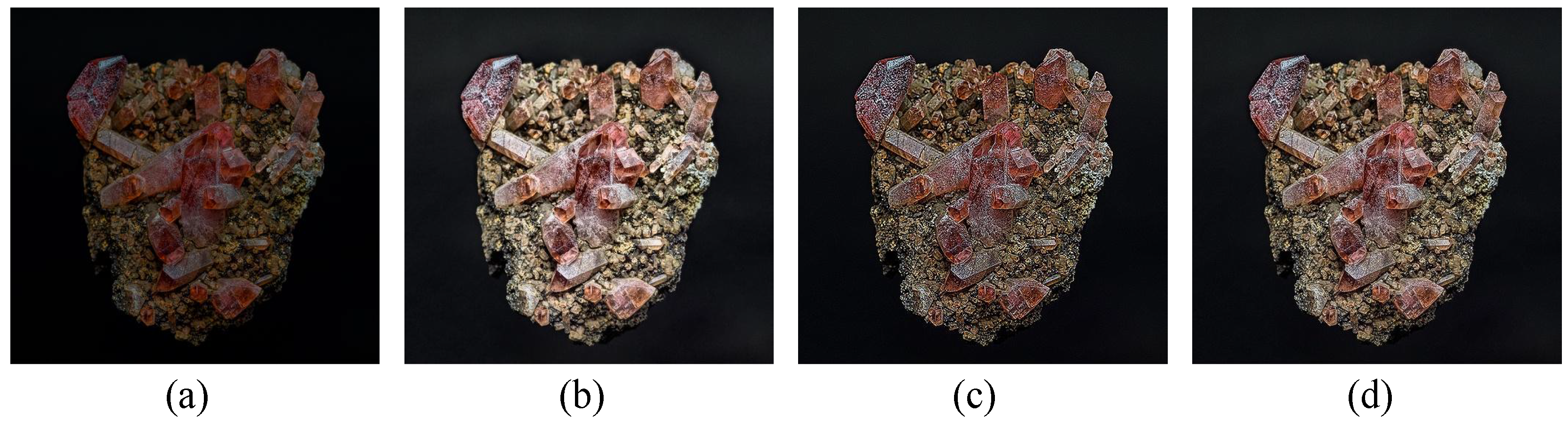
• We first propose a novel image enhancement algorithm, one which combines histogram equalization (HE) and the Laplace algorithm. In subsequent experiments, the algorithm shows powerful results.
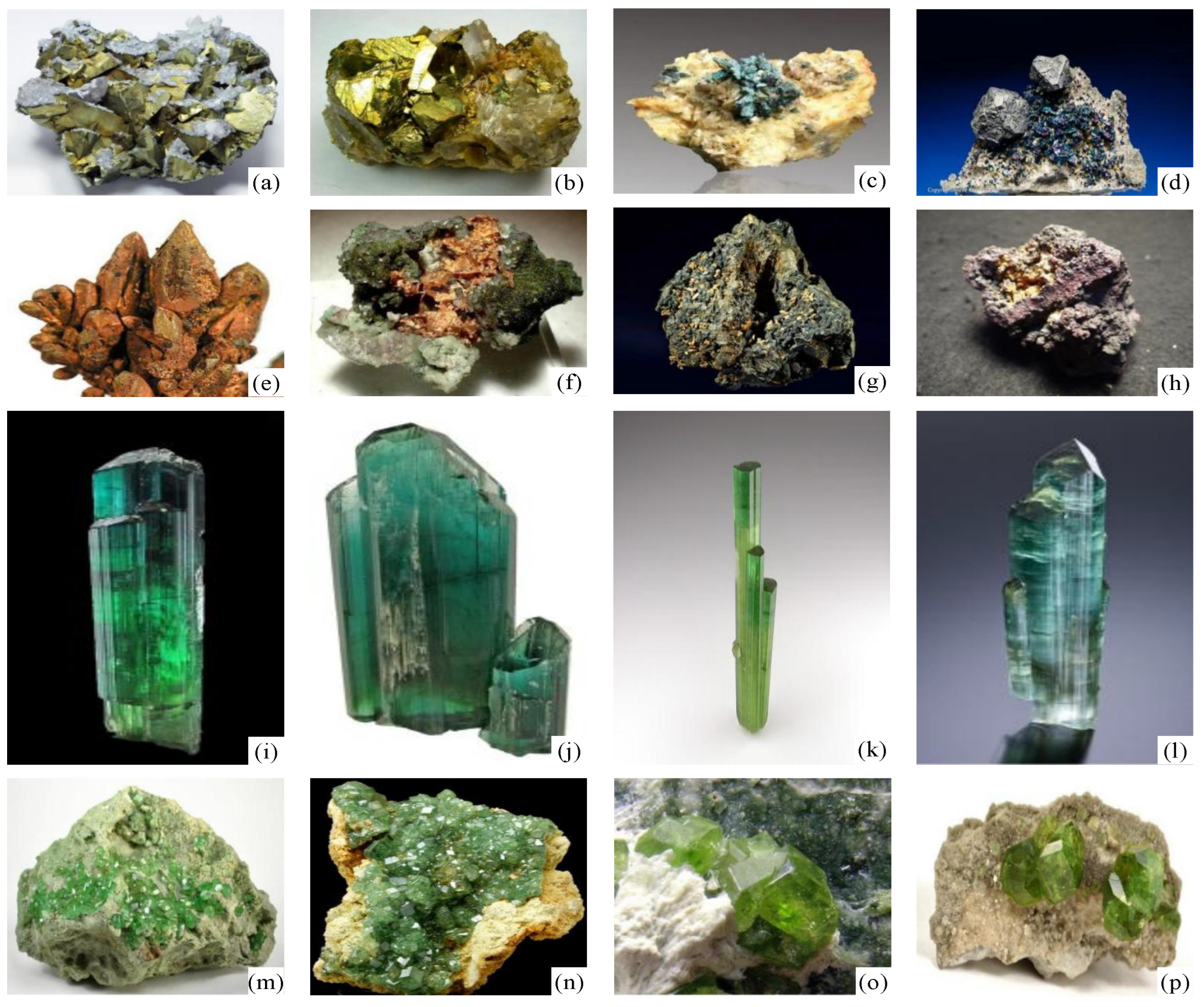
• We achieved the an efficient identification of 50 minerals, which is a significant expansion of the number of mineral species identified compared to the existing works.
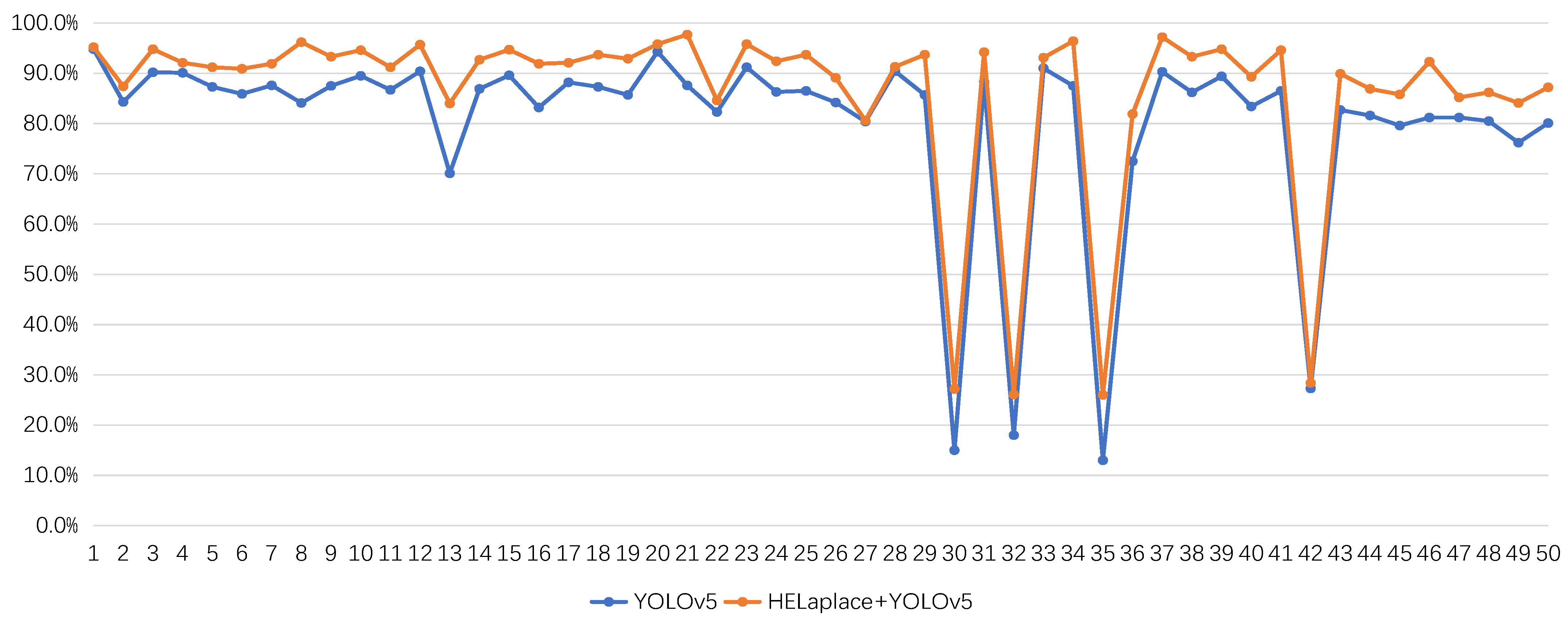
• Experiments show that our method achieves 95.6% accuracy in mineral identification, surpassing existing mineral identification methods.

The content of this paper is shown as follows. We introduce a novel image enhancement approach in Section 2, combining histogram equalization (HE) and the Laplace algorithm. In Section 3, we focus on the structure of the model we use and briefly describe the training environment and process. In Section 4, we show the results of our experiments and compare them with other methods, in addition to evaluating the model effectiveness using objective evaluation metrics. In Section 5, we conclude the article and propose future work.

2. The Proposed Method

2.1. Histogram Equalization

Histogram equalization [26] is an important method for the statistical analysis of the image grayscale distribution and is useful for images where both the background and foreground are too bright or too dark. This method enables more detail in overexposed or underexposed [27] photographs. The traditional histogram equalization method uses the cumulative distribution function of the probability of each gray level of the image as the transformation function, and according to this transformation relationship, an image with uniformly distributed gray probability density can be obtained. Its cumulative distribution function can be expressed as:

$$\begin{array}{c}\hfill s_k=T\left(r_k\right)=\sum _{j=0}^k\frac{n_j}{n}=\sum _{j=0}^k{p}_r\left(r_j\right),0⩽r_j⩽1,k=0,1,\dots ,L-1\end{array}$$

(1)

where $r_j$ is the normalized gray level before the transformation, $T\left(r_k\right)$ is the transformation function, $s_k$ is the normalized gray level after the transformation, $n_j$ is the number of pixels with the k-th gray level in the original image, n is the total number of pixels in the image, and $p_r\left(r_j\right)$ is the probability of taking the k-th gray level in the image before the transformation. However, due to its unselective data processing, it may increase the contrast of background noise and decrease the contrast of useful signals. In addition, the gray level of the transformed image is reduced and some details may be lost. Some images, such as histograms with peaks, are processed to show the unnatural over-enhancement of contrast.

2.2. Laplace Operator Image Enhancement

The Laplace operator [28] image enhancement is widely used in image processing as a second-order differential algorithm commonly used in the field of digital image processing. It causes the gray contrast to be enhanced, thus making the blurred image sharper. The essence of image blurring is that the image is subject to averaging or integration operations, so the image can be inverse operated. For example, differential operations can highlight image details and make the image sharper. Since Laplace is a differential operator, its application enhances the areas of sudden gray changes in the image and attenuates the areas of slow gray changes. Therefore, the Laplace operator can be selected to sharpen the original image to produce an image describing the abrupt grayscale changes, and then the sharpened image is produced by superimposing the Laplace image with the original image. The basic method of Laplace sharpening can be represented by the following equation.

$$\begin{array}{cc}\hfill L(x,y)& =\left\{\begin{array}{c}f(x,y)-{\nabla }^{2}f(x,y),t⩽0\hfill \\ f(x,y)+{\nabla }^{2}f(x,y),t>0\hfill \end{array}\right.\hfill \end{array}$$

(2)

where $f(x,y)$ denotes the two-dimensional image, ${\nabla }^{2}f(x,y)$ denotes its Laplace operator, and t is the neighborhood center comparison coefficient. This simple sharpening method produces the effect of a Laplace sharpening process while preserving the background information. By superimposing the original image to the processing result of the Laplace transform, we can preserve each gray value in the image so that the contrast at the gray abrupt change is enhanced. The final outcome is to bring out small details in the image while preserving the image background. However, this tends to produce a double response to image edges, which will affect the experimental results.

2.3. A New Algorithm Based on HELaplace

In order to overcome the shortcomings of the aforementioned classical histogram and Laplace algorithms, and considering the characteristics of using image fusion, this paper proposes a new algorithm for image enhancement by HELaplace. In this paper, we combine the idea of image fusion by first processing the images with histogram equalization algorithm and Laplace operator, respectively, and then fusing the processed images into a new image after weighting the average by a certain proportion. This approach demonstrates a good enhancement effect within a certain percentage range.

We convert the input image G into YCrCb (a kind of color coding method) [29] space, and then separate the YCrCb image channels and equalize the image histogram using the CLAHE [30] algorithm, which can improve the details of the image while avoiding the problem of the excessive contrast enhancement of the image. The processed channel and the unprocessed channel are combined and then converted to RGB image A. The image is then sharpened and enhanced using the 8-neighborhood Laplace operator with center 5 and image convolution, and the enhanced image is noted as B. The weighted average image fusion algorithm can be expressed as:

$$\begin{array}{c}\hfill F(i,j)=\lambda A(i,j)+(1-\lambda )B(i,j)\end{array}$$

(3)

where the input image $A(i,j)$ represents the illumination function of the image after HE algorithm processing, $B(i,j)$ represents the illumination function of the image after Laplace processing, and the output image $F(i,j)$ represents the fused image. The size of the image is 256 × 256 pixels, i and j are the coordinates of a pixel in the image, and $i,j\in [256,256]$, $A,B\in [0,255]$.

The algorithm description of HELaplace is shown in Algorithm 1. We apply the HELaplace algorithm to the same image and the result is shown in Figure 1. By comparison, we can see that the image is better after the HELaplace algorithm.

Algorithm 1 HELaplace

Input:  Original image G Output:  Synthetic image G${}_0$  1: YCrCb = COLOR_BGR2YCR_CB(G)  2: $//$ Converting RGB images to YCrCb space  3: channels = split(YCrCb)  4: $//$ Separate YCrCb image channels  5: YCrCb = merge(channels)  6: $//$ Convert YCrCb image back to RGB image  7: G${}_1$ = COLOR_YCR_CB2BGR(YCrCb)  8: kernel = np.array  9: $//$ np.array is the Laplace operator  10: G${}_2$ = filter2D(G${}_1$, cv2.CV_8UC3, kernel)  11: $//$ Convolve G with kernel  12: G${}_0$ = a*G${}_1$+b*G${}_2$  13: $//$ a,b are coefficients

3. Architecture of the Neural Network

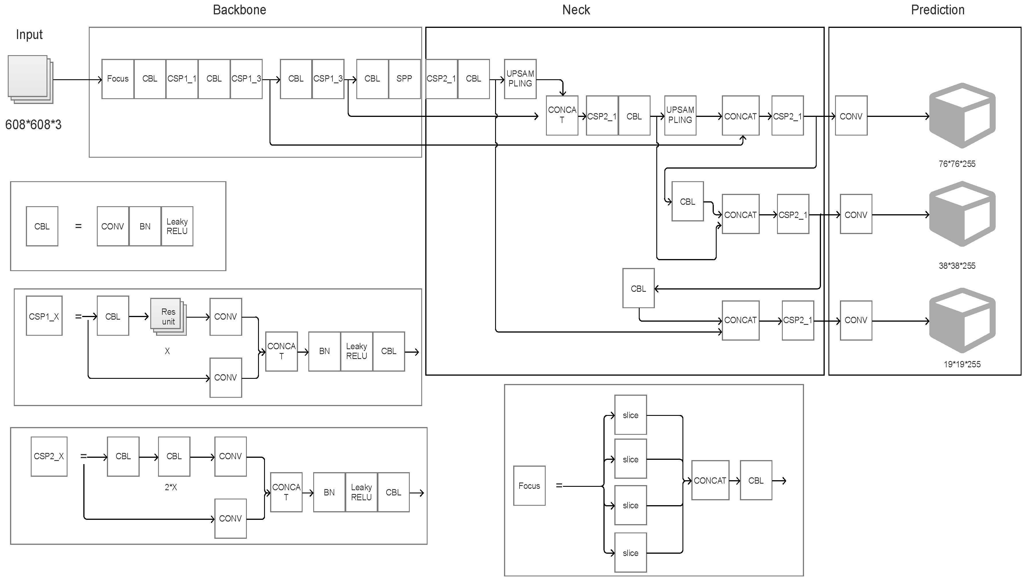
3.1. Description of Our Model

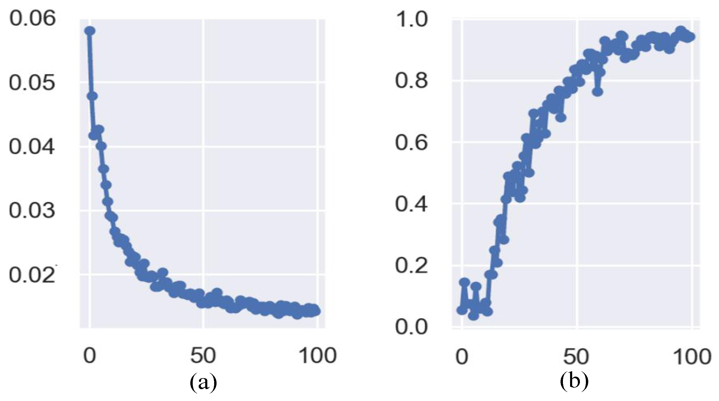
The main procedure of the experiment is shown in Figure 2. First, we collect data on a variety of minerals. Then, we label all the data and split the dataset into a training set and a test set. HELaplace processing is performed on the data from the test set and training set. Then, the obtained training set is used to train in a convolutional neural network through the YOLOv5 model. Finally, the classification to which each mineral picture in the test set belongs is calculated and the accuracy rate is recorded.

Specifically, Figure 3 illustrates the specific structure of the YOLOv5 network. It consists of four parts: input, backbone, neck, and prediction. The input side uses Mosaic data enhancement [23] and adaptive anchor frame calculation. The backbone part uses the focus structure and the cross-stage-partial-connections (CSP) structure. The neck part uses a feature pyramid network (FPN) + pixel aggregation network (PAN)) structure. The prediction part uses non-maximal suppression (NMS) to filter the targets, so it has high accuracy. As a new type of deep neural network (DNN), unlike traditional algorithms that require strict image pixel size, YOLOv5’s adaptive image scaling has no requirement in terms of image size. We also modified the YOLOv5 code in the letterbox function of datasets.py to add a minimum of black borders to the adaption of the original image, reducing information redundancy and therefore greatly improving the processing speed. The CSP structure of YOLOv5s is to divide the original input into two branches and perform separate convolution operations to halve the number of channels. One branch performs the Bottleneck * N operation, then concats two branches. This allows the input and output of BottlenneckCSP to be the same size, which enables the model to learn more features. The neck of YOLOv5 has the same FPN+PAN structure as in YOLOv4. However, the convolution operation used in the neck of YOLOv4 is regular. In contrast, the CSP2 structure inspired by the CSPNet [31] design is used in the neck structure of YOLOv5 to enhance the network feature fusion and improve the identification accuracy.

3.2. Model Training

In this paper, the deep learning integrated development environment is Pycharm. Test environment: NVIDIA GTX 1060, 8G memory, Intel Core(TM) i7-8750H CPU, and Python 3.8 as the compiler language. The parameters we used for model training are shown in

Table 2. Parameters used for model training.

Parameters	Configuration
Pre-training weight	YOLOV5S.PT
Epochs	100
Sample size	183,380
Conf-thres	0.05
Iou-thres	0.45
Img-size	640
Batch-size	10

. Parameters not listed in the table are used as default values.

In our experiments, we use the GLOU function [32] as our loss function. Its smaller value indicates more accurate results. The expression of its function is

$$\begin{array}{cc}\hfill {\mathrm{Glou}}_{\mathrm{loss}}& =-\frac{1}{{\sum }_{p}1}\sum _p\left(1-{lou}_p\right)\hfill \end{array}$$

(4)

where p denotes the predicted positive example index and lou${}_p$ is the intersection ratio of the predicted positive example frame p to the corresponding true frame.

We recorded the changes in loss function GLOU values during the training process and tested the accuracy of the model on the validation set after each iteration of the training set was completed. The change in GLOU loss during the training process is shown in Figure 4. It can be seen that the model converges effectively, and the GLOU loss has reached a low level after 50 epochs. According to the figure, the model achieves the best accuracy on the validation set after the 90th iteration, and the accuracy decreases after continuing the training, probably due to some overfitting.

4. Test Result and Discussion

To test the accuracy of our method, we selected 13,911 images from a collection of 220,057 images for testing our neural network model. After inputting one of the images into the neural network, the mineral category with the highest probability is given. We evaluate the performance of our method in terms of accuracy, and also compare it with other methods and give results.

4.1. Data

The training of mineral identification using YOLOv5 requires a large amount of data during validation and testing. The more data available for training, the more generalizable and robust the model will be, and the higher the accuracy will be. To obtain a large amount of specialized image data for a wide range of minerals, we chose to use image data from Mindat [33]. Mindat is a community-led global mineral and provenance database website and the world’s largest database of mineral information. In this paper, one mineral is selected as a training representative in the database according to the mineral category criteria [33] in each mineral major category to obtain adequate category coverage. To further extend the mineral coverage categories, we expanded 26 minerals from those covered by work [16]. Therefore, the images of a total of 50 minerals were collected as experimental samples. The names of relevant minerals and the number of samples are shown in

Table 3. Names of the minerals and the number of samples.

#No.	Mineral	Number of Samples	#No.	Mineral	Number of Samples
1 2 3 4 5 6 7 8 9 10 11 12 13 14 15 16 17 18 19 20 21 22 23 24 25	Adularia Aegirine Agate Albite Almandine Amber Anglesite Azurite Beryl Biotite Boracite Cassiterite Chalcopyrite Cinnabar Copper Demantoid Diopside Elbaite Epidote Fluorite Galena Goethite Gold Gypsum Halite	738 909 3636 1882 2124 294 1981 8320 9836 1437 240 3321 3296 1618 5504 785 1649 5683 3915 28,147 6661 4063 4796 2439 821	26 27 28 29 30 31 32 33 34 35 36 37 38 39 40 41 42 43 44 45 46 47 48 49 50	Hematite Magnetite Malachite Marcasite Moissanite Niccolite Nitratine Opal Orpiment Ozocerite Pyrite Quartz Rhodochrosite Ruby Sapphire Schorl Selenium Sphalerite Stibnite Sulphur Topaz Torbernite Turquoise Whewellite Wulfenite	6086 2615 7919 1748 10 245 10 3283 754 23 13,042 46,398 4510 872 1056 2200 106 6412 2548 1843 3926 1170 988 94 8104
Total			220,057

. Among them, the small numbers of samples of certain minerals are due to their rarity, which makes it difficult to obtain a large number of samples. It is worth noting that all samples of minerals in this paper are labeled according to the classification criteria of Mindat.

Since some of the images directly obtained from the website were taken under a microscope or after processing, this may have some influence on the experimental results. Therefore, we artificially removed the images that did not meet the requirements in the dataset during the collection process. We uniformly mixed each of the obtained mineral images in the ratio of 10:1:1 and separated them into a training set, a validation set, and a test set. An example of the mineral images is shown in Figure 5.

4.2. Test Result

We used the YOLOv5 neural network and HELaplace+YOLOv5 neural network to test images with too little light and too much light, respectively, and the average accuracy obtained is shown in

Table 4. Comparison of the accuracy of different methods.

Method	Accuracy
YOLOv5 HE + YOLOv5 Laplace + YOLOv5 HELaplace + YOLOv5	85.31% 87.14% 86.82% 95.63%

. The test results show that the combination of the HELaplace and YOLOv5 algorithms can greatly improve the identification accuracy. Figure 6 shows the accuracy of mineral identification for all 50 categories. As we can see, except for specific minerals, all of our minerals are identified with an accuracy of more than 80%. Among them, four minerals possess relatively low accuracy due to the a small number of training samples, which include Moissanite, Nitratine, Ozocerite and Selenium. Using HELaplace in combination with YOLOv5, the accuracy of all mineral species was improved compared to the results without using HELapace, especially the identification accuracy of minerals (Azurite, Chalcopyrite, Galena, Topaz) which was improved by 10%. The main reason is that the images taken in insufficiently or excessively bright light will have chromatic aberrations due to the light, many minerals have similar shapes and textures, and the resulting chromatic aberrations make it difficult for the model to correctly identify them based on the images. After applying HELaplace, the minerals (Adularia, Magnetite, and Malachite) do not significantly improve the accuracy, which is due to the fact that these minerals themselves are too dark and less influenced by light. It can be seen from Table 4 and Figure 6 that combining HELaplace with YOLOv5 can improve the identification accuracy of most minerals.

4.3. Comparison with Other Methods

Table 5. Comparison of deep learning-based and image-based mineral identification works.

Studies	Accuracy (%)	Number of Identified Minerals	Image Type
[10]	89	5	Microscopic
[11]	95	2	Microscopic
[12]	90	9	Microscopic
[13]	90.9	4	Microscopic
[14]	90	4	Microscopic
[15]	95.4	23	Microscopic
[34]	\	23	CT
[35]	94.2	5	Raman spectra
[16]	90.6	36	Photo and hardness
[17]	86	16	Photo
[18]	90	7	Photo
Our method	95.6	50	Photo

demonstrates the number and accuracy of identified minerals for existing mineral detection methods. In contrast to the dual-energy CT chemometric calibration method [34], our work does not require the use of instruments for the medical X-ray tomography of minerals. Compared to the method using polarized light microscopy to obtain images [10], which can only identify five minerals, our method can identify 50 species with similar accuracy. Similarly, compared to the work of Julio et al. [11] which could only distinguish between resin and quartz, we were able to differentiate more minerals and maintain a similar accuracy. Furthermore, in contrast, we do not need special instruments to obtain the picture data under the polarized light microscope, we only need to take pictures of the minerals to perform the identification. In contrast to the work of Zeng et al. [16] who used Mohs hardness and images to identify minerals, our work does not require the use of instruments to obtain Mohs hardness. It is worth noting that the aforementioned work on identification using mineral images was experimentally measured using images taken under normal lighting, and when experiments were conducted using images taken under excessively dark or excessively bright conditions, the accuracy rate would be reduced to varying degrees.

4.4. Objective Evaluation Indicators

Since it is difficult to obtain the normal illumination image corresponding to the image under abnormal illumination, for the image quality after enhancement, natural image quality evaluator (NIQE) [36] was used in this paper. NIQE is a non-reference image quality index often used to measure the quality of the image, a smaller NIQE indicating a better the quality of the measured picture. In addition, we used the lightness-order-error (LOE) [37] to evaluate the contrast of the enhanced image with the original illuminated image. LOE reflects the natural retention of the image, and a smaller value indicates that the image has a better order of luminance and therefore looks more natural.

Table 6. Result of LOE and NIQE.

Index	HE	Laplace	HELaplace
LOE	222.6444	156.2836	150.7435
NIQE	25.3780	41.7903	25.2050

shows the objective evaluation data of the corresponding methods in Figure 1. From the data in the table, we can see that the LOE of our algorithm is lower than that of the Laplace algorithm, and it is the lowest among all algorithms, indicating that we have the best result in maintaining the naturalness of the image. Furthermore, the NIQE value of the algorithm in this paper is the lowest among all algorithms, which indicates that the method in this paper does not produce much detail, thus blurring and color distortion to the original image.

5. Conclusions and Future Work

In this paper, we propose a deep learning mineral identification method based on luminance equalization. Compared with traditional mineral identification methods, we reduce the reliance on the researcher’s experience and instruments. Compared with traditional mineral identification algorithms, we reduce the influence of illumination intensity on mineral identification and greatly improve the accuracy rate. In the deep learning recognition part, we used YOLOv5 to further improve the identification accuracy. During model selection, we used the optimized YOLOv5 to further improve the identification accuracy. In the future, more features will be introduced, such as combining the density and transparency of minerals with photos to further improve the accuracy of mineral identification. However, the identification method mentioned in this paper has some limitations: when the input picture is a mineral other than fifty minerals, the closest one among fifty minerals will be given. In the future, we will collect more mineral data to address this issue.

References

1. Lu, Y.; Yang, K.; Xiu, L. Identification of hydrocarbon and clay minerals based on near-infrared spectroscopy and its geological significance. Geol. Bull. China 2017, 36, 1884–1891. [Google Scholar]
2. Wang, R.-S.; Yang, S.-M.; Yan, B.K. A review of mineral spectral identification methods and models with imaging spectrometer. Remote Sens. Land Resour. 2007, 19, 1–9. [Google Scholar]
3. Porwal, A.; Carranza, E.; Hale, M. Artificial neural networks for mineral-potential mapping: A case study from Aravalli Province, Western India. Nat. Resour. Res. 2003, 12, 155–171. [Google Scholar] [CrossRef]
4. Li, S.; Chen, J.; Liu, C.; Wang, Y. Mineral prospectivity prediction via convolutional neural networks based on geological big data. J. Earth Sci. 2021, 32, 327–347. [Google Scholar] [CrossRef]
5. Lou, W.; Zhang, D.; Bayless, C.R. Review of Mineral Recognition and Its Future. Appl. Geochem. 2020, 122, 104727. [Google Scholar] [CrossRef]
6. Ruisanchez, I.; Potokar, P.; Zupan, J.; Smolej, V. Classification of Energy Dispersion X-ray Spectra of Mineralogical Samples by Artificial Neural Networks. J. Chem. Inf. Model. 1996, 36, 214–220. [Google Scholar] [CrossRef]
7. Tsuji, T.; Yamaguchi, H.; Ishii, T.; Matsuoka, T. Mineral classification from quantitative X-ray maps using neural network: Application to volcanic rocks. Island Arc 2010, 19, 105–119. [Google Scholar] [CrossRef]
8. El Haddad, J.; de Lima Filho, E.S.; Vanier, F.; Harhira, A.; Padioleau, C.; Sabsabi, M.; Wilkie, G.; Blouin, A. Multiphase mineral identification and quantification by laser-induced breakdown spectroscopy. Miner. Eng. 2019, 134, 281–290. [Google Scholar] [CrossRef]
9. Liu, J.; Osadchy, M.; Ashton, L.; Foster, M.; Solomon, C.J.; Gibson, S.J. Deep convolutional neural networks for raman spectrum recognition: A unified solution. Analyst 2017, 142, 4067–4074. [Google Scholar] [CrossRef] [Green Version]
10. Guo, Y.; Zhou, Z.; Lin, H.; Liu, X.; Chen, D.; Zhu, J.; Wu, J. The mineral intelligence identification method based on deep learning algorithms. Earth Sci. Front. 2020, 27, 39–47. [Google Scholar]
11. Álvarez Iglesias, J.C.; Santos, R.B.M.; Paciornik, S. Deep learning discrimination of quartz and resin in optical microscopy images of minerals. Miner. Eng. 2019, 138, 79–85. [Google Scholar] [CrossRef]
12. Maitre, J.; Bouchard, K.; Bédard, L.P. Mineral grains recognition using computer vision and machine learning. Comput. Geosci. 2019, 130, 84–93. [Google Scholar] [CrossRef]
13. Zhang, Y.; Li, M.; Han, S.; Ren, Q.; Shi, J. Intelligent Identification for Rock-Mineral Microscopic Images Using Ensemble Machine Learning Algorithms. Sensors 2019, 19, 3914. [Google Scholar] [CrossRef] [Green Version]
14. Xu, S.; Zhou, Y. Artificial intelligence identification of ore minerals under microscope based on deep learning algorithm. Acta Petrol. Sin. 2018, 34, 3244–3252. [Google Scholar]
15. Izadi, H.; Sadri, J.; Mehran, N.A. Intelligent mineral identification using clustering and artificial neural networks techniques. In Proceedings of the Conference on Pattern Recognition and Image Analysis, Birjand, Iran, 6–8 March 2013; pp. 1–5. [Google Scholar]
16. Zeng, X.; Xiao, Y.; Ji, X.; Wang, G. Mineral Identification Based On Deep Learning That Combines Image And Mohs Hardness. Minerals 2021, 11, 506. [Google Scholar] [CrossRef]
17. Peng, W.; Bai, L.; Shang, S.; Tang, X.; Zhang, Z. Common mineral intelligent recognition based on improved InceptionV3. Geol. Bull. China 2019, 38, 2059–2066. [Google Scholar]
18. Ramil, A.; López, A.; Pozo-Antonio, J.; Rivas, T. A computer vision system for identification of granite-forming minerals based on RGB data and artificial neural networks. Measurement 2018, 117, 90–95. [Google Scholar] [CrossRef]
19. Li, Z.; Jia, Z.; Yang, J.; Kasabov, N. A method to improve the accuracy of SAR image change detection by using an image enhancement method. ISPRS J. Photogramm. Remote Sens. 2020, 163, 137–151. [Google Scholar] [CrossRef]
20. Xiao, Y.; Jiang, A.; Ye, J.; Wang, M.W. Making of Night Vision: Object Detection Under Low-Illumination. IEEE Access 2020, 8, 123075–123086. [Google Scholar] [CrossRef]
21. Xiong, J.; Zou, X.; Wang, H.; Peng, H.; Zhu, M.; Lin, G. Recognition of ripe litchi in different illumination conditions based on Retinex image enhancement. Trans. Chin. Soc. Agric. Eng. 2013, 29, 170–178. [Google Scholar]
22. Tan, M.; Pang, R.; Le, Q.V. Efficientdet: Scalable and efficient object detection. In Proceedings of the IEEE/CVF Conference on Computer Vision and Pattern Recognition, Seattle, WA, USA, 13–19 June 2020; pp. 10781–10790. [Google Scholar]
23. Bochkovskiy, A.; Wang, C.Y.; Liao, H.Y.M. Yolov4: Optimal speed and accuracy of object detection. arXiv 2020, arXiv:2004.10934. [Google Scholar]
24. Xu, Q.; Zhu, Z.; Ge, H.; Zhang, Z.; Zang, X. Effective Face Detector Based on YOLOv5 and Superresolution Reconstruction. Comput. Math. Methods Med. 2021, 2021, 7748350. [Google Scholar] [CrossRef] [PubMed]
25. Li, S.; Li, Y.; Li, Y.; Li, M.; Xu, X. YOLO-FIRI: Improved YOLOv5 for Infrared Image Object Detection. IEEE Access 2021, 9, 141861–141875. [Google Scholar] [CrossRef]
26. Pizer, M.S.; Amburn, P.E.; Austin, D.J.; Cromartie, R.; Geselowitz, A.; Greer, T.; Romeny, T.H.B.; Zimmerman, B.J. Adaptive histogram equalization and its variations. Comput. Vis. Graph. Image Process. 1987, 39, 355–368. [Google Scholar] [CrossRef]
27. Jebadass, J.R.; Balasubramaniam, P. Low contrast enhancement technique for color images using interval-valued intuitionistic fuzzy sets with contrast limited adaptive histogram equalization. Soft Comput. 2022, 26, 4949–4960. [Google Scholar] [CrossRef]
28. Van Vliet, L.J.; Young, I.T.; Beckers, G.L. A nonlinear laplace operator as edge detector in noisy images. Comput. Vis. Graph. Image Process. 1989, 45, 167–195. [Google Scholar] [CrossRef] [Green Version]
29. Szedo, G. Color-Space Converter: RGB to YCrCb; Xilinx Corp.: San Jose, CA, USA, 2006. [Google Scholar]
30. Reza, A.M. Realization of the contrast limited adaptive histogram equalization (CLAHE) for real-time image enhancement. J. VLSI Signal Process. Syst. Signal Image Video Technol. 2004, 38, 35–44. [Google Scholar] [CrossRef]
31. Wang, C.Y.; Liao, H.Y.M.; Wu, Y.H.; Chen, P.Y.; Hsieh, J.W.; Yeh, I.H. CSPNet: A New Backbone that can Enhance Learning Capability of CNN. In Proceedings of the IEEE/CVF Conference on Computer Vision and Pattern Recognition Workshops, Long Beach, CA, USA, 16–17 June 2019. [Google Scholar]
32. Rezatofighi, H.; Tsoi, N.; Gwak, J.; Sadeghian, A.; Reid, I.; Savarese, S. Generalized intersection over union: A metric and a loss for bounding box regression. In Proceedings of the IEEE/CVF Conference on Computer Vision and Pattern Recognition, Long Beach, CA, USA, 16–17 June 2019; pp. 658–666. [Google Scholar]
33. A Mineral Database. Available online: https://www.mindat.org/ (accessed on 7 June 2022).
34. Martini, M.; Francus, P.; Trotta, D.S.L.; Despres, P. Identification of Common Minerals Using Stoichiometric Calibration Method for Dual-Energy CT. Geochem. Geophys. Geosyst. 2021, 22, e2021GC009885. [Google Scholar] [CrossRef]
35. Zhang, X.; Yu, M.; Zhu, L.; He, Y.; Sun, G. Raman mineral recognition method based on all-optical diffraction deep neural network. Infrared Laser Eng. 2020, 49, 20200221-1–20200221-8. [Google Scholar]
36. Mittal, A.; Soundararajan, R.; Bovik, A.C. Making a “completely blind” image quality analyzer. IEEE Signal Process. Lett. 2012, 20, 209–212. [Google Scholar] [CrossRef]
37. Wang, S.; Zheng, J.; Hu, H.M.; Li, B. Naturalness preserved enhancement algorithm for non-uniform illumination images. IEEE Trans. Image Process. 2013, 22, 3538–3548. [Google Scholar] [CrossRef] [PubMed]
Figure 1. (a) Original image; (b) image processed by HE; (c) image processed by Laplace; and (d) image processed by HELaplace.
Applsci 12 07055 g001
Figure 2. The structure of our model.
Applsci 12 07055 g002
Figure 3. The main model of YOLOv5 network.
Applsci 12 07055 g003
Figure 4. Change in (a) loss value and (b) precision value.
Applsci 12 07055 g004
Figure 5. Examples of cropped images ((ad) chalcopyrite; (eh) copper; (il) elbaite; and (mp) demantoid). The original images are from Mindat.
Applsci 12 07055 g005
Figure 6. Accuracy comparison of specific mineral species.
Applsci 12 07055 g006