An Enhanced Proximal Policy Optimization-Based Reinforcement Learning Method with Random Forest for Hyperparameter Optimization

Abstract

For most machine learning and deep learning models, the selection of hyperparameters has a significant impact on the performance of the model. Therefore, deep learning and data analysis experts have to spend a lot of time on hyperparameter tuning when building a model for accomplishing a task. Although there are many algorithms used to solve hyperparameter optimization (HPO), these methods require the results of the actual trials at each epoch to help perform the search. To reduce the number of trials, model-based reinforcement learning adopts multilayer perceptron (MLP) to capture the relationship between hyperparameter settings and model performance. However, MLP needs to be carefully designed because there is a risk of overfitting. Thus, we propose a random forest-enhanced proximal policy optimization (RFEPPO) reinforcement learning algorithm to solve the HPO problem. In addition, reinforcement learning as a solution to HPO will encounter the sparse reward problem, eventually leading to slow convergence. To address this problem, we employ the intrinsic reward, which introduces the prediction error as the reward signal. Experiments carried on nine tabular datasets and two image classification datasets demonstrate the effectiveness of our model.

1. Introduction

Machine learning (ML) models have exploded in complexity in recent years at the expense of high computational costs [1]. ML is actually the calculation process of learning data through a certain algorithm. Parameters that can be updated during the training process are called model parameters. There is another kind of parameter, hyperparameter, which should be defined before training and cannot be learned from the normal training process. For instance, the kernel, regularization parameter, and kernel coefficient of a support vector machine (SVM), and the hidden state size and learning rate of a deep learning (DL) model are all hyperparameters. The process of finding the optimal hyperparameters is inevitable since hyperparameters have a remarkable effect on the performance in terms of time or accuracy of the model. In many cases, engineers rely on the trial-and-error method to manually tune hyperparameters. Even experienced engineers will try multiple times in a certain range to find the optimal combination of hyperparameters, not to mention that for non-experts in ML and DL, finding the best hyperparameters is time consuming and difficult.

To solve this issue, automated ML (AutoML) has been proposed, which can build ML pipelines on a limited computational budget automatically, without human interference. The overall process of AutoML consists of four phases: data preparation, feature engineering, model generation, and model evaluation [2]. The optimization method is a part of model generation, which can be further divided into architecture optimization (AO) and hyperparameter optimization (HPO). Thornton et al. [3] defined the automatic selection of learning algorithms and the setting of hyperparameters to optimize empirical performance as a combined algorithm selection and hyperparameter optimization (CASH) problem. In this work, we focus on the HPO task.

In practice, HPO is confronted with many challenges, which make it a difficult problem. First, the hyperparameter tuning of ML models is generally considered a black-box optimization problem, that is, we can only observe the inputs and outputs of the model during the tuning process. We usually cannot obtain the gradient of the cost function with respect to the hyperparameters. Second, when facing large models, large datasets, the target model needs to be trained with selected hyperparameters to obtain the loss value, so the process of evaluation is very expensive. Finally, the configuration space is very complex and high dimensional. For a given algorithm, there are multiple hyperparameters correspondingly, and each hyperparameter has its own range of values.

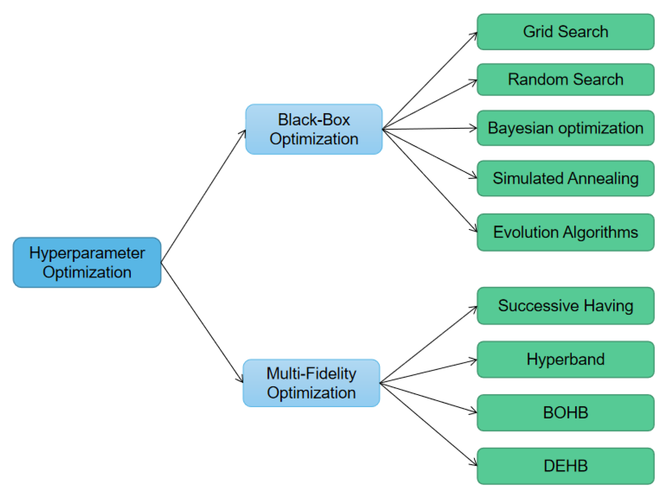
Recently, many methods are used to solve HPO problem, and several libraries have implemented these methods to allow researchers to conveniently work with them, such as Hyperopt (https://github.com/hyperopt/hyperopt, accessed on 16 May 2022), HpBandSter (https://github.com/automl/HpBandSter, accessed on 16 May 2022), SMAC (https://github.com/automl/SMAC3, accessed on 16 May 2022), Sherpa [4], etc. The methods shown in Figure 1 are mainly classified into two categories:

• Black-box optimization, e.g., grid search (GS) [5], random search (RS) [6], Bayesian optimization (BO) [7,8], simulated annealing (SA) [9], and evolution algorithm (EA) [10].
• Multi-fidelity optimization, e.g., successive having (SH) [11], hyperband [1], Bayesian optimization hyperband (BOHB) [12], and differential evolution hyperband (DEHB) [13].

GS is very simple and can be executed in parallel; however, the number of trials increases exponentially with the number of hyperparameters. Compared to GS, RS is more efficient, but it does not guarantee finding the global optimum in the limit, whereas GS never will. A typical BO method is to adopt a Gaussian process (GP) as the surrogate model; however, GP is cubically related to the number of data sizes. Hyperband dynamically allocates resources to each set of configurations and uses SH to stop underperforming configurations. However, it randomly samples new configurations at each step. In order to learn the previously sampled configurations, BOHB combines BO with hyperband, and DEHB combines the evolutionary optimization method of differential evolution (DE [14]) with hyperband. However, these hyperband-based methods tend to choose the hyperparameter settings that enable the model to converge quickly in the early stages of training. Wu et al. [15] used the reinforcement learning (RL) method and treated HPO as a sequential decision process. In addition, to speed up training, they used MLP as a surrogate model to predict accuracy and dynamically train the agent with true accuracy and predicted accuracy. This approach reduces the number of trials and does not tend to choose a hyperparameter setting that converges quickly in the early stages of training. However, due to the sequential selection of hyperparameters, the reward is obtained only when the last hyperparameter is selected, and the rewards of previous steps are all 0, which causes the problem of sparse reward. Moreover, the MLP model needs to be carefully designed and requires a large sample size to prevent overfitting. Inspired by [15], we adopt random forest (RF) as a surrogate model and use part of the real rewards and part of the predicted rewards from the surrogate model when updating the agent. Moreover, in order to solve the problem of sparse reward, we add the curiosity to provide intrinsic reward.

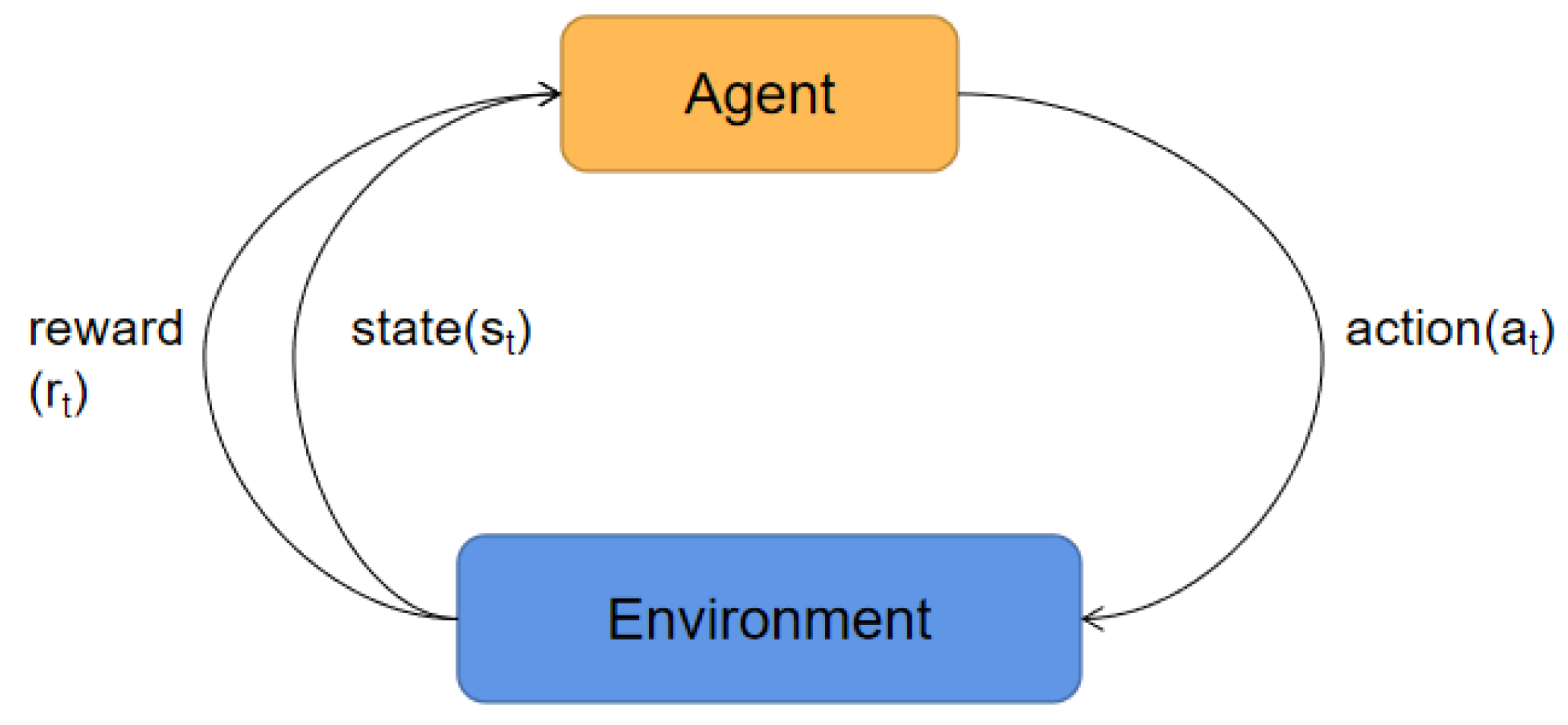
The basic process of RL-based HPO is shown in Figure 2. The agent observes state $s_t$ in the environment at time step t and then executes action $a_t$ according to the policy. Consequently, the environment returns a reward $r_t$ to the agent, and the state is transferred from $s_t$ to $s_{t+1}$. For the environment, state, action and reward of this paper, we introduce them in detail in Section 3.

In this work, we use the proposed method to optimize the hyperparameters of extreme gradient boosting (XGBoost) [16] on nine tabular datasets and convolutional neural network (CNN) on two image datasets. The main contributions of this paper are as follows:

• We use the RF algorithm as a surrogate model which can predict rewards and then reduce the consumption of resources.
• For the sparse reward problem of HPO, we use curiosity to provide an intrinsic reward that speeds up the convergence and finds better hyperparameter configuration faster.
• We use the proposed method to tune the hyperparameters of the XGBoost on nine tabular datasets and CNN models on two image datasets. The experimental results show that our method has higher accuracy and faster convergence compared to other optimization algorithms.

The remainder of this paper is organized into four sections. Section 2 introduces the hyperparameter optimization methods and the optimization objective of RL. In Section 3, we describe our proposed method. Section 4 displays and discusses the experiment results. Finally, we draw conclusions in Section 5.

2. Related Work

2.1. Hyperparameter Optimization

HPO is a task to find the optimal/suboptimal hyperparameters in ML/DL models by using certain algorithms. HPO generally consists of three components: the first is the objective function, i.e., the goal that the algorithm needs to minimize or maximize; the second is the search range, which needs to determine candidates for discrete spaces and upper and lower bounds for continuous spaces; and the third is the parameters of the algorithm itself, such as the selection of acquisition functions. The definition of HPO is as follows: Let $\mathcal{A}$ denote a ML or DL algorithm with n hyperparameters; ${\mathcal{A}}_{\lambda }$ is the algorithm $\mathcal{A}$ with hyperparameter $\lambda$; ${\Lambda }_n$ is the search space of the n-th hyperparameter; and $\Lambda$ denotes all hyperparameter search spaces. Therefore, given a data set $\mathcal{D}$, the purpose of HPO is to find

$${\lambda }^{*}=\underset{\lambda \in \Lambda }{argmin}{\mathbb{E}}_{(D_{train},D_{valid})\sim \mathcal{D}}\mathcal{L}({\mathcal{A}}_{\lambda },D_{train},D_{valid})$$

(1)

where $\mathcal{L}({\mathcal{A}}_{\lambda },D_{train},D_{valid})$ denotes the loss value of model $\mathcal{A}$ with hyperparameter setting $\lambda$ on validation data set $D_{valid}$ that is trained on training set $D_{train}$.

Some popular hyperparameter tuning algorithms have been proposed in recent years and widely used in different fields.

Grid search and random search: GS defines the search space as a regular grid and evaluates every position in the grid. With a large search range and a small step size, GS has a high probability of discovering the global optimum. However, this method is very computationally intensive and time consuming, especially when the number of hyperparameters to be tuned is relatively large. The idea of RS is similar to GS, but it is generally faster than GS. Instead of testing all values in the grid, RS randomly selects sample points within the search space. RS assumes that if the set of sample points is sufficiently large, then the global optimum or its approximation can also be found with a high probability through random sampling.

Bayesian optimization: BO is an effective optimization method and generally used for optimizing expensive black-box functions [17]. BO finds the value that minimizes the objective function based on the historical evaluation results by building a surrogate function (probabilistic model). Several surrogate models commonly used in BO are Gaussian process (GP), tree-structured Parzen estimator (TPE) [5], and RF. The Bayesian based approach differs from grid or random search in that it saves a lot of useless work by referring to previous evaluations when trying the next set of hyperparameters.

Evolutionary algorithm-based optimization: The idea of the EA method comes from the concept of biology. Since natural evolution is a dynamic process occurring in a changing environment, it is applicable to the HPO task, which is also a dynamic process. The covariance matrix adaptation evolution strategy (CMA-ES) [18] is one of the most well-known EA methods. EA can also be used to optimize the neural structure and hyperparameters of deep learning models [19].

Bandit-based optimization: It is very expensive to verify the performance of different hyperparameters when the data set is very large or the model is very complex. Common techniques to address this problem include using subsets of the data set, feature dimensionality reduction, reducing training steps, etc. However, the multi-fidelity approach converts this manual heuristic into a formal algorithm that uses an approximation of the real loss function for optimization [20]. Typical bandit-based methods are hyperband and successive halving. The BOHB proposed in [12] utilizes hyperband to decide how many sets of hyperparameters to use at a time and how much budget to allocate to each set of hyperparameters. In addition, BOHB uses BO to select hyperparameters instead of random selection as hyperband does [21]. The DEHB proposed in [13] combines DE and HB, which maintains a sub-population for each budget level and uses the size of the sub-population as the maximum number of hyperparameter configurations for the corresponding budget level.

2.2. Reinforcement Learning

RL is an area of ML that aims to allow agents to take actions in an environment in order to maximize their expected benefits. The RL problems are often modeled by an MDP, which was first proposed by Bellman [22]. Watkins first attempted with MDP modeling in RL [23]. MDP is usually defined as a tuple $<S,A,P,\gamma ,R>$, where S denotes the state set with $s\in S$ and $s_i$ denotes the state at step i; A denotes a set of actions with $a\in A$ and $a_i$ denotes the action at step i; P is the probability of transition from one state of a system into another state; R is the reward function; and $\gamma$ is the discount factor. The purpose of RL is to allow agents to learn an optimal policy or near-optimal policy that maximizes the expectation of the discount reward sum. The policy can be expressed by

$$\pi (a,s)=Pr(a_t=a|s_t=s)$$

(2)

where $\pi (a,s)$ represents the probability of choosing action a in state s at step t.

RL can be classified into two types: value-based (e.g., Q Learning [24]) and policy-based (e.g., TRPO [25]). Q Learning constructs a Q table to store Q values and updates it with a weighted sum of the expected values of over all future steps from this state after the execution of the action. It is clear that traditional Q Learning cannot handle tasks with too many states and optional actions. Deep Q Network (DQN) [26] combines DL models with RL to successfully learn policies from high-dimensional inputs directly. These value-based RL methods are relatively well used in many fields, but they have several limitations. For example, they do not have enough ability to handle continuous actions and cannot solve the stochastic policy problem. To solve these problems, policy-based methods with an estimated representation of the policy are introduced. However, selecting the appropriate step size for the policy-based methods is challenging because it is very sensitive to the step size. TRPO is able to find the right step size at each step and reliable performance, but it is relatively complicated. The proximal policy optimization (PPO) proposed in [27] takes some benefits of TRPO and makes the implementation simpler and more general by using first-order optimization, and has better sample complexity. Therefore, in this paper, we choose to enhance the PPO algorithm and apply it on HPO task.

RL was previously used for neural architecture search (NAS). Zoph et al. [28] first used the policy gradient algorithm to train an agent; the agent samples architecture from the search space and receives reward from the environment, which refers to the neural network training procedure. More recently, RL was also used for HPO. Jomaa et al. [29] used Q Learning to tune hyperparameters on 50 classification datasets. Ref. [30] adopted context-based meta-RL to help the agent to quickly identify task by learning from past experience. However, the problem of sparse reward was ignored in all these studies.

3. Methodology

In this section, we first transform the HPO task into an MDP task for RL. Second, we introduce the agent and training algorithm of RL that we use in this task. Finally, we describe our enhanced part.

3.1. MDP Formulation

MDP is a mathematical model for the sequential decision problem. It is often used to model the stochastic policies and rewards achievable by an agent in an environment that has Markovian properties. HPO can also be formulated as a MDP. Assume that we have n hyperparameters that need to be optimized, since the agent selects hyperparameters sequentially, each episode has n steps. According to our task, since the probability of transition is unknown, we define HPO as a MDP with a four-tuple $<S,A,\gamma ,R>$, which is represented as follows:

• S is the state space. As mentioned above, the agent selects hyperparameters sequentially, and the state at time t is the output of the agent at time $t-1$, i.e, $s_t=\mathcal{N}\left(s_{t-1}\right)$.
• A is the action space. This task treats the hyperparameter ${\lambda }_t$ selected at time t as an action $a_t$. The hyperparameter ${\lambda }_t$ is sampled from the distribution $\mathcal{N}\left(s_t\right)$, which is the output of the agent.
• R is the reward function. We need to obtain the metrics result as the reward signal on the validation set after selecting all hyperparameters. The reward is only available when the last hyperparameter is selected, and the rest of the time steps use the prediction error as intrinsic reward $r_i$. The agent is updated once at the end of each episode.
• $\gamma$ is the discount factor.

3.2. Agent Architecture

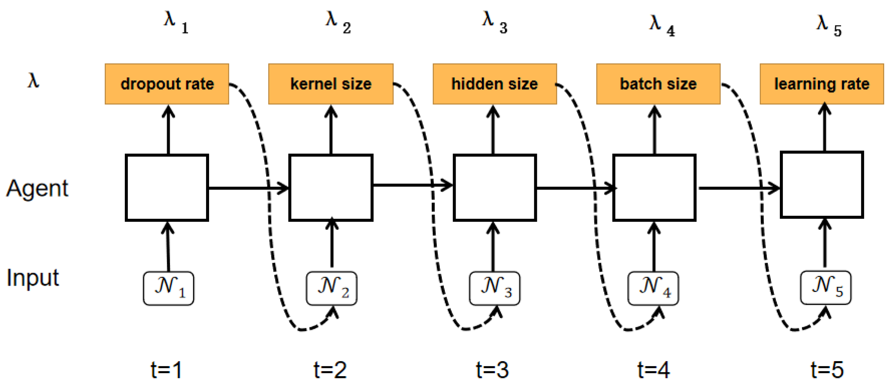
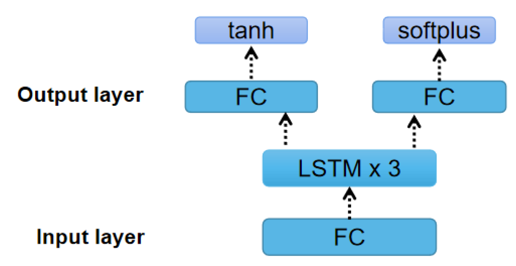
Figure 3 shows an example of the selection process for the five hyperparameters of a CNN with an agent. The initial state is randomly initialized, and then the action distribution output at each time step is used as the input for the next time step. As depicted in Figure 4, the agent consists of an input fully connected (FC) layer, three LSTM layers, and an output FC layer.

LSTM is a variant of the recurrent neural network (RNN) that solved the long-term dependency problem of vanilla RNN by using a gating system. There is a cell state $C_t$ and three gates in the LSTM cell: input gate $i_t$, output gate $o_t$, and forget gate $f_t$. The input gate $i_t$ determines how much new information is allowed to be added to the cell state; the forget gate $f_t$ determines what information is discarded from the cell state $C_t$; and the output gate $o_t$ determines what values are output. The following formulas denote the forward process of the LSTM cell:

$$\begin{array}{cc}\hfill f_t& ={\sigma }_g(W_f·[h_{t-1};x_t]+b_f)\hfill \end{array}$$

(3)

$$\begin{array}{cc}\hfill i_t& ={\sigma }_g(W_i·[h_{t-1};x_t]+b_i)\hfill \end{array}$$

(4)

$$\begin{array}{cc}\hfill o_t& ={\sigma }_g(W_o·[h_{t-1};x_t]+b_0)\hfill \end{array}$$

(5)

$$\begin{array}{cc}\hfill c_t& =f_t\odot c_{t-1}+i_t\odot \left(tanh(W_c[h_{t-1},x_t]+b_c)\right)\hfill \end{array}$$

(6)

$$\begin{array}{cc}\hfill h_t& =o_t\odot tanh\left(c_t\right)\hfill \end{array}$$

(7)

where $W_f$, $W_i$, $W_c$, $W_o$ are weight matrices and $b_f$, $b_i$, $b_c$, $b_o$ are bias vectors need to be learned. ${\sigma }_g$ and ⊙ are the sigmoid function and Hadamard product, respectively. Furthermore, $h_t$ is the hidden state and $x_t$ is the input at step t. This structure can also be extended into a multi-layer structure by leveraging the output of the last layer as the input to the next layer.

Following [15], we represent the distribution of each hyperparameter as a Gaussian distribution. Then, both the input and output of our agent are vectors containing two values: the mean $\mu$ and standard deviation $\sigma$ of the Gaussian distribution, respectively. The output at step t will be sent to the agent to obtain the result at step $t+1$. The initial input we set to the standard normal distribution. The input FC layer is used to expand the input into the same dimensions as the LSTM layer, with the aim of learning more patterns. The LSTM layer is applied to learn the temporal dependency between the steps. The output layer consists of two FC layers. After receiving the output of the LSTM layer, one of the FC layers uses the tanh function to output a value as $\mu$, while the other uses the softplus function to output $\sigma$.

3.3. Proximal Policy Optimization with Curiosity

Let $\theta$ denote the parameters of the agent, and we use the PPO-clip algorithm to update the $\theta$ in this work. As mentioned in Section 2.2, the policy gradient algorithm is difficult to select an appropriate step size. Too much difference between older and newer policies during the training process is not helpful for learning. PPO is a novel policy gradient algorithm, which can solve the issue of difficulty in determining the step length in the policy gradient algorithm. PPO algorithm introduces a new objective function that can achieve small batch update in multiple training steps. PPO-clip updates the policy with the following objective function:

$${\theta }_{k+1}=\underset{\theta }{argmax}\underset{s,a\sim {\pi }_{{\theta }_k}}{\mathbb{E}}\left[L(s,a,{\theta }_k,\theta )\right]$$

(8)

where L is given by

$$\begin{array}{cc}\hfill L(s,a,{\theta }_k,\theta )=& min(\frac{{\pi }_{\theta }\left(a\right|s)}{{\pi }_{{\theta }_k}\left(a\right|s)}{A}^{{\pi }_{{\theta }_k}}(s,a),\hfill \\ \hfill & clip(\frac{{\pi }_{\theta }\left(a\right|s)}{{\pi }_{{\theta }_k}\left(a\right|s)},1-\epsilon ,1+\epsilon )A^{{\pi }_{{\theta }_k}}(s,a))\hfill \end{array}$$

(9)

where $\epsilon$ is a hyperparameter of PPO and we set $\epsilon$ = 0.2, according to the authors’ recommendations. Let $r_t\left(\theta \right)=\frac{{\pi }_{\theta }\left(a\right|s)}{{\pi }_{\theta a_k}\left(a\right|s)}$; the PPO approach is summarized by controlling the ratio $r_t\left(\theta \right)$ of the old and new policies to prevent the change of update magnitude from affecting the agent’s learning. Clip operation will limit the value of $r_t\left(\theta \right)$ to $[1-\epsilon ,1+\epsilon ]$. Furthermore, A is the advantage function.

To solve the sparse reward problem, we use the curiosity-based prediction error method to obtain an intrinsic reward. We construct a model that receives the state $s_t$ and action $a_t$ of the current time step t and predicts the state $s_{t+1}^{{}^{\prime }}$ of the next time step $t+1$. Then, the difference between the predicted state and the true next state is used as the intrinsic reward. The agent obtains a reward $r_t$ after executing action $a_t$ at each time step. The reward $r_t$ is composed of $r_i$ and $r_e$, where $r_i$ is the intrinsic reward and $r_e$ is the environment reward. Assuming that each episode has T time steps, the $r_e$ of time steps 1 to $T-1$ is 0, while the $r_e$ of time step T is the validation set accuracy. The $r_i$ is related to the state $s_t$, the action $a_t$ of the current time step t, and the state $s_{t+1}$ of the next time step $t+1$. 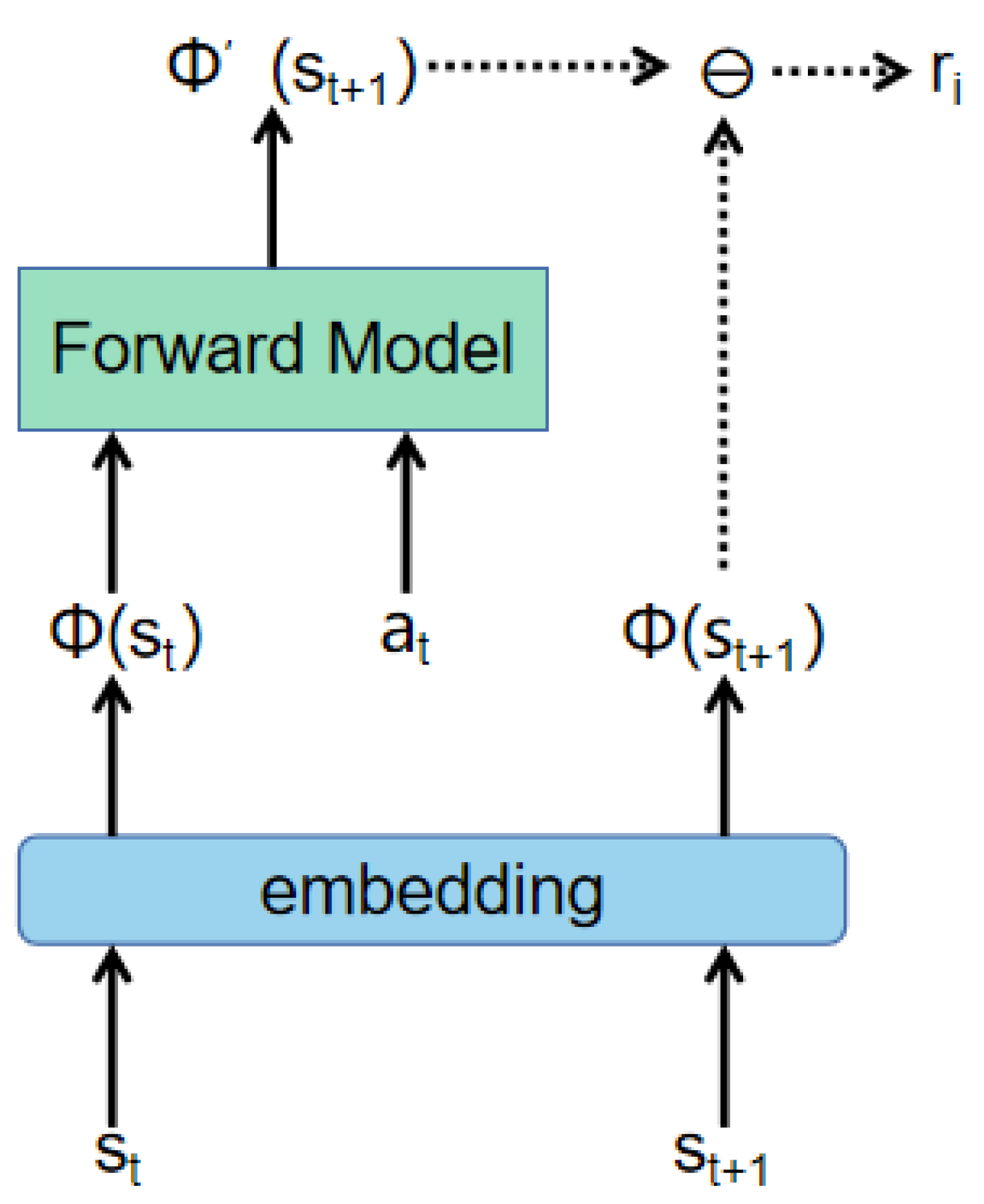Figure 5 shows how the intrinsic reward is calculated. Since each state is composed of $\mu$ and $\sigma$, we need to extend the state to a certain dimension. First, we convert $s_t$ and $s_{t+1}$ to $\Phi \left(s_t\right)$ and $\Phi \left(s_{t+1}\right)$ with an embedding layer. Then we concatenate the $\Phi \left(s_t\right)$ and $a_t$, and then feed them to the forward network to predict the ${\Phi }^{{}^{\prime }}\left(s_{t+1}\right)$. The mean squared error (MSE) between the predicted state ${\Phi }^{{}^{\prime }}\left(s_{t+1}\right)$ and the true next state $\Phi \left(s_{t+1}\right)$ is used as the intrinsic reward $r_i$ for the current time step t.

3.4. Random Forest Surrogate Model

To speed up training the agent, we use the surrogate model to establish the mapping of hyperparameter settings to the corresponding rewards. We adopt the RF algorithm to predict rewards in this work. RF belongs to the bagging algorithm in ensemble learning (EL) and has many advantages, such as determining the importance of features, determining the interaction between different features, being relatively simple to implement, etc.

Although RF can speed up the search for hyperparameters, using the surrogate model for a long time can make the agent unstable since the predicted reward is not the true accuracy after all and will produce a certain degree of bias. Therefore, we follow the works of [15] to control the adoption of the surrogate model dynamically. In the initial stage of searching, we use real rewards to update the agent. Then, we use all the obtained hyperparameter combinations and corresponding rewards as samples to train the RF algorithm and save the policy at this episode, defined as ${\pi }_{\theta }$. The KL distance of the before-and-after policy is used to control the utilization of the surrogate model dynamically. When the KL distance is less than the threshold, the surrogate model is used to predict the evaluation results of validation data set to avoid training the model. When the distance exceeds the threshold, indicating that the policy changes too much, the agent is updated by real rewards. The threshold is set to $0.1$ in this work. In this way, we can utilize surrogate models to make the search process more efficient.

3.5. Overall Framework

Algorithm 1 describes the entire process. For a given task, the agent selects hyperparameters sequentially in each episode in order, then we use the selected hyperparameters to obtain the evaluation results of the $D_{valid}$ as a reward, and finally use the PPO algorithm to update the parameters $\theta$ of the agent.

Algorithm 1 RFEPPO

Input:n: Number of hyperparameters; $s_1$: Randomly generated distributions; $\mathcal{D}$: Data set $\mathcal{D}$ = ⌀; Output: top-1 hyperparameter configuration; 1: while not done do 2:  for $i=1$ to $\frac{episodes}{2}$ do 3:   $\tau$ = [] 4:   agent selects $\lambda$ and obtains $r_T$ on $D_{valid}$ 5:   $\tau$ = [$(s_t,a_t,r_t),...,(s_T,a_T,r_T)$] 6:   use $\tau$ to update agent according to Equation (8) 7:   add $(\lambda ,r_T)$ to $\mathcal{D}$ 8:  end for 9:  Use $\mathcal{D}$ to train random forest 10:  Save the current policy $\pi$ 11:  for $\frac{episodes}{2}+1$ to $episodes$ do 12:   $\tau$ = [] 13:   agent selects $\lambda$ 14:   if $d(\pi ,{\pi }_{\theta })⩽0.1$ then 15:    use random forest to predict $r_T^{{}^{\prime }}$ 16:    $\tau$ = [$(s_t,a_t,r_t),...,(s_T,a_T,r_T^{{}^{\prime }})$] 17:    use $\tau$ to update agent according to Equation (8) 18:    add $(\lambda ,r_T^{{}^{\prime }})$ to $\mathcal{D}$ 19:   else 20:    obtain real $r_T$ on $D_{valid}$ 21:    $\tau$ = [$(s_t,a_t,r_t),...,(s_T,a_T,r_T)$] 22:    use $\tau$ to update agent according to Equation (8) 23:    add $(\lambda ,r)$ to $\mathcal{D}$ 24:   end if 25:  end for 26: end while

At the beginning of the search process, we first collect some samples of the real hyperparameter combinations $\lambda =[{\lambda }_1,{\lambda }_2,\cdots ,{\lambda }_T]$ and their corresponding validation accuracy $r_T$. After each episode, the combination of hyperparameters and corresponding accuracy $(\lambda ,r_T)$ are collected for training the surrogate model. The agent is updated at the end of each episode using the trajectory $\tau$, where $r_t$ in the trajectory is $r_i+r_e$. After the initial phase, the surrogate model is trained with the collected samples, and the policy $\pi$ is recorded at this time. In the subsequent search process, the policy ${\pi }_{\theta }$ of each episode is compared with the $\pi$, and the RL agent is updated by the intrinsic reward and real accuracy if it is greater than $0.1$; otherwise, the agent is learned by the intrinsic reward and the predicted accuracy $r_T^{{}^{\prime }}$ is made by the surrogate model. Episodes is the total number of times to search for hyperparameters.

The time complexity of searching for hyperparameters is $O(E\times t)$, where E is the number of episodes in the whole process, and t is the time required for each episode. It is worth noting that $E=E_{real}+E_{pre}$, t is divided into $t_{real}$ and $t_{pre}$, where $E_{real}$ is the number of episodes with real rewards, and $t_{real}$ is the time required for various operations in each episode at this time; $E_{pre}$ is the number of episodes with rewards predicted by the surrogate model; and $t_{pre}$ is the time required for various operations in each episode at this time. The time required to train the RF is $O(m\times log(m)\times n\times k)$, where m is the number of samples, n is the number of hyperparameters, and k is the number of decision trees. Therefore, the time complexity of the whole process is $O(E\times t+m\times log(m)\times n\times k)$.

4. Experiments

In this section, to evaluate our proposed RFEPPO method, we use it to optimize the hyperparameters of XGBoost and CNN. Among them, XGBoost is a common algorithm for handling tabular data, while CNN is a typical model for processing image data. We first introduce the experimental setup, present the datasets, the conventional approaches, and the evaluation method. Then we conduct comparison experiments on tabular and image datasets to compare our method with conventional methods. Finally, to verify the effect of the components in our method on the HPO results, we perform ablation experiments.

For fairness, all search algorithms ran on Intel Core i9-11900K CPU. The XGBoost algorithm also ran on the CPU. To save time, we used a single NVIDIA GeForce RTX 3090 GPU when training the CNN model.

4.1. Experimental Setup

Datasets: We validated our method on 11 datasets, 9 of which are tabular data to verify the performance of RFEPPO tuning the hyperparameters of XGBoost, and the remaining two image datasets to verify the performance tuning the hyperparameters of CNN.

Table 1. Details of datasets.

Default Task	Datasets	#Instances	#Attributtes
Multi Classification	winequality_white	4898	11
	optdigits	5620	64
	Turkiye_Student_Evaluation	5820	28
	balance_scale	625	4
	Cardiotocography	2126	21
Binary Classification	monks_1	556	6
	DR_Debrecen	1151	19
	churn	5000	20
	socmob	1156	5
Image Classification	MNIST	70,000	$28\times 28\times 1$
	Fashion_MNIST	70,000	$28\times 28\times 1$

shows the details of the datasets.

The tabular datasets are from the UCI Machine Learning Repository [31] and openML [32]. These datasets come from different fields, including computer, medicine, education, life, and physics. The MNIST dataset [33] and Fashion MNIST dataset [34] are classic image classification datasets in the field of ML. Both of them consist of 60,000 training samples and 10,000 test samples, each of which is a $28\times 28$ pixel grayscale image. Fashion MNIST is identical to the original MNIST in training set/test set division, size and format.

For the tabular datasets, we divide each dataset into training, validation and test set by a ratio of $6:2:2$; for the image datasets, we follow the original split ratio and then use the last 5000 samples of the training set as the validation set.

Comparison Methods: In this paper, we compared our approach with the following optimization algorithms: RS [6], TPE [5], hyperband [1], BOHB [12], and the default configuration of XGBoost (baseline). In this paper, we implemented these algorithms with the Hyperopt and HpBandSter Libraries. In addition, we also compared our method with the MBRL-SDP model proposed in the [15]. RS randomly selects samples within the search range. By random sampling, the global optimum or its approximation can also be searched with high probability if the set of samples is sufficiently large.TPE is a sequential model-based optimization (SMBO) method that tries to build a probabilistic model of the function at each step and selects the most promising parameters for the next step. Hyperband attempts to explore as many configurations as possible with limited resources and returns the most probable configuration as a final result. The weakness of hyperband is generating new configurations randomly without leveraging finished trials. BOHB is a follow-up work to hyperband, which generates a certain percentage of new configurations by constructing multiple TPE models to take advantage of the finished trials.

Evaluation metrics: The performance of HPO methods are evaluated using the following metrics:

• Time: average search time required to search 200 episodes per method.
• Accuracy: average accuracy of each method in the test set.

Details: As presented in Section 3.2, the agent consists of an input FC layer, three LSTM layers with hidden state size of 128, and an output FC layer. The learning rate of the agent is set to $0.001$. The rest of the settings are configured using the default configuration of the PPO algorithm. Before using the surrogate model RF, we adopted grid search to find the best hyperparameters for RF. The accuracy of the validation set is collected for the first 100 episodes, and then the combination of hyperparameters and accuracy from these 100 episodes are used as samples to train the RF. The KL distance threshold between policies is set to $0.1$. For the curiosity model, the embedding layer captures state information and extends the state to 32 dimensions. The input of the forward network is the action and the state after embedding, and the middle layer is a fully connected layer with hidden_size of 64. Since the prediction error is calculated with the next true state, the output layer size of the forward network is also 32.

In this experiment, we ran each method five times and the budget for each run was training 200 episodes. For the five best configurations output from five trials, the average of the corresponding test set accuracy is compared.

4.2. Performance Evaluation

4.2.1. HPO for XGBoost

XGBoost is derived from the gradient boosting framework. It is more efficient because of the algorithm’s parallel computation, approximate tree building, efficient handling of sparse data, and memory usage optimization, which make it at least 10 times faster than the existing gradient boosting implementations. XGBoost can handle many tasks, such as regression, classification, and sorting.

Search Space: We consider the 10 hyperparameters of XGBoost as shown in

Table 2. Hyperparameters of XGBoost.

Name	Type	Ranges
max_depth	int	$[1,25]$
learning_rate	float	$[0.001,0.1]$
n_estimators	int	$[50,1200]$
gamma	float	$[0.05,0.9]$
min_child_weight	int	$[1,9]$
subsample	float	$[0.5,1]$
colsample_bytree	float	$[0.5,1]$
colsample_bylevel	float	$[0.5,1]$
reg_alpha	float	$[0.1,0.9]$
reg_lambda	float	$[0.01,0.1]$

. We ran experiments with XGBoost on nine classification datasets, and

Table 3. The performance (mean ± std) of our method and other conventional algorithms on nine tabular datasets.

Data Set	RS		TPE		Hyperband		BOHB
	Acc (%)	Time (s)	Acc (%)	Time (s)	Acc (%)	Time (s)	Acc (%)	Time (s)
winequality_white	64.86 ± 2.12	479 ± 16	66.35 ± 0.75	518 ± 101	67.10 ± 0.51	137 ± 7	62.24 ± 0.40	124 ± 5
optdigits	97.79 ± 0.33	506 ± 12	97.85 ± 0.34	493 ± 65	98.17 ± 0.37	129 ± 7	98.10 ± 0.13	120 ± 3
Turkiye_Student_Evaluation	85.46 ± 0.94	313 ± 15	86.67 ± 0.33	315 ± 79	86.92 ± 0.52	73 ± 3	87.03 ± 0.38	72 ± 2
balance_scale	89.92 ± 1.18	48 ± 1	91.52 ± 0.64	57 ± 9	91.04 ± 0.93	17 ± 0	92.48 ± 0.96	20 ± 0
Cardiotocography	88.45 ± 1.65	263 ± 7	87.09 ± 0.42	273 ± 33	87.32 ± 0.15	80 ± 2	88.03 ± 0.66	63 ± 1
monks_1	96.07 ± 1.84	20 ± 0	95.54 ± 1.69	26 ± 2	97.32 ± 0.00	9 ± 1	90.36 ± 6.79	9 ± 0
DR_Debrecen	70.04 ± 2.81	41 ± 1	70.13 ± 1.52	45 ± 5	69.18 ± 0.50	14 ± 1	71.26 ± 0.89	13 ± 0
churn	95.58 ± 0.89	89 ± 3	94.60 ± 0.23	106 ± 8	96.08 ± 0.07	25 ± 1	95.86 ± 0.29	27 ± 0
socmob	93.71 ± 1.11	22 ± 0	93.62 ± 0.74	28 ± 3	92.07 ± 0.58	9 ± 1	94.31 ± 1.37	5 ± 0
Average values	86.88 ± 1.43	198 ± 6	87.04 ± 0.74	236 ± 34	87.24 ± 0.40	55 ± 2	86.63 ± 1.32	50 ± 1
Data Set	MBRL-SDP		RFEPPO (Our Method)		Baseline
	Acc (%)	Time (s)	Acc (%)	Time (s)	Acc (%)	Time (s)
winequality_white	65.40 ± 0.87	397 ± 44	67.84 ± 0.40	420 ± 187	65.25 ± 1.29	-
optdigits	97.44 ± 0.69	370 ± 169	98.35 ± 0.18	408 ± 146	97.59 ± 0.39	-
Turkiye_Student_Evaluation	85.98 ± 0.80	298 ± 99	87.87 ± 0.37	253 ± 81	84.69 ± 1.44	-
balance_scale	90.88 ± 1.09	143 ± 9	92.67 ± 0.64	150 ± 2	86.24 ± 0.93	-
Cardiotocography	87.42 ± 1.25	223 ± 35	89.39 ± 0.27	252 ± 70	86.99 ± 0.19	-
monks_1	96.25 ± 1.64	139 ± 5	98.57 ± 0.44	136 ± 6	98.39 ± 0.87	-
DR_Debrecen	67.00 ± 3.48	142 ± 4	74.72 ± 1.49	152 ± 15	68.13 ± 2.85	-
churn	95.58 ± 0.40	163 ± 17	96.38 ± 0.30	169 ± 6	95.83 ± 0.71	-
socmob	93.88 ± 0.57	136 ± 6	96.55 ± 0.39	137 ± 5	93.87 ± 1.03	-
Average values	86.65 ± 1.20	223 ± 43	89.15 ± 0.50	228 ± 58	86.33 ± 1.08	-

shows the performance.

Results: We ran each method five times, and the average search time and accuracy on the test set are tabulated in Table 3. It can be seen that RFEPPO outperforms other optimization methods and baseline in terms of accuracy. The accuracy of our method is substantially higher than the baseline, which indicates the importance of HPO. For the search time, hyperband and BOHB spend the least time on all datasets due to the fact that the bandit-based approach would use a very small budget in the initial stage and would quickly discard the poorly performing hyperparameter configurations. However, for the accuracy, both BOHB and hyperband are lower than our method. We believe that BOHB and hyperband may throw away the hyperparameter configurations that really perform well in the initial stage. Compared to RS and TPE, our method can reduce the time by about 27% to 40% on winequality_white, optdigits and Turkiye_Student_Evalution datasets, and reduce the time by about 4% on the Cardiotocography dataset. For other datasets, the search time of our method is a little slower. However, the accuracy on test set of our method is better than all other methods. This shows that our method has a clear advantage for datasets with a large sample size and a large number of features. Although the search time of our method is slower for small datasets, the accuracy is higher than other methods. In addition, compared to MBRL-SDP, our method has higher accuracy in the test set. This demonstrates that intrinsic reward can encourage the exploration of novel states and thus quickly find well-performing hyperparameter configurations.

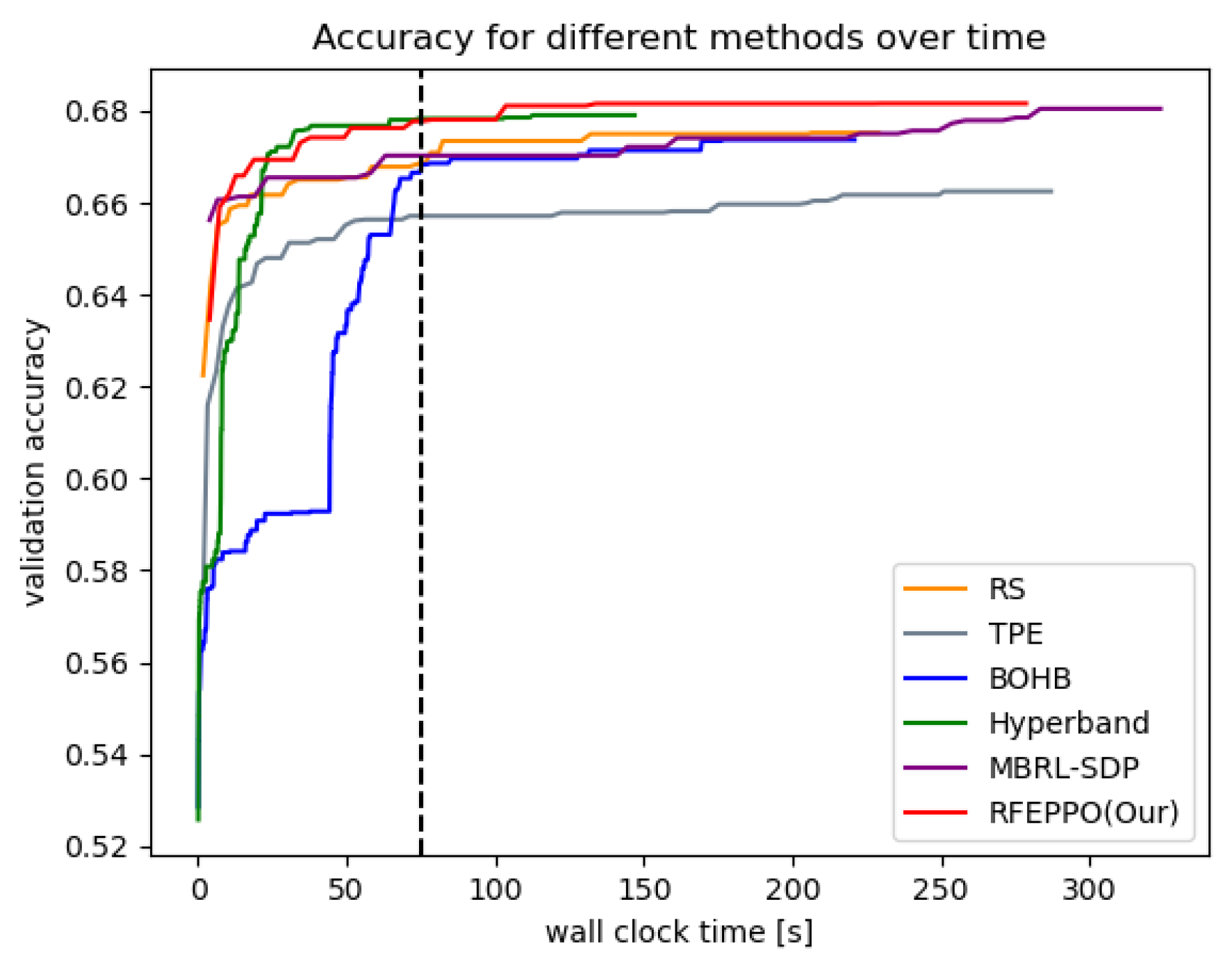
To verify the effectiveness of RFEPPO, we visualize the performance curve as the validation accuracy of all methods over a period of wall clock time. Figure 6 compares RFEPPO with all methods on the winequality_white dataset. From the figure, we can see that our method can find good hyperparameter configurations faster and performs better overall compared to MBRL-SDP and RS. As can be seen by the left part of the black line, our method can achieve similar performance to hyperband, and is initially slightly faster than it. Although TPE also converges quickly in the initial stage, the final performance is worse than RFEPPO. This experiment demonstrates that our method not only shortens the search time on large datasets, but also improves the accuracy and reliability of the tasks.

4.2.2. HPO for CNN

In this experiment, we try to optimize the hyperparameters of the LeNet [35] automatically. The LeNet-5 designed for handwritten font recognition is one of the most popular CNN models. LeNet-5 saves a lot of computational cost by cleverly designing the network to extract features using convolution operation, parameter sharing, and pooling, then using an FC layer for classification recognition. Moreover, many recent novel CNN models are inspired by this network structure.

Search Space: We consider the five hyperparameters of LeNet as shown in

Table 4. Hyperparameters of LeNet.

Name	Type	Ranges
conv_size	int	$[2,7]$
hidden_size	int	$[124,1024]$
batch_size	int	$[16,32]$
dropout_rate	float	$[0.5,0.9]$
learning_rate	float	$[0.0001,0.1]$

. Experiments were carried with LeNet on MNIST and Fashion MNIST datasets, which are commonly used to test the performance of ML and DL models.

Results: The results for average accuracy and search time of our method and other conventional methods are tabulated in

Table 5. The performance (mean ± std) of our method and other conventional algorithms on 2 image datasets.

Datasets	RS		TPE		Hyperband
	Acc (%)	Time (h)	Acc (%)	Time (h)	Acc (%)	Time (h)
MNIST	99.17 ± 0.14	1.48 ± 0.013	99.19 ± 0.06	1.46 ± 0.051	98.82 ± 0.07	1.04 ± 0.050
Fashion_MNIST	90.56 ± 0.59	1.48 ± 0.016	91.70 ± 0.24	1.53 ± 0.040	86.85 ± 1.29	0.98 ± 0.004
Datasets	BOHB		MBRL-SDP		RFEPPO (Our Method)
	Acc (%)	Time (h)	Acc (%)	Time (h)	Acc (%)	Time (h)
MNIST	99.10 ± 0.02	0.94 ± 0.046	99.24 ± 0.04	0.76 ± 0.010	99.33 ± 0.05	0.75 ± 0.002
Fashion_MNIST	90.78 ± 0.40	0.92 ± 0.013	89.91 ± 0.04	0.76 ± 0.003	92.16 ± 0.27	0.78 ± 0.014

. As can be seen in this table, our method outperforms other methods in terms of accuracy and time. The search time is greatly reduced since utilizing the surrogate model. Among RS, TPE, hyperband and BOHB, for MNIST and Fashion MNIST datasets, BOHB takes the shortest time, and TPE has the highest accuracy. Compared to BOHB, our method can reduce the time by about 15% to 20%, demonstrating that the surrogate model can reduce the search time. For MBRL-SDP, although its time is similar to our method on these two datasets, it does not perform well on the test set. This also illustrates the effectiveness of intrinsic reward. This experiment demonstrates that our method not only achieves high accuracy on large datasets, but also requires much less time.

Figure 7 shows the best validation set accuracy over time for all methods on the MNIST dataset. Each method was run five times and the average of the five accuracy was calculated. By observing the black line, we can see that our method can find a good hyperparameter configuration much faster compared to MBRL-SDP. Since hyperband and BOHB use a small budget (e.g., epoch) in the initial stage, these two methods will run multiple sets of hyperparameter configurations initially, and it is possible to find hyperparameter configurations that perform well. Therefore the speed of finding good configurations is faster than our method. Although TPE and our method will find good configurations simultaneously, our method converges faster in the initial stage. Moreover, our method has significant advantages over RS and MBRL-SDP. This experiment demonstrates that RFEPPO not only achieves high accuracy on large datasets, but also requires much less time.

4.3. Ablation Experiments

In this section, first we compare the performance with and without the curiosity-driven method, then compare the performance with different RL algorithms, and next we compare the performance with and without the surrogate model. Finally, we replace RF with other conventional regression models and compare the performance of these different algorithms.

4.3.1. Performance Comparison with and without Curiosity-Driven Method

To demonstrate that the addition of intrinsic reward has a better effect and can improve accuracy in the test set, we removed the curiosity mechanism and only used the validation set accuracy as reward. We conducted comparison experiments on the balance_scale data set.

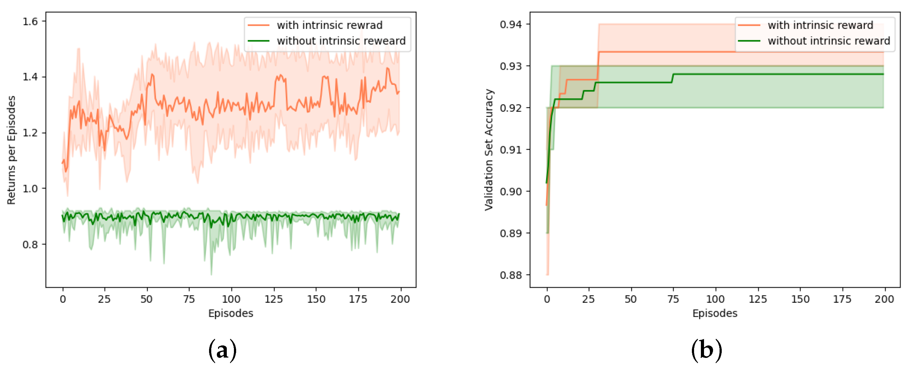
Figure 8 shows the effect of intrinsic reward on the overall search process. In Figure 8a, the green line refers to the reward return for each episode using only the accuracy of the validation set as the reward. We can find that the agent’s reward has no obvious upward trend with the growth of episodes. We believe that the reason for this phenomenon is that the agent is updated slowly due to too many sparse rewards and little sample utilization. Moreover, better validation set accuracy is obtained at the initial stage of the search process, which we believe is caused by the suitability of the initial state of this dataset. The coral line refers to the reward return for each episode when using the intrinsic reward. We can find an overall upward trend in the reward return for the whole search process. This is because the curiosity-driven method encourages the agent to explore more unfamiliar states, and the more novel the state, the higher the intrinsic reward. The use of intrinsic reward improves the utilization of the sample, which allows the agent to learn more about the environment. Figure 8b shows the accuracy of the validation set corresponding to the best hyperparameter configuration searched in the current episode. We can see that compared to the non-intrinsic reward approach, the use of the intrinsic reward approach can find high-performance hyperparameter configuration quickly and with higher accuracy. Therefore, we believe that intrinsic reward can solve the problem of sparse reward in HPO. The curiosity-driven method encourages the agent to keep exploring unfamiliar states, and finds better hyperparameter configurations faster.

4.3.2. Performance Comparison with Different RL Algorithms

To verify the effectiveness of PPO used in this experiment, we replaced PPO with other RL algorithms. In this experiment, we did not use the intrinsic reward and surrogate model, and performed comparisons on nine tabular datasets by replacing PPO with advantage actor–critic (A2C), deep deterministic policy gradient (DDPG) [36], soft actor–critic (SAC) [37], and twin delayed DDPG (TD3) [38]. For A2C, DDPG and SAC, we set the hidden size to a range of $\{32,64,128\}$. For TD3, we set the exploration noise scale to a range of $\{0.5,1\}$ and the delay update frequency to a range of $\{3,4,5\}$. The hyperparameters of these RL algorithms were determined by the grid search within their respective ranges, ensuring the final model performance.

Table 6. The performance (mean ± std) of our method with different RL algorithms.

Datasets	A2C		DDPG		SAC		TD3		PPO
	Acc (%)	Time (s)	Acc (%)	Time (s)	Acc (%)	Time (s)	Acc (%)	Time (s)	Acc (%)	Time (s)
winequality_white	67.03 ± 1.60	479 ± 29	66.73 ± 1.62	420 ± 192	67.38 ± 1.40	530 ± 4	67.34 ± 2.15	422 ± 52	0.6837 ± 0.89	548 ± 34
optdigits	98.45 ± 0.40	508 ± 21	98.40 ± 0.24	459 ± 177	98.29 ± 0.26	576 ± 16	98.47 ± 0.75	403 ± 42	0.9855 ± 0.29	580 ± 11
Turkiye_Student_Evaluation	87.67 ± 0.47	334 ± 14	87.65 ± 0.19	154 ± 3	87.60 ± 0.74	378 ± 6	87.52 ± 0.47	292 ± 56	0.8763 ± 1.30	363 ± 16
balance_scale	92.54 ± 0.96	67 ± 2	92.58 ± 1.09	89 ± 22	92.80 ± 2.24	112 ± 2	93.31 ± 0.60	71 ± 9	0.9367 ± 1.28	103 ± 1
Cardiotocography	89.47 ± 1.33	262 ± 6	89.00 ± 1.26	299 ± 57	89.36 ± 1.91	316 ± 18	88.92 ± 0.58	245 ± 22	0.8904 ± 0.82	296 ± 2
monks_1	99.39 ± 1.64	39 ± 1	98.86 ± 2.44	63 ± 0	99.18 ± 0.87	83 ± 2	99.64 ± 0.87	58 ± 2	0.9970 ± 1.21	77 ± 1
DR_Debrecen	73.06 ± 1.88	59 ± 2	72.73 ± 2.00	72 ± 2	73.38 ± 1.87	105 ± 3	73.66 ± 3.63	73 ± 1	0.7301 ± 2.39	98 ± 0
churn	96.42 ± 0.34	130 ± 30	96.21 ± 0.62	135 ± 44	96.40 ± 0.32	156 ± 2	96.42 ± 0.69	91 ± 19	0.9643 ± 0.95	151 ± 1
socmob	96.12 ± 2.29	41 ± 1	96.21 ± 0.47	62 ± 8	96.40 ± 1.72	85 ± 0	95.76 ± 1.64	64 ± 10	0.9598 ± 1.20	78 ± 0

shows the accuracy and search time of the five sets of experiments. We ran each method five times, and trained 200 episodes each time.

As can be seen from Table 6, the highest accuracy is achieved on most of the datasets using the PPO algorithm, while other algorithms can only achieve the highest accuracy on one data set. DDPG has the lowest accuracy on all datasets. However, in terms of search time, PPO is slower than other algorithms. A2C has a relatively fast search time on small datasets, DDPG and TD3 have a relatively fast search time on large datasets, but none of the corresponding accuracies is the highest. Therefore, for the task of HPO, we believe that PPO is more effective than other RL algorithms.

4.3.3. Performance Comparison with Surrogate Model and without Surrogate Model

To verify the effectiveness of the surrogate model, we removed the RF surrogate model in RFEPPO and compared it with our method. In this experiment, we performed comparisons on nine tabular datasets.

Table 7. The performance (mean ± std) of PPO with surrogate model and without surrogate model.

Datasets	Without Surrogate Model	With Surrogate Model
	Acc (%)	Time (s)	Acc (%)	Time (s)
winequality_white	67.81 ± 1.07	553 ± 109	67.84 ± 0.40	420 ± 187
optdigits	98.31 ± 0.15	659 ± 256	98.35 ± 0.18	408 ± 146
Turkiye_Student_Evaluation	87.85 ± 0.26	379 ± 172	87.87 ± 0.37	253 ± 81
balance_scale	92.16 ± 0.32	193 ± 17	92.67 ± 0.64	150 ± 2
Cardiotocography	89.42 ± 0.59	363 ± 141	89.39 ± 0.27	252 ± 70
monks_1	98.04 ± 0.67	149 ± 10	98.57 ± 0.44	136 ± 6
DR_Debrecen	72.90 ± 0.59	185 ± 11	74.72 ± 1.49	152 ± 15
churn	96.42 ± 0.29	204 ± 43	96.38 ± 0.30	168 ± 6
socmob	95.78 ± 0.92	149 ± 11	96.55 ± 0.39	137 ± 5

shows the accuracy and search time of the two sets of experiments. Each method was run five times and trained 200 episodes each time.

As can be seen from Table 7, the time spent is reduced after adding the surrogate model. This indicates that the predicted accuracy of the surrogate model is used to update the agent during the search, making part of the process without actually training XGBoost, which ultimately reduced the time. Additionally, seven of the nine datasets also show an increase in accuracy after adding the surrogate model. Thus, this demonstrates that the inclusion of the surrogate model speeds up the search without affecting the accuracy of the test set.

4.3.4. Performance Comparison with Different Surrogate Models

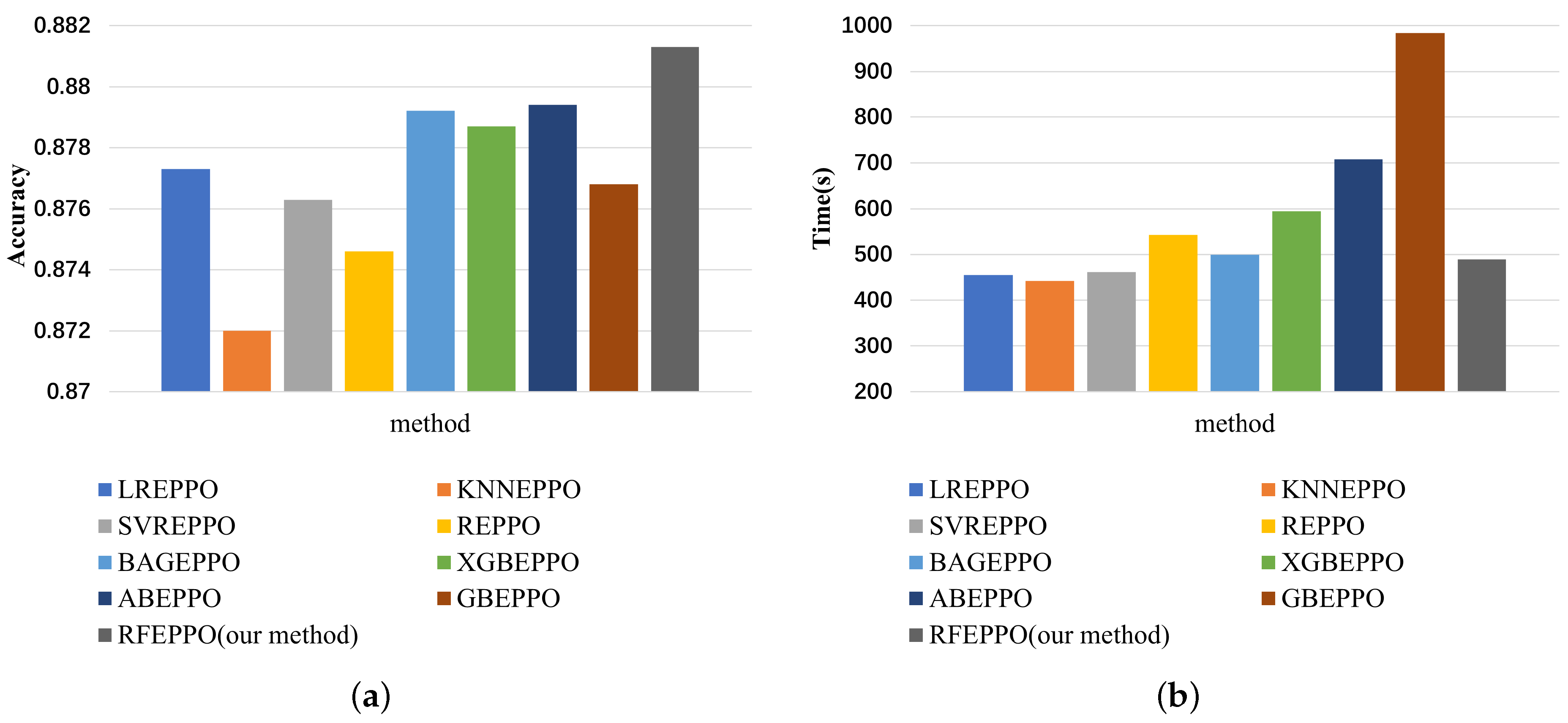
To verify the effectiveness of RF in our approach, we replaced RF in RFEPPO with other common ML methods and compared them. Since the surrogate model in our method can be replaced with other regression models arbitrarily, we compared our method with LREPPO, KNNEPPO, SVRPPO, REPPO, BAGEPPO, XGBEPPO, ABEPPO, and GBEPPO, which replace RF in RFEPPO with linear regression, KNN, SVR, Ridge, Bagging, XGBoost, AdaBoost, and gradient boost, respectively. For KNN, we set the number of neighbors and the power parameter to a range of $\{2,3,4,5,6\}$ and $\{1,2\}$ respectively. For SVR, we used the radial basis function (RBF) kernel. For ridge, we set regularization strength among $\{0,0.01,0.1,1\}$. For bagging, XGBoost, AdaBoost, gradient boost and RF, we set the number of decision trees among $\{100,110,\cdots ,200\}$. The hyperparameters of these methods were determined by the grid search within their respective ranges, ensuring the final model performance. In this experiment, we chose the Turkiye Student Evaluation dataset for validation. As in previous experiments, we ran each method five times and trained 200 episodes each time. The accuracy and time for each method are shown in Figure 9. From this figure, it can be seen that RF has better final accuracy than other models. Although LREPPO, KNNEPPO, and SVRPPO take less time than RFEPPO, the cost of using them is reduced accuracy. Other methods are worse than RF in terms of both time and accuracy. Therefore, we believe that RF is the most suitable surrogate model in our method.

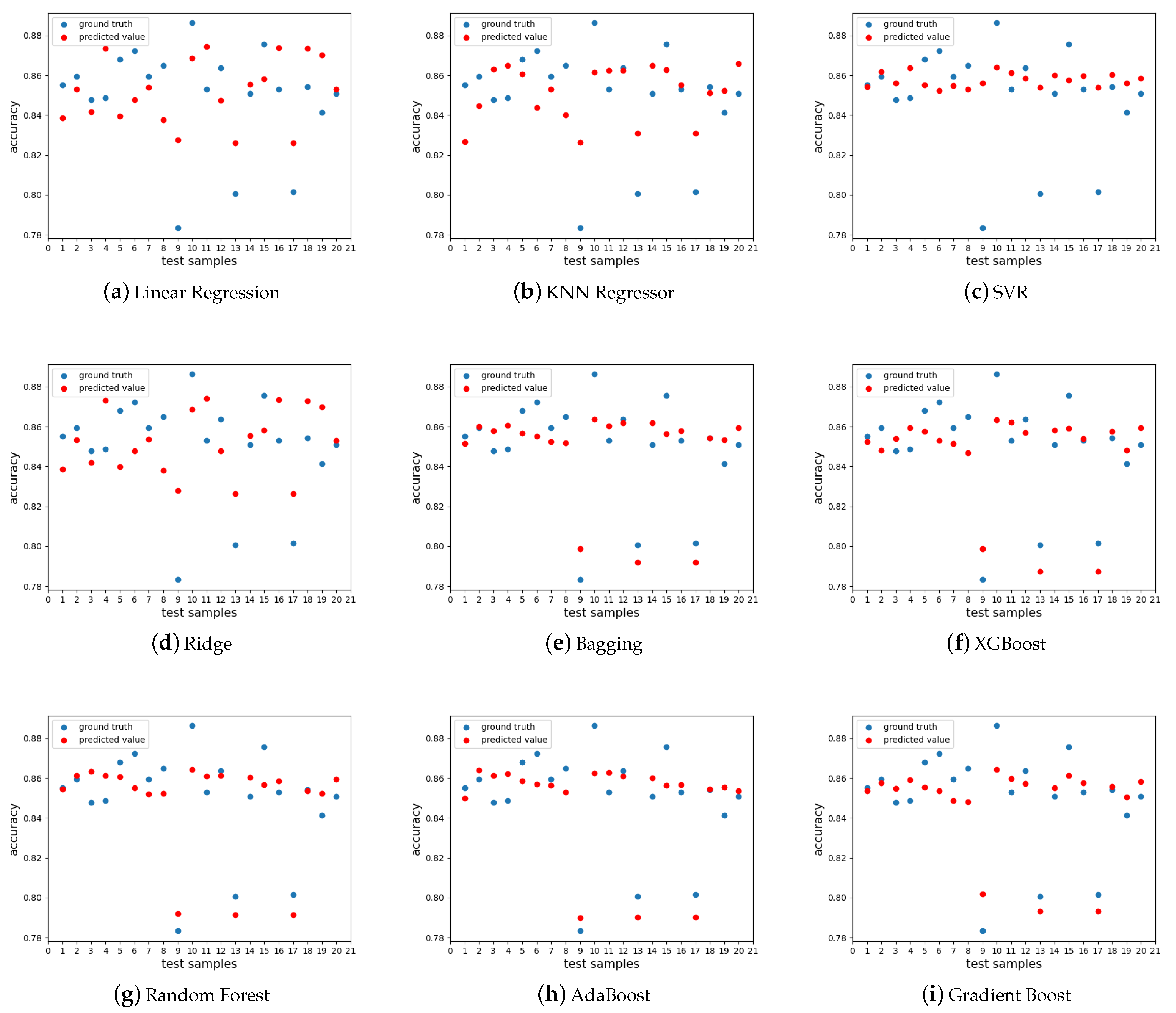
In order to further analyze the RF surrogate model, we need to know its predictive performance, thus we collected 100 samples from the first 100 episodes. Each sample was a combination of hyperparameters and the corresponding accuracy of validation set. To compare the performance of these surrogate models, the 100 samples were divided into training and testing samples in the ratio of 8:2. The RMSE results of the test samples are tabulated in

Table 8. RMSE results of different surrogate models on the test samples set.

Method	RMSE
Linear Regression	0.0216
KNN Regressor	0.0201
SVR	0.0258
Ridge	0.0216
Bagging	0.0111
XGBoost	0.0120
AdaBoost	0.0107
Gradient Boost	0.0112
RandomForest	0.0105

, and the ground truth of the test samples and the predicted results of each model are presented in the Figure 10. It is obvious from Table 8 that RF performs the best. In Figure 10, the blue points represent the true values and the red points represent the predicted results. Moreover, we can see that the ensemble methods, bagging, RF, XGBoost, Adaboost, and gradient boost, perform better than the remaining methods.

4.4. Discussion

This paper focuses on the HPO problem and proposes an RL-based approach. First, we treated the HPO problem as a sequential decision process and model it as MDP. Then, we designed an agent to select the hyperparameters sequentially and be updated by PPO. In order to mitigate sparse rewards problem, the curiosity-driven approach was used to provide intrinsic rewards. Additionally, we adopted RF as a surrogate model to reduce the search time. We validated our method on multi-classification, binary classification and image datasets. The accuracy of our method is better than other methods on all datasets. Our proposed method does not take less time than bandit-based methods when processing tabular data, but we have a significant improvement in search efficiency when processing image data. We believe that our approach is more efficient than bandit-based methods in the case of relatively large dataset sizes and long model training times. The reason is that bandit-based methods have to train the model with all candidate hyperparameter combinations for at least one epoch in the initial stage, while our method avoids the process of training the model many times by using the surrogate model.

In our future work, we will focus on two research directions. First, we will study how to optimize the hyperparameters of models that accomplish more complex tasks, such as object detection and sentiment analysis, which have been widely studied recently. Second, we will study how to accomplish model generation and HPO simultaneously, and eventually develop a complete automatic ML framework.

5. Conclusions

HPO plays a vital role in ML and DL models. In this paper, we propose a novel RFEPPO algorithm to solve the HPO problem. We consider the selection of hyperparameters as a sequential decision problem, and use the agent to sequentially select hyperparameters which is updated with the PPO based algorithm with surrogate model. The proposed method is validated on nine tabular datasets and two image datasets. The experiment results indicate that the proposed RFEPPO outperforms RS, TPE, hyperband, and BOHB.