
Plant Disease Detection Using Deep Convolutional Neural Network

 ,
,  ,
,  ,
,  ,
, 
Abstract
:1. Introduction
2. Related Works
3. Materials and Methods
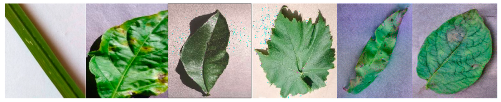
3.1. Dataset Preparation and Preprocessing
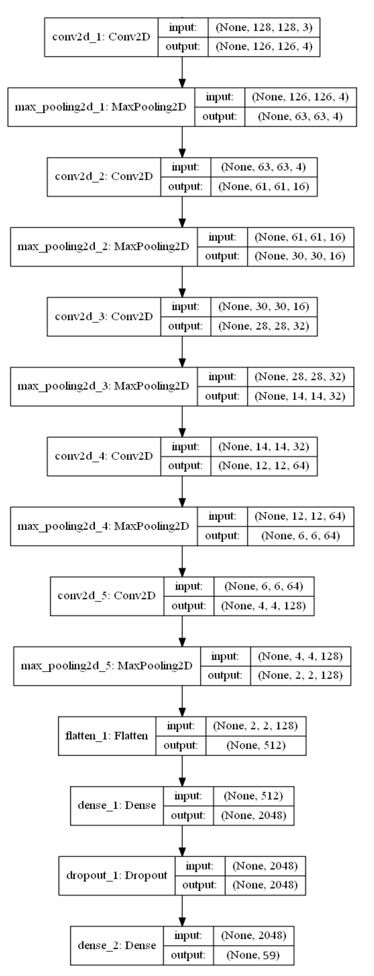
3.2. Model Design
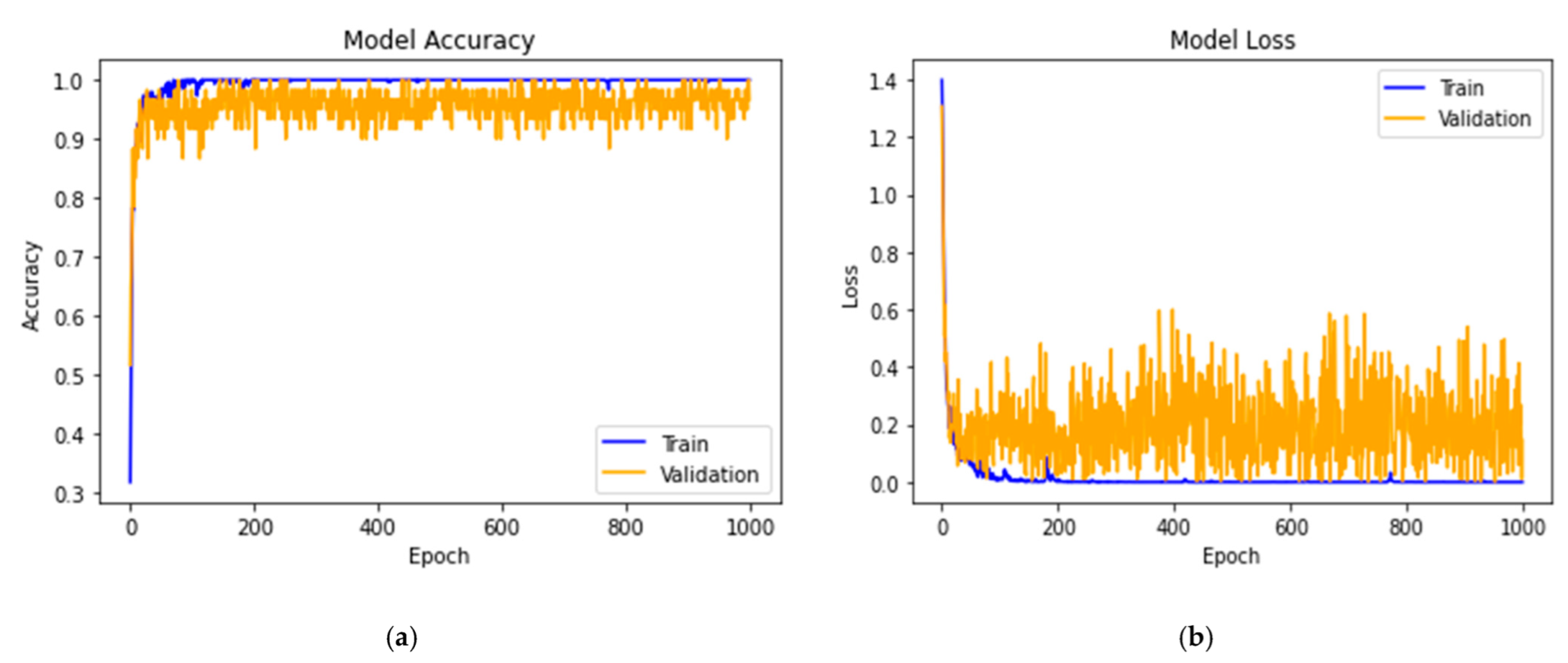
3.3. Model Training
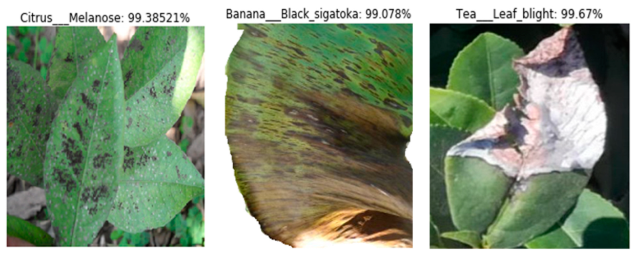
3.4. Model Prediction
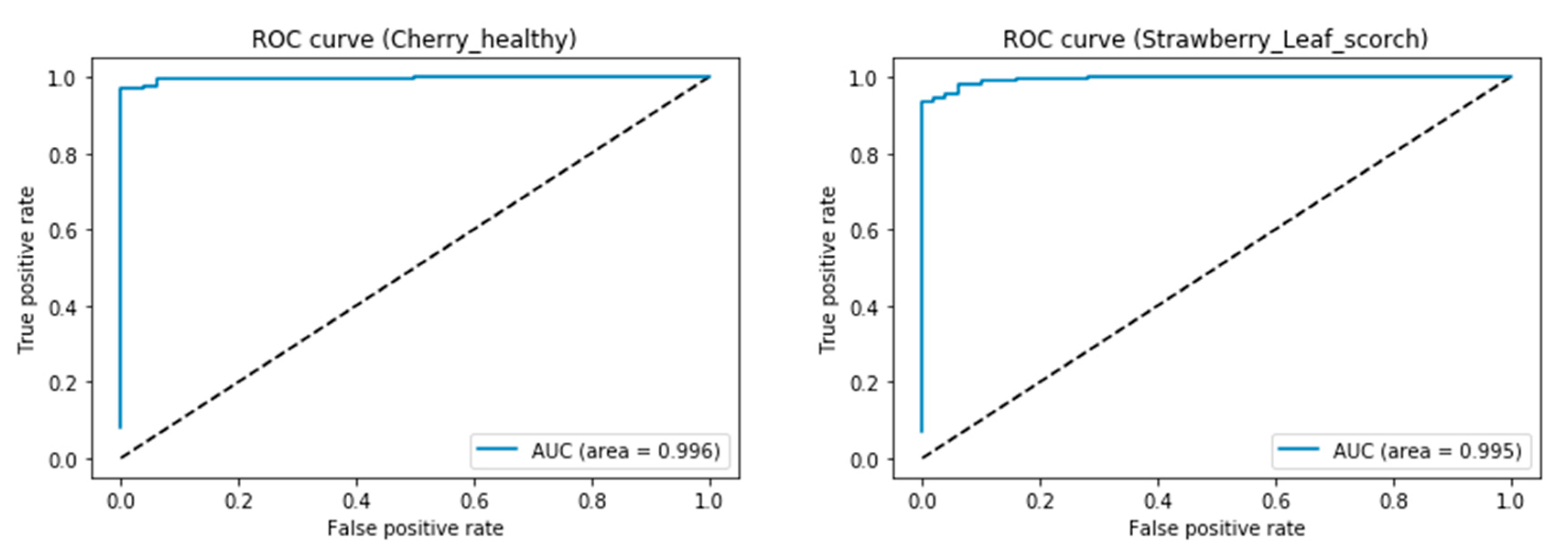
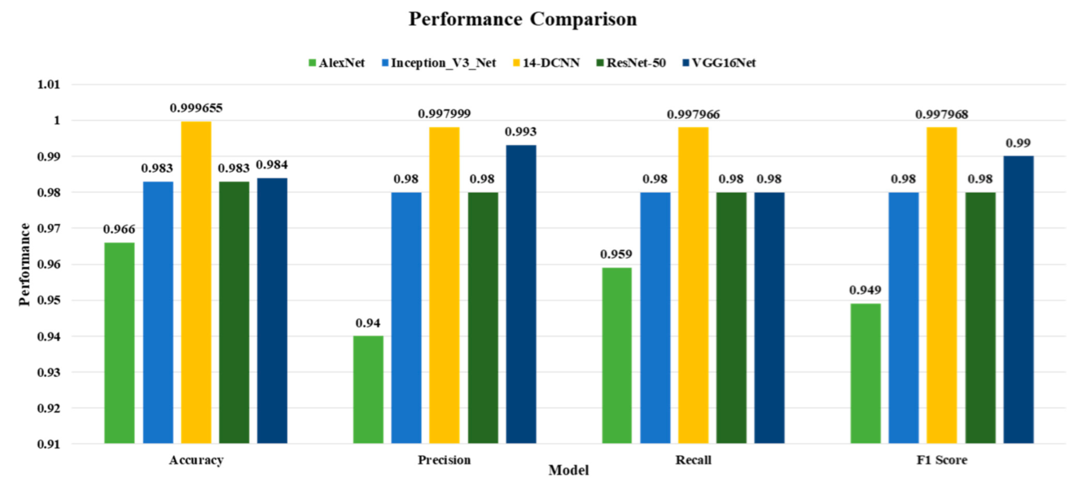
4. Results
5. Conclusions
Author Contributions
Funding
Institutional Review Board Statement
Informed Consent Statement
Data Availability Statement
Conflicts of Interest
References
- Pandian, J.A.; Kanchanadevi, K.; Kumar, V.D.; Jasińska, E.; Goňo, R.; Leonowicz, Z.; Jasiński, M. A Five Convolutional Layer Deep Convolutional Neural Network for Plant Leaf Disease Detection. Electronics 2022, 11, 1266. [Google Scholar] [CrossRef]
- Sladojevic, S.; Arsenovic, M.; Anderla, A.; Culibrk, D.; Stefanovic, D. Deep Neural Networks Based Recognition of Plant Diseases by Leaf Image Classification. Comput. Intell. Neurosci. 2016, 2016, 3289801. [Google Scholar] [CrossRef] [Green Version]
- Geetharamani, G.; Pandian, A. Identification of plant leaf diseases using a nine-layer deep convolutional neural network. Comput. Electr. Eng. 2019, 76, 323–338. [Google Scholar]
- Rumpf, T.; Mahlein, A.-K.; Steiner, U.; Oerke, E.-C.; Dehne, H.-W.; Plümer, L. Early detection and classification of plant diseases with Support Vector Machines based on hyperspectral reflectance. Comput. Electron. Agric. 2010, 74, 91–99. [Google Scholar] [CrossRef]
- Chen, H.-C.; Widodo, A.M.; Wisnujati, A.; Rahaman, M.; Lin, J.C.-W.; Chen, L.; Weng, C.-E. AlexNet Convolutional Neural Network for Disease Detection and Classification of Tomato Leaf. Electronics 2022, 11, 951. [Google Scholar] [CrossRef]
- Lee, S.H.; Chan, C.S.; Wilkin, P.; Remagnino, P. Deep-plant: Plant identification with convolutional neural networks. In Proceedings of the 2015 IEEE International Conference on Image Processing (ICIP), Quebec City, QC, Canada, 27–30 September 2015; pp. 452–456. [Google Scholar]
- Brahimi, M.; Arsenovic, M.; Laraba, S.; Sladojevic, S.; Boukhalfa, K.; Moussaoui, A. Deep Learning for Plant Diseases: Detection and Saliency Map Visualisation. In Human and Machine Learning: Visible, Explainable, Trustworthy and Transparent; Zhou, J., Chen, F., Eds.; Springer International Publishing: Cham, Switzerland, 2018; pp. 93–117. [Google Scholar]
- Ferentinos, K.P. Deep learning models for plant disease detection and diagnosis. Comput. Electron. Agric. 2018, 145, 311–318. [Google Scholar] [CrossRef]
- Arun Pandian, J.; Geetharamani, G. Data for: Identification of Plant Leaf Diseases Using a 9-Layer Deep Convolutional Neural Network. Mendeley Data. 2019. Available online: https://data.mendeley.com/datasets/tywbtsjrjv/1 (accessed on 29 March 2020).
- Almadhor, A.; Rauf, H.T.; Lali, M.I.U.; Damaševičius, R.; Alouffi, B.; Alharbi, A. AI-Driven Framework for Recognition of Guava Plant Diseases through Machine Learning from DSLR Camera Sensor Based High Resolution Imagery. Sensors 2021, 21, 3830. [Google Scholar] [CrossRef]
- Shijie, J.; Ping, W.; Peiyi, J.; Siping, H. Research on data augmentation for image classification based on convolution neural networks. In Proceedings of the 2017 Chinese Automation Congress (CAC), Jinan, China, 20–22 October 2017; pp. 4165–4170. [Google Scholar]
- Pandian, J.A.; Geetharamani, G.; Annette, B. Data augmentation on plant leaf disease image dataset using image manipulation and deep learning techniques. In Proceedings of the 2019 IEEE 9th International Conference on Advanced Computing (IACC), Tiruchirappalli, India, 13–14 December 2019; pp. 199–204. [Google Scholar]
- Bang, S.; Baek, F.; Park, S.; Kim, W.; Kim, H. Image augmentation to improve construction resource detection using generative adversarial networks, cut-and-paste and image transformation techniques. Autom. Constr. 2020, 115, 103198. [Google Scholar] [CrossRef]
- Trivedi, N.K.; Gautam, V.; Anand, A.; Aljahdali, H.M.; Villar, S.G.; Anand, D.; Goyal, N.; Kadry, S. Early Detection and Classification of Tomato Leaf Disease Using High-Performance Deep Neural Network. Sensors 2021, 21, 7987. [Google Scholar] [CrossRef]
- Agarwal, M.; Gupta, S.K.; Biswas, K.K. Development of Efficient CNN model for Tomato crop disease identification. Sustain. Comput. Inform. Syst. 2020, 28, 100407. [Google Scholar] [CrossRef]
- Ebrahimi, M.A.; Khoshtaghaza, M.H.; Minaei, S.; Jamshidi, B. Vision-based pest detection based on SVM classification method. Comput. Electron. Agric. 2017, 137, 52–58. [Google Scholar] [CrossRef]
- Wetterich, C.B.; Neves, R.F.D.O.; Belasque, J.; Ehsani, R.; Marcassa, L.G. Detection of Huanglongbing in Florida using fluorescence imaging spectroscopy and machine-learning methods. Appl. Opt. 2017, 56, 15–23. [Google Scholar] [CrossRef]
- Mokhtar, U.; Ali, M.A.; Hassanien, A.E.; Hefny, H. Identifying Two of Tomatoes Leaf Viruses Using Support Vector Machine. In Information Systems Design and Intelligent Applications; Mandal, J.K., Satapathy, S.C., Sanyal, M.K., Sarkar, P.P., Mukhopadhyay, A., Eds.; Springer India: New Delhi, India, 2015; pp. 771–782. [Google Scholar]
- Bharate, A.A.; Shirdhonkar, M.S. A review on plant disease detection using image processing. In Proceedings of the 2017 International Conference on Intelligent Sustainable Systems (ICISS), Palladam, India, 7–8 December 2017; pp. 103–109. [Google Scholar]
- Grinblat, G.L.; Uzal, L.C.; Larese, M.G.; Granitto, P.M. Deep learning for plant identification using vein morphological patterns. Comput. Electron. Agric. 2016, 127, 418–424. [Google Scholar] [CrossRef] [Green Version]
- Fuentes, A.; Yoon, S.; Kim, S.C.; Park, D.S. A Robust Deep-Learning-Based Detector for Real-Time Tomato Plant Diseases and Pests Recognition. Sensors 2017, 17, 2022. [Google Scholar] [CrossRef] [PubMed] [Green Version]
- DeChant, C.; Wiesner-Hanks, T.; Chen, S.; Stewart, E.L.; Yosinski, J.; Gore, M.A.; Nelson, R.J.; Lipson, H. Automated Identification of Northern Leaf Blight-Infected Maize Plants from Field Imagery Using Deep Learning. Phytopathology 2017, 107, 1426–1432. [Google Scholar] [CrossRef] [PubMed] [Green Version]
- Johannes, A.; Picon, A.; Alvarez-Gila, A.; Echazarra, J.; Rodriguez-Vaamonde, S.; Navajas, A.D.; Ortiz-Barredo, A. Automatic plant disease diagnosis using mobile capture devices, applied on a wheat use case. Comput. Electron. Agric. 2017, 138, 200–209. [Google Scholar] [CrossRef]
- Kawasaki, Y.; Uga, H.; Kagiwada, S.; Iyatomi, H. Basic study of automated diagnosis of viral plant diseases using convolutional neural networks. In Advances in Visual Computing; Bebis, G., Boyle, R., Parvin, B., Koracin, D., McMahan, R., Jerald, J., Eds.; Springer International Publishing: Cham, Switzerland, 2015; pp. 638–645. [Google Scholar]
- Nachtigall, L.G.; Araujo, R.M.; Nachtigall, G.R. Classification of apple tree disorders using convolutional neural networks. In Proceedings of the 2016 IEEE 28th International Conference on Tools with Artificial Intelligence (ICTAI), San Jose, CA, USA, 6–8 November 2016; pp. 472–476. [Google Scholar]
- Rangarajan, A.K.; Purushothaman, R.; Ramesh, A. Tomato crop disease classification using pre-trained deep learning algorithm. Procedia Comput. Sci. 2018, 133, 1040–1047. [Google Scholar] [CrossRef]
- Zhang, X.; Qiao, Y.; Meng, F.; Fan, C.; Zhang, M. Identification of Maize Leaf Diseases Using Improved Deep Convolutional Neural Networks. IEEE Access 2018, 6, 30370–30377. [Google Scholar] [CrossRef]
- Brahimi, M.; Boukhalfa, K.; Moussaoui, A. Deep Learning for Tomato Diseases: Classification and Symptoms Visualization. Appl. Artif. Intell. 2017, 31, 299–315. [Google Scholar] [CrossRef]
- Lu, Y.; Yi, S.; Zeng, N.; Liu, Y.; Zhang, Y. Identification of rice diseases using deep convolutional neural networks. Neurocomputing 2017, 267, 378–384. [Google Scholar] [CrossRef]
- Mohanty, S.P.; Hughes, D.P.; Salathé, M. Using Deep Learning for Image-Based Plant Disease Detection. Front. Plant Sci. 2016, 7, 1419. [Google Scholar] [CrossRef] [Green Version]
- Arnal Barbedo, J.G. Plant disease identification from individual lesions and spots using deep learning. Biosyst. Eng. 2019, 180, 96–107. [Google Scholar] [CrossRef]
- Shorten, C.; Khoshgoftaar, T.M. A survey on Image Data Augmentation for Deep Learning. J. Big Data 2019, 6, 60. [Google Scholar] [CrossRef]
- Lu, C.-Y.; Rustia, D.J.A.; Lin, T.-T. Generative Adversarial Network Based Image Augmentation for Insect Pest Classification Enhancement. IFAC-PapersOnLine 2019, 52, 1–5. [Google Scholar] [CrossRef]
- Saranyaraj, D.; Manikandan, M.; Maheswari, S. A deep convolutional neural network for the early detection of breast carcinoma with respect to hyper- parameter tuning. Multimed. Tools Appl. 2020, 79, 11013–11038. [Google Scholar]
- Hu, G.; Wu, H.; Zhang, Y.; Wan, M. Data for: A Low Shot Learning Method for Tea Leaf’s Disease Identification. Mendeley Data. 2019. Available online: https://data.mendeley.com/datasets/dbjyfkn6jr/1 (accessed on 29 March 2020).
- Kour, V.P.; Arora, S. Plantaek: A Leaf Database of Native Plants of Jammu and Kashmir. Mendeley Data. 2019. Available online: https://data.mendeley.com/datasets/t6j2h22jpx/2 (accessed on 29 March 2020).
- Krohling, R.A.; Esgario, J.; Ventura, J.A. BRACOL—A Brazilian Arabica Coffee Leaf Images Dataset to Identification and Quantification of Coffee Diseases and Pests. Mendeley Data. 2019. Available online: https://data.mendeley.com/datasets/yy2k5y8mxg/1 (accessed on 29 March 2020).
- Parraga-Alava, J.; Cusme, K.; Loor, A.; Santander, E. RoCoLe: A Robusta Coffee Leaf Images Dataset. Mendeley Data. 2019. Available online: https://data.mendeley.com/datasets/c5yvn32dzg/2 (accessed on 29 March 2020).


| Article | Year | Specie | Number of Classes | Number of Images | Architecture | Accuracy (%) |
|---|---|---|---|---|---|---|
| [22] | 2017 | Maize | 2 | 1796 | Custom | 96.7 |
| [23] | 2017 | Wheat | 3 | 3500 | Custom | 81.04 |
| [24] | 2015 | Cucumber | 3 | 800 | Custom | 94.9 |
| [25] | 2016 | Apple | 5 | 1450 | AlexNet | 97.3 |
| [26] | 2018 | Tomato | 7 | 13,262 | VGG16Net | 97.29 |
| [27] | 2018 | Maize | 9 | 3060 | GoogLeNet | 98.9 |
| [28] | 2017 | Tomato | 9 | 14,828 | GoogLeNet | 99.18 |
| [29] | 2017 | Rice | 10 | 500 | AlexNet | 95.48 |
| [2] | 2016 | Multiple | 15 | 4483 | CaffeNet | 96.3 |
| [30] | 2016 | Multiple | 38 | 54,306 | GoogLeNet | 99.35 |
| [7] | 2018 | Multiple | 38 | 54,323 | InceptionV3Net | 99.76 |
| [3] | 2019 | Multiple | 39 | 61,486 | Custom | 96.46 |
| [8] | 2018 | Multiple | 58 | 87,848 | VGG16Net | 99.53 |
| [31] | 2019 | Multiple | 79 | 46,409 | GoogLeNet | 86.5 |
| [15] | 2020 | Tomato | 10 | 18,160 | Custom | 98.7 |
| [14] | 2021 | Tomato | 10 | 3000 | Custom | 98.49 |
| [5] | 2021 | Tomato | 10 | 18,345 | AlexNet | 98.0 |
| [1] | 2022 | Multiple | 38 | 240,000 | Custom | 98.41 |
| S. No | Plant Name | Class Names |
|---|---|---|
| 1 | Aloe Vera | Healthy |
| 2 | Leaf Rot | |
| 3 | Leaf Rust | |
| 4 | Apple | Healthy |
| 5 | Leaf Scab | |
| 6 | Black Rot | |
| 7 | Leaf Rust | |
| 8 | Banana | Healthy |
| 9 | Bacterial Wilt | |
| 10 | Black Sigatoka | |
| 11 | Cherry | Healthy |
| 12 | Powdery Mildew | |
| 13 | Citrus | Healthy |
| 14 | Black Spot | |
| 15 | Canker | |
| 16 | Greening | |
| 17 | Melanose | |
| 18 | Corn | Healthy |
| 19 | Common Rust | |
| 20 | Leaf Spot | |
| 21 | Northern Leaf Blight | |
| 22 | Coffee | Healthy |
| 23 | Cercospora Leaf Spot | |
| 24 | Leaf Rust | |
| 25 | Red Spider Mite | |
| 26 | Grape | Healthy |
| 27 | Black Measles | |
| 28 | Black Rot | |
| 29 | Leaf Blight | |
| 30 | Paddy | Healthy |
| 31 | Brown Spot | |
| 32 | Hispa | |
| 33 | Leaf Blast | |
| 34 | Peach | Healthy |
| 35 | Bacterial Spot | |
| 36 | Pepper | Healthy |
| 37 | Bacterial Spot | |
| 38 | Potato | Healthy |
| 39 | Early Blight | |
| 40 | Late Blight | |
| 41 | Strawberry | Healthy |
| 42 | Leaf Scorch | |
| 43 | Tea | Healthy |
| 44 | Leaf Blight | |
| 45 | Red Leaf Spot | |
| 46 | Red Scab | |
| 47 | Tomato | Healthy |
| 48 | Bacterial Spot | |
| 49 | Early Blight | |
| 50 | Late Blight | |
| 51 | Leaf Mold | |
| 52 | Leaf Spot | |
| 53 | Spider Mite | |
| 54 | Target Spot | |
| 55 | Mosaic Virus | |
| 56 | Yellow Leaf Curl Virus | |
| 57 | Wheat | Healthy |
| 58 | Leaf Rust | |
| 59 | no-leaves | no-leaves |
| Dataset Name | Number of Images | Number of Images in Each Class |
|---|---|---|
| Training Set | 132,750 | 2250 |
| Validation Set | 5900 | 100 |
| Testing Set | 8850 | 150 |
| Hyperparameter | Value |
|---|---|
| Batch Sizes | 32 |
| Dropout Value | 0.2 |
| Loss | Categorical Cross entropy |
| Optimizer | SGD with Lr = 0.0001 and momentum = 0.9 |
| Activation function for Conv layer | ReLu |
| Plant Name | Class Names | PRECISION | RECALL | F1-SCORE |
|---|---|---|---|---|
| Aloe Vera | Healthy | 1 | 1 | 1 |
| Leaf Rot | 1 | 0.98667 | 0.99329 | |
| Leaf Rust | 0.98684 | 1 | 0.99338 | |
| Apple | Healthy | 1 | 1 | 1 |
| Leaf Scab | 1 | 1 | 1 | |
| Black Rot | 1 | 0.98667 | 0.99329 | |
| Leaf Rust | 1 | 1 | 1 | |
| Banana | Healthy | 1 | 1 | 1 |
| Bacterial Wilt | 0.99338 | 1 | 0.99668 | |
| Black Sigatoka | 1 | 0.99333 | 0.99666 | |
| Cherry | Healthy | 1 | 1 | 1 |
| Powdery Mildew | 1 | 1 | 1 | |
| Citrus | Healthy | 1 | 1 | 1 |
| Black Spot | 0.98684 | 1 | 0.99338 | |
| Canker | 1 | 1 | 1 | |
| Greening | 1 | 1 | 1 | |
| Melanose | 1 | 0.98667 | 0.99329 | |
| Corn | Healthy | 1 | 1 | 1 |
| Common Rust | 1 | 1 | 1 | |
| Leaf Spot | 1 | 1 | 1 | |
| Northern Leaf Blight | 1 | 1 | 1 | |
| Coffee | Healthy | 1 | 1 | 1 |
| Cercospora Leaf Spot | 1 | 1 | 1 | |
| Leaf Rust | 1 | 1 | 1 | |
| Red Spider Mite | 1 | 1 | 1 | |
| Grape | Healthy | 1 | 1 | 1 |
| Black Measles | 1 | 0.98 | 0.9899 | |
| Black Rot | 0.96774 | 1 | 0.98361 | |
| Leaf Blight | 1 | 1 | 1 | |
| Paddy | Healthy | 1 | 1 | 1 |
| Brown Spot | 0.98039 | 1 | 0.9901 | |
| Hispa | 1 | 1 | 1 | |
| Leaf Blast | 1 | 1 | 1 | |
| Peach | Healthy | 1 | 1 | 1 |
| Bacterial Spot | 0.98658 | 0.98 | 0.98328 | |
| Pepper | Healthy | 1 | 1 | 1 |
| Bacterial Spot | 1 | 0.98667 | 0.99329 | |
| Potato | Healthy | 1 | 1 | 1 |
| Early Blight | 1 | 1 | 1 | |
| Late Blight | 1 | 1 | 1 | |
| Strawberry | Healthy | 1 | 1 | 1 |
| Leaf Scorch | 1 | 1 | 1 | |
| Tea | Healthy | 1 | 1 | 1 |
| Leaf Blight | 1 | 0.98667 | 0.99329 | |
| Red Leaf Spot | 0.98684 | 1 | 0.99338 | |
| Red Scab | 1 | 1 | 1 | |
| Tomato | Healthy | 1 | 1 | 1 |
| Bacterial Spot | 1 | 1 | 1 | |
| Early Blight | 1 | 1 | 1 | |
| Late Blight | 1 | 0.99333 | 0.99666 | |
| Leaf Mold | 0.99338 | 1 | 0.99668 | |
| Leaf Spot | 1 | 1 | 1 | |
| Spider Mite | 1 | 1 | 1 | |
| Target Spot | 1 | 1 | 1 | |
| Mosaic Virus | 1 | 1 | 1 | |
| Yellow Leaf Curl Virus | 1 | 1 | 1 | |
| Wheat | Healthy | 1 | 1 | 1 |
| Leaf Rust | 1 | 1 | 1 | |
| No Leaves | No Leaves | 1 | 1 | 1 |
| AlexNet | Inception-v3-Net | ResNet-50 | VGG16Net | 14-DCNN | |
|---|---|---|---|---|---|
| No. of Parameters | 44,752,739 | 24,937,283 | 26,722,211 | 39,443,043 | 17,928,571 |
| Model Size (MB) | 133 | 92 | 98 | 128 | 37 |
Publisher’s Note: MDPI stays neutral with regard to jurisdictional claims in published maps and institutional affiliations. |
© 2022 by the authors. Licensee MDPI, Basel, Switzerland. This article is an open access article distributed under the terms and conditions of the Creative Commons Attribution (CC BY) license (https://creativecommons.org/licenses/by/4.0/).
Share and Cite
Pandian, J.A.; Kumar, V.D.; Geman, O.; Hnatiuc, M.; Arif, M.; Kanchanadevi, K. Plant Disease Detection Using Deep Convolutional Neural Network. Appl. Sci. 2022, 12, 6982. https://doi.org/10.3390/app12146982
Pandian JA, Kumar VD, Geman O, Hnatiuc M, Arif M, Kanchanadevi K. Plant Disease Detection Using Deep Convolutional Neural Network. Applied Sciences. 2022; 12(14):6982. https://doi.org/10.3390/app12146982
Chicago/Turabian StylePandian, J. Arun, V. Dhilip Kumar, Oana Geman, Mihaela Hnatiuc, Muhammad Arif, and K. Kanchanadevi. 2022. "Plant Disease Detection Using Deep Convolutional Neural Network" Applied Sciences 12, no. 14: 6982. https://doi.org/10.3390/app12146982
APA StylePandian, J. A., Kumar, V. D., Geman, O., Hnatiuc, M., Arif, M., & Kanchanadevi, K. (2022). Plant Disease Detection Using Deep Convolutional Neural Network. Applied Sciences, 12(14), 6982. https://doi.org/10.3390/app12146982