Abstract
In this paper, a novel path-following and obstacle avoidance control method is given for nonholonomic wheeled mobile robots (NWMRs), based on deep reinforcement learning. The model for path-following is investigated first, and then applied to the proposed reinforcement learning control strategy. The proposed control method can achieve path-following control through interacting with the environment of the set path. The path-following control method is mainly based on the design of the state and reward function in the training of the reinforcement learning. For extra obstacle avoidance problems in following, the state and reward function is redesigned by utilizing both distance and directional perspective aspects, and a minimum representative value is proposed to deal with the occurrence of multiple obstacles in the path-following environment. Through the reinforcement learning algorithm deep deterministic policy gradient (DDPG), the NWMR can gradually achieve the path it is required to follow and avoid the obstacles in simulation experiments, and the effectiveness of the proposed algorithm is verified.
1. Introduction
Path-following has been considered as an alternative problem formulation for trajectory tracking problems [1]. The main task of path-following is to develop control laws for following a predefined path with minimum position error. In contrast to the trajectory tracking problem, path-following research focuses on the fact that the path is specified by a relatively independent timing control law, making it more flexible in terms of the control of the tracked object. Therefore, the path-following problem has been extensively studied in the field of control, for applications such as wheeled mobile robots [2,3], autonomous underwater vehicles [4,5], and quadrotors [6,7].
Currently, numerous control methods have been referenced in the study of path-following problems, such as guiding vector field (GVF) [2,8], model predictive control (MPC) [7,9], sliding mode control (SMC) [2], etc. The GVF approach has been proposed to achieve path-following for a nonholonomic mobile robot, and global convergence conditions were established to demonstrate the proposed algorithm [8]. Linear constrained MPC has been proposed to solve the path-following problem for quadrotor unmanned aerial vehicles [7]. There are also studies on model predictive control methods using models for other control strategies; for instance, the information-aware Lyapunov-based MPC strategy was utilized to achieve classic robot control tasks in a feedback–feedforward control scheme [9]. A nonsingular terminal sliding mode control scheme was constructed to solve the problem of the omnidirectional mobile robot with mecanum wheels [2]. There are also numerous intelligent computing methods that have been widely used in the research field [10,11,12]. Moreover, with the boom in artificial intelligence technology in recent years, investigations based on machine learning are emerging in the control field, especially for path-following problems [13], etc.
Reinforcement learning (RL) is one of the classic types of machine learning. It is a learning paradigm concerned with learning to control a system in order to maximize a cumulative expected reward performance measure that expresses a long-term objective [14] and can determine the optimal policy for decisions in a real environment. Recently, research into RL methods has been extended into multiple control fields such as trajectory tracking [15,16,17,18], path-following [19,20], etc. [21]. It is noted that RL is capable of coping with a control problem without knowing information about the objective dynamics and presents control with good performance under the influence of external disturbances [15,16,20]. Reinforcement learning can be combined with other classical control methods to solve tracking problems [17]. Considering the PID method, a Q-learning–PID control approach has been proposed to solve the trajectory tracking control problem for mobile robots, with better results than the single approach [18]. For path-following problems for unmanned surface vessels, a smoothly convergent deep reinforcement learning (SCDRL) approach has been investigated, utilizing a deep Q-network (DQN) structure and RL [22]. RL has also been used in research into path-following control for quadrotor vehicles, and has obtained outstanding results in the actual physical verification [20]. These studies demonstrate the highly robust nature of RL control methods when handling dynamic model errors and confronting environmental disturbances [23].
Various RL-based control algorithms have been studied in the context of path-following control problems for mobile robots, such as the path-integral-based RL algorithm [24], the adaptive hybrid approach [25], etc. Following up with further complex research, the obstacle avoidance problem has been widely addressed in the study of the scalability problem of path-following [26]. Considering both path-following and obstacle avoidance based on the characteristics of reinforcement learning means specifically considering the environment and the reward. It is noted that a compromise must be reached, ensuring a sufficiently low-dimensional observation vector while still providing a sufficiently rich observation of the current environment [27]. Furthermore, it is not limited to a single agent that can be set up in a reinforcement learning environment, resulting in problem solutions with different dimensions. Two independent agents have been considered to solve the tracking and obstacle avoidance problems separately, and finally to realize the coordinated control of both [28].
The focus of this paper is to further explore how recent advances in RL can be applied to both the path-following and obstacle avoidance problems of nonholonomic wheeled mobile robots (NWMRs). The main contributions of the proposed method are as follows:
- The path-following control method is designed and implemented by considering the deep reinforcement learning algorithm DDPG, which reveals excellent performance regarding the efficiency and accuracy of the following control.
- A new path-following and obstacle avoidance control strategy for NWMRs is proposed based on the RL algorithm, specifically in the design of a new mechanism for the state and reward for both in the environment, which simplifies the dimensionality of the environment state, ensuring that the mobile robot can achieve the optimal solution between path selection and obstacle avoidance actions. Moreover, the minimum representative value approach for avoiding collisions is proposed to solve for multiple obstacles, along with path-following control.
The rest of this paper is organized as follows. In Section 2, a kinematics model for the NWMRs is established and the basics of the path-following problem are briefly introduced. The basics of reinforcement learning are briefly introduced, and DDPG and the path-following and obstacle avoidance control strategy incorporating RL developed in Section 3. In Section 4, the simulation results are presented and the experiments are discussed. The conclusion is presented in Section 5.
2. Problem Formulations
2.1. Kinematics Model for NWMRs
The aim of this paper is to solve the path-following and obstacle avoidance problems for NWMRs by utilizing the RL algorithm. The classical two-wheel differential driving mobile robot is studied, as presented in Figure 1. When the robot moves, its state is given by the three dimensions in set , as the current state in the two-dimensional coordinate plane. The parameters associated with the motion of a mobile robot are the linear and angular velocities v and , respectively, which are obtained from inputs as . The kinematics model of the mobile robot can be described as [29]:
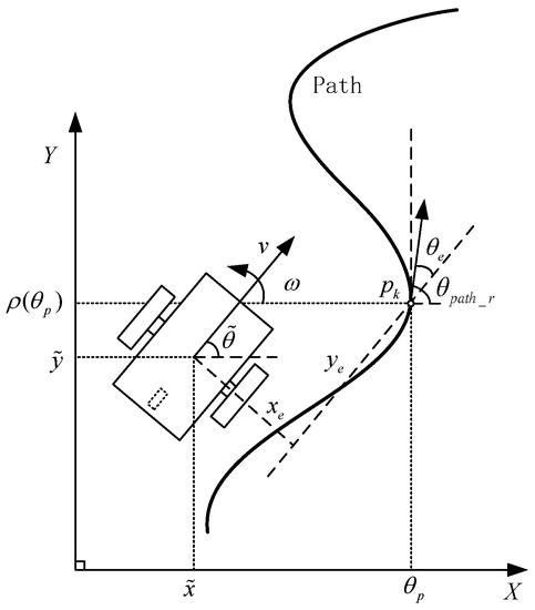
Figure 1.
Mobile robot path-following schematic.
2.2. Path-Following
As distinguished from the trajectory tracking problem, the path-following problem aims at moving the system along a geometric reference without any pre-specified timing information. It is assumed that the parametrized regular curve in the two-coordinate space [30] is as given in Equation (2).
Here, the scalar variable is called the path parameter, and Path: is a parametrization of Path. The geometric curve is satisfied with the characteristic of local bijectivity. The map p: is assumed to be sufficiently often continuously differentiable. As shown in Figure 1, the path with the coordinate points can be considered as , , where the time t of is set arbitrarily. The direction line can be virtually set as the tangent line of the path at the point. In this paper, the discrete coordinate point of the path is and the mobile robot’s desired position can be considered as the path with a time law [1].
The position error of the mobile robot for path-following can be expressed by the tracking error expression [29] in Equation (3).
The goal of path-following is to guarantee that the position error converges, i.e., .
3. Path-Following and Obstacle Avoidance Control Strategy Incorporating Reinforcement Learning
In this section a reinforcement learning method is used for the investigation of path-following and obstacle avoidance for nonholonomic wheeled mobile robots, based on the kinematic model and the path-following model in the above section.
3.1. Reinforcement Learning Control Method
RL can directly interact with the environment without having any information in advance [19]. Classical reinforcement learning approaches are based on the Markov decision process (MDP), consisting of the set of states S, the set of actions A, the rewards R, and the transition probabilities T that capture the dynamics of a system [31]. According to the Markov property, the next state is obtained by the model from the state and action . This is called transition probability model , and a reward is obtained after state transition evaluation. The whole process from to can be considered as one training step of the reinforcement learning, where the aim is to find the optimal strategy , i.e., the stochastic policy or the deterministic policy that can be evaluated by using the value function or the state value function , which is expressed as:
where both value functions are shown in Equations (5) and (6) separately, and the accumulated discounted reward is given in Equation (7).
Recently, researchers have used the techniques of experience replay and a separate target network to eliminate instability by establishing the large-scale neural network called DQN in the RL problem. This has already shown excellent performance [32]. However, the DQN is limited by the discrete nature of its action space, and is not capable of dealing with continuous control problems [19]. To overcome the difficulty of accurate expressions for actions, deterministic policy gradient (DPG) is proposed for handling the continuous action space [33]. The deterministic policy is considered instead of the policy selected stochastically in state S, and the vector is its parameter. If the target policy is deterministic, then the value function can be expressed as , and the expectation can be avoided [33] in Equation (8):
If there is an approximator parametrized by , then it can be optimized by minimizing the following loss:
where is dependent on :
can be considered as the critic, which is learned by Q-learning using the Bellman equation and is updated by the expected return from the actor network using a DPG [33]:
Regarding the approach to handling large networks in DQN, the DDPG algorithm uses experience replay and separate target network techniques to deal with large-scale neural network approximators in deep reinforcement learning. The DDPG has two basic networks called critic and actor, respectively. The whole process structure of the algorithm is presented in Figure 2 and will be used in the following study of the control strategy. The first step of the algorithm is that the actor network selects the action (control values), the corresponding reward, and the next state through the actor network, according to the training environment, and these are stored in the replay buffer with the action and state. Then, selecting a set consisting of state, action, forward, and updated state from the replay buffer, the target critic network selects the critic parameters according to the behavior selected by the target actor network. The critic network also gives other critic parameters, and then the network update of the critic network will be realized by the gradient of TD (temporal difference) errors with those parameters. Finally, the critic network selects the action and the current state according to the actor network, to realize the forward and backward propagation of the network. This process achieves the updating of the actor network by the policy gradient. For the updating of the networks, the critic network is updated using the gradient of the loss function in (9), whereas the actor network uses a deterministic policy gradient, which can be found in (11).
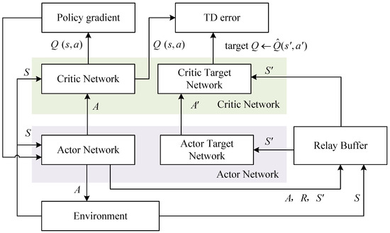
Figure 2.
Actor–critic architecture of path-following and obstacle avoidance control.
3.2. Path-Following and Obstacle Avoidance Controller Based on DDPG
The algorithm performance and convergence speed of reinforcement learning are highly dependent on the correctness of the state space, action space, and reward. In the process of path-following and obstacle avoidance control, the solution of using two agents to achieve control tasks is obviously complicated and inconvenient [19]. In order to solve these issues, this paper unifies the two types of control by designing the state space and reward based on the specific requirements of the two types of control. This can ensure that the wheeled mobile robot achieves effective obstacle avoidance in the process of path-following.
In this paper, the primary goal is to minimize the errors expressed in the above goal of path-following, and the state space S is expressed as:
Considering obstacle avoidance control, the state space S can be redesigned as:
where and are the parameters of state for avoiding collisions, represents the distance between the obstacle center and the center of the robot, and t is the current time step, as shown in Figure 3. When the robot is far from the obstacle during path-following, the current control of the robot is considered to be relatively safe. The parameter is only considered when the robot goes to the safe region setting for avoiding obstacles. Therefore, this paper also divides the obstacle avoidance region for the obstacle, as shown in Figure 3 and Figure 4, and the parameters and are defined as follows:
where is the radius of the minimum obstacle avoidance control area.
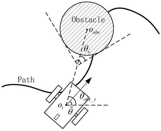
Figure 3.
Obstacle avoidance illustration for a NWMR for path-following.
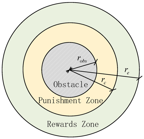
Figure 4.
Schematic diagram of the components of the obstacle avoidance region.
The above is considered for the case of a single obstacle; it is not applicable to an environment containing multiple obstacles. In the case of multiple obstacles, the minimum representative value technique is proposed, considering several and , where the minimum values for both parameters are chosen as the elements of state for avoiding more collisions. The minimum representative value can be expressed as:
where k is the number of obstacles. Since there are multiple obstacles corresponding to different states, for reward setting considering all obstacles, penalty rewards are considered for them all. The minimum representative approach is then able to ensure that the agent maintains the behavior of obstacle avoidance during training and that it is feasible to achieve path-following and obstacle avoidance control for NWMRs.
In RL, the agent can learn to adjust its strategy according to the reward so that it can avoid multiple obstacles in path-following. Compared with the environmental state set according to the number of obstacles [28], this method can reduce the dimensionality of the state, thus achieving the effect of obstacle avoidance while reducing the computational burden and saving computing resources.
Considering the path-following issue only, based on the current evaluation of the robot status, the basic reward function is designed as:
When the robot moves into obstacle avoidance regions, the reward function is redesigned by using extra punishments or rewards on the basis of the original reward for tracking control, making the robot capable of bypassing the obstacle without collisions. Based on the division into different regions, the reward function for obstacle avoidance regions is expressed as:
where and are parameters that limit the reward and penalty, respectively. Both are able to prevent large, abrupt changes in the single-step reward, which can cause instability during training. More specifically, not only is the distance to the circle of the obstacle for the reward function considered but the errors between the robot navigation angle and the obstacle direction are also taken into account in this work when the NWMR moves into the Punishment Zone. Based on this concept, the reward function is represented as:
where is the parameter that moderates the penalty according to the errors .
If the NWMR collides with an obstacle during movement, then the task is considered a failure, a severe penalty is imposed directly as the reward in this step, and the training environment will convert to a new episode. Due to this severe negative reward, the robot is able to follow the basic path-tracking control strategy in the learning of obstacle avoidance, and eventually it is able to complete the motion control for the whole set path while avoiding the obstacles.
According to the above path-following and obstacle avoidance control strategy, the control process based on deep reinforcement learning is shown in Algorithm 1:
| Algorithm 1 Path-Following and Obstacle Avoidance Control Strategy for NWMRs |
| Require: robot random initial pose , path p, training , time step , learning rate for actor network and for critic network, parameter for stability of training, discount factor , experience replay buffer size N, the number k of obstacles, obstacle avoidance position , parameters , , , , and parameters related to obstacle avoidance , , , , ; |
| Intialize: critic network and actor network randomly, target network and ; |
| 1: for each do |
| 2: Obtain an observation of random initial pose to NWMR in environment, then output position error through path parameters, and finally obtain initial state ; |
| 3: for all do |
| 4: Initialize a random noise for the deterministic strategy; |
| 5: Randomly select an action as a control input based on the current environment strategy and exploration noise ; |
| 6: Execute u, then obtain reward and new state ; |
| 7: Put into experience replay buffer D; |
| 8: if number of > Memory then |
| 9: Extract randomly a batch of transitions from D; |
| 10: Update actor network and critic network, (9) (11); |
| 11: Update target network for stable training as: |
| 12: |
| 13: |
| 14: end if |
| 15: end for |
| 16: end for |
4. Results and Discussions
In order to verify the path-following and obstacle avoidance control strategy proposed in this paper, several sets of simulation experiments were conducted. Firstly, only the path-following was investigated and compared with the model predictive control (MPC) method. Secondly, path-following and obstacle avoidance simulation experiments were conducted, and results were given for validating the effectiveness of the proposed controller performance for multiple obstacle avoidance in training environments.
4.1. Training Setting
In the environment of the simulation, the initial position of the NWMR was randomly selected around the end point of the path, where the initial position can be expressed as:
where were used to generate different initial values in each start episode in the environment, and the maximum linear and angular velocities were set as 3 m/s and rad/s, respectively, in the training. In the training simulation, the time step was set to 0.5 s (2 Hz) and the size of the mini-batch to 64. To establish the training networks, the Adam optimizer was used to train both the actor and critic networks. The hyperparameters are shown in Table 1, and the networks were built using the machine learning library . The learning rate was set to 0.001 for the actor network, and was set to 0.01 for the critic network. The target network transition gain was selected as 0.01, and the discount factor was selected as 0.9. For exploration of the training, the Ornstein–Uhlenbeck exploration method discussed in [34] was used.

Table 1.
Hyperparameters of networks.
The sinusoidal path can be parametrized, as investigated in [22], as:
4.2. Comparison of Path-Following between the Proposed Method and MPC
In this experiment, the agent was trained for 400 episodes, with a total of 240,000 training steps in the simulations. To validate the path-following capabilities of the proposed method, the MPC algorithm [35] was introduced to present its performance for path-following, and a comparison was made between the two methods. Moreover, the effectiveness of the proposed algorithm is further illustrated by showing the following effects at different training stages.
Figure 5a shows the path-following effect of the proposed algorithm and also adds the MPC algorithm for a comparison of the results. As shown in Figure 5b, errors for each waypoint of the path are presented, It is shown that the convergence performance of the proposed algorithm is better than that of the MPC algorithm at the turn. It can also be shown that the longitudinal error performance using the proposed algorithm is better than that using the MPC and that the other errors show the same or better performance. The comparison of inputs between the two algorithms is given in Figure 5c. Figure 5d presents the reward changes in every step of the final episode in the training, and Figure 5e shows the average score per 100 episodes in the whole training process. It can be shown that the trend of the reward score is consistent with the path-following effect, by combining the results in Table 2, which represents the four stages of the training process, chosen as 100, 200, 300, and 400 episodes. It can be shown that the agent tended to show worse performance results for following the path at the initial stage of the training, which is irrelevant to the initial purpose of path-following. As the training continued, the path-following performance tended to develop, resulting in a decrease in the cross-track error and the angular error, with scores climbing steadily. Finally, the proposed algorithm results in better performance than MPC considering the comparison of the longitudinal and cross errors.
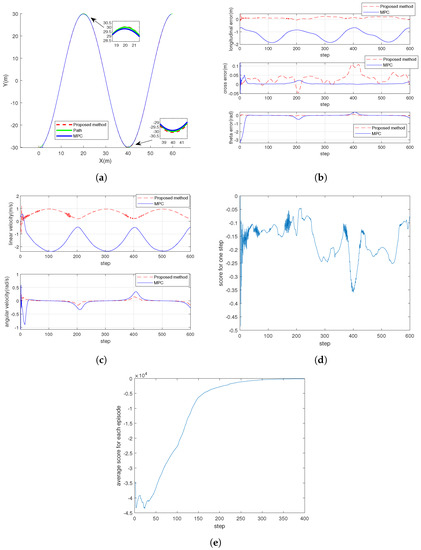
Figure 5.
Comparisons of proposed method and MPC for performance of path-following control. (a) Comparison of paths for following. (b) Errors in path-following. (c) Inputs for path-following. (d) Scoring of each step with proposed method. (e) Average scoring for each episode with proposed method.
Table 2.
Path-following controller performance at different training stages.
According to the results of the path-following simulation experiments, the proposed control strategy performs more robustly and has more accurate characteristics. It is capable of moving close to the waypoints of the path with different starting points, whereas the comparison algorithm needs to adjust its parameters to meet the requirements of the initial point.
4.3. The Performance of Path-Following with Collision Avoidance
In this experiment, the agent was trained for 1000 episodes, with a total of 600,000 training steps in the simulations. Two obstacles were chosen in order to perform a validation study of the proposed algorithm for path-following and obstacle avoidance. The learning rate was reduced to 0.002 for the critic network, and the discount factor was changed to 0.98. The number of obstacles k was set at two, with centers at [10, 0] and [47, −10] around the waypoints of the reference path, and the common parameters , , were set to 3.5 m, 5.5 m, and 7.5 m, respectively. The parameters and were set to 100 and 10, as scores for the reward and penalty, respectively. For each obstacle, the severe penalty was 100 in every episode, and the parameter was set at .
Figure 6a shows the results of the proposed algorithm when considering path-following and obstacle avoidance control simultaneously. In Figure 6b, the errors at each waypoint of the path are presented. The inputs of the proposed algorithms are given in Figure 6c. Figure 6d presents the reward changes in every step in final episode of the training. It can also be seen in Figure 6d that there is a certain penalty score when the robot moves to the obstacle avoidance area, which shows that the robot is able to achieve the obstacle avoidance operation from the divided area in the case of path-following. Figure 6e shows the reward changes in the final episode and in all episodes in the training, and it can be seen that the trend of the reward score is consistent with the path-following effect, by combining the results in Table 3, which represents the four stages of the training process, chosen as 100, 200, 400, and 1000 episodes.
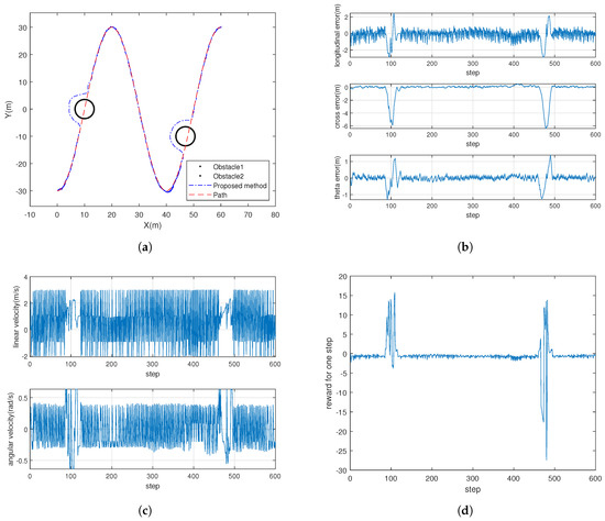
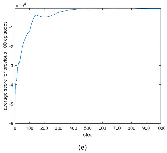
Figure 6.
Performances of the proposed method for path-following and obstacle avoidance control. (a) Comparison of paths for following. (b) Errors in path-following. (c) Inputs for path-following. (d) Scoring for each step with proposed method. (e) Average scoring for each episode with proposed method.
Table 3.
Path-following and obstacle avoidance controller performance at different training stages.
5. Conclusions
In this paper, a deep-reinforcement-learning-based controller was proposed for path-following for nonholonomic wheeled mobile robots(NWMRs). The deep deterministic policy gradient (DDPG) algorithm was utilized to establish a control law for linear and steering velocities, and the learning-based control policy was trained using repeated path-following simulations. The path-following results demonstrated the effectiveness of the proposed method, and the comparisons showed that our method had better efficiency and more robust performance than the MPC method for path-following control without collisions. For research on path-following and obstacle avoidance control, a new approach was proposed to deal with redesigning the state and reward in RL. Moreover, minimum value techniques for the state were given for the path-following and obstacle avoidance controller, and the results showed the feasibility of solving the multiple obstacles environment problem during path-following for the control of NWMRs.
Author Contributions
Conceptualization, X.C. and S.Z.; methodology, S.Z.; software, S.Z.; validation, X.C., S.C. and J.Z.; formal analysis, S.C. and J.Z.; investigation, X.C. and S.Z.; resources, X.C.; data curation, S.Z.; writing—original draft preparation, S.Z.; writing—review and editing, X.C.; visualization, S.Z.; supervision, Q.X.; project administration, Q.X.; funding acquisition, X.C. All authors have read and agreed to the published version of the manuscript.
Funding
This research was funded by the Key-Area Research and Development Program of Guangdong Province, grant number 2019B090918004.
Institutional Review Board Statement
Not applicable.
Informed Consent Statement
Not applicable.
Data Availability Statement
Not applicable.
Conflicts of Interest
The authors declare no conflict of interest.
Abbreviations
The following abbreviations are used in this manuscript:
| NWMR | Nonholonomic Wheeled Mobile Robot |
| RL | Reinforcement Learning |
| DDPG | Deep Deterministic Policy Gradient |
| DPG | Deterministic Policy Gradient |
| DQN | Deep Q-Network |
| SCDRL | Smoothly Convergent Deep Reinforcement Learning |
| MPC | Model Predictive Control |
| GVF | Guiding Vector Field |
| SMC | Sliding Mode Control |
| PID | Proportional Integral Derivative |
| MDP | Markov Decision Process |
References
- Faulwasser, T.; Kern, B.; Findeisen, R. Model predictive path-following for constrained nonlinear systems. In Proceedings of the 48h IEEE Conference on Decision and Control (CDC) Held Jointly with 2009 28th Chinese Control Conference, Shanghai, China, 15–18 December 2009; pp. 8642–8647. [Google Scholar]
- Sun, Z.; Xie, H.; Zheng, J.; Man, Z.; He, D. Path-following control of Mecanum-wheels omnidirectional mobile robots using nonsingular terminal sliding mode. Mech. Syst. Signal Process. 2021, 147, 107128. [Google Scholar] [CrossRef]
- Chen, J.; Wu, C.; Yu, G.; Narang, D.; Wang, Y. Path Following of Wheeled Mobile Robots Using Online-Optimization-Based Guidance Vector Field. IEEE/ASME Trans. Mechatron. 2021, 26, 1737–1744. [Google Scholar] [CrossRef]
- Wang, H.; Tian, Y.; Xu, H. Neural adaptive command filtered control for cooperative path following of multiple underactuated autonomous underwater vehicles along one path. IEEE Trans. Syst. Man Cybern. Syst. 2021, 52, 2966–2978. [Google Scholar] [CrossRef]
- Liang, X.; Qu, X.; Hou, Y.; Li, Y.; Zhang, R. Finite-time unknown observer based coordinated path-following control of unmanned underwater vehicles. J. Frankl. Inst. 2021, 358, 2703–2721. [Google Scholar] [CrossRef]
- Rubí, B.; Morcego, B.; Pérez, R. Deep reinforcement learning for quadrotor path following with adaptive velocity. Auton. Robot. 2021, 45, 119–134. [Google Scholar] [CrossRef]
- Eskandarpour, A.; Sharf, I. A constrained error-based MPC for path following of quadrotor with stability analysis. Nonlinear Dyn. 2020, 99, 899–918. [Google Scholar] [CrossRef]
- Kapitanyuk, Y.A.; Proskurnikov, A.V.; Cao, M. A guiding vector-field algorithm for path-following control of nonholonomic mobile robots. IEEE Trans. Control. Syst. Technol. 2017, 26, 1372–1385. [Google Scholar] [CrossRef] [Green Version]
- Napolitano, O.; Fontanelli, D.; Pallottino, L.; Salaris, P. Information-Aware Lyapunov-Based MPC in a Feedback-Feedforward Control Strategy for Autonomous Robots. IEEE Robot. Autom. Lett. 2022, 7, 4765–4772. [Google Scholar] [CrossRef]
- Subari, M.A.; Hudha, K.; Kadir, Z.A.; Dardin, S.M.F.S.M.; Amer, N.H. Path following control of tracked vehicle using modified sup controller optimized with particle swarm optimization (PSO). Int. J. Dyn. Control. 2022, 1–10. [Google Scholar] [CrossRef]
- Rukmana, M.A.F.; Widyotriatmo, A.; Siregar, P.I. Anti-Jackknife Autonomous Truck Trailer for Path Following Control Using Genetic Algorithm. In Proceedings of the 2021 International Conference on Instrumentation, Control, and Automation (ICA), Bandung, Indonesia, 25–27 August 2021; pp. 186–191. [Google Scholar]
- Nguyen, A.T.; Sentouh, C.; Zhang, H.; Popieul, J.C. Fuzzy static output feedback control for path following of autonomous vehicles with transient performance improvements. IEEE Trans. Intell. Transp. Syst. 2019, 21, 3069–3079. [Google Scholar] [CrossRef]
- Martinsen, A.B.; Lekkas, A.M. Curved path following with deep reinforcement learning: Results from three vessel models. In Proceedings of the OCEANS 2018 MTS/IEEE Charleston, Charleston, SC, USA, 22–25 October 2018; pp. 1–8. [Google Scholar]
- Szepesvári, C. Algorithms for reinforcement learning. Synth. Lect. Artif. Intell. Mach. Learn. 2010, 4, 1–103. [Google Scholar]
- Duan, K.; Fong, S.; Chen, C.P. Reinforcement learning based model-free optimized trajectory tracking strategy design for an AUV. Neurocomputing 2022, 469, 289–297. [Google Scholar] [CrossRef]
- Cao, S.; Sun, L.; Jiang, J.; Zuo, Z. Reinforcement Learning-Based Fixed-Time Trajectory Tracking Control for Uncertain Robotic Manipulators with Input Saturation. IEEE Trans. Neural Netw. Learn. Syst. 2021. [Google Scholar] [CrossRef] [PubMed]
- Okafor, E.; Udekwe, D.; Ibrahim, Y.; Bashir Mu’azu, M.; Okafor, E.G. Heuristic and deep reinforcement learning-based PID control of trajectory tracking in a ball-and-plate system. J. Inf. Telecommun. 2021, 5, 179–196. [Google Scholar] [CrossRef]
- Wang, S.; Yin, X.; Li, P.; Zhang, M.; Wang, X. Trajectory tracking control for mobile robots using reinforcement learning and PID. Iran. J. Sci. Technol. Trans. Electr. Eng. 2020, 44, 1059–1068. [Google Scholar] [CrossRef]
- Woo, J.; Yu, C.; Kim, N. Deep reinforcement learning-based controller for path following of an unmanned surface vehicle. Ocean. Eng. 2019, 183, 155–166. [Google Scholar] [CrossRef]
- Nie, C.; Zheng, Z.; Zhu, M. Three-dimensional path-following control of a robotic airship with reinforcement learning. Int. J. Aerosp. Eng. 2019, 2019, 7854173. [Google Scholar] [CrossRef]
- Liu, M.; Zhao, F.; Yin, J.; Niu, J.; Liu, Y. Reinforcement-Tracking: An Effective Trajectory Tracking and Navigation Method for Autonomous Urban Driving. IEEE Trans. Intell. Transp. Syst. 2021. [Google Scholar] [CrossRef]
- Zhao, Y.; Qi, X.; Ma, Y.; Li, Z.; Malekian, R.; Sotelo, M.A. Path following optimization for an underactuated USV using smoothly-convergent deep reinforcement learning. IEEE Trans. Intell. Transp. Syst. 2020, 22, 6208–6220. [Google Scholar] [CrossRef]
- Wang, Y.; Sun, J.; He, H.; Sun, C. Deterministic policy gradient with integral compensator for robust quadrotor control. IEEE Trans. Syst. Man Cybern. Syst. 2019, 50, 3713–3725. [Google Scholar] [CrossRef]
- Zhu, W.; Guo, X.; Fang, Y.; Zhang, X. A path-integral-based reinforcement learning algorithm for path following of an autoassembly mobile robot. IEEE Trans. Neural Netw. Learn. Syst. 2019, 31, 4487–4499. [Google Scholar] [CrossRef]
- Chen, L.; Chen, Y.; Yao, X.; Shan, Y.; Chen, L. An adaptive path tracking controller based on reinforcement learning with urban driving application. In Proceedings of the 2019 IEEE Intelligent Vehicles Symposium (IV), Paris, France, 9–12 June 2019; pp. 2411–2416. [Google Scholar]
- Lapierre, L.; Zapata, R.; Lepinay, P. Combined path-following and obstacle avoidance control of a wheeled robot. Int. J. Robot. Res. 2007, 26, 361–375. [Google Scholar] [CrossRef]
- Meyer, E.; Robinson, H.; Rasheed, A.; San, O. Taming an autonomous surface vehicle for path following and collision avoidance using deep reinforcement learning. IEEE Access 2020, 8, 41466–41481. [Google Scholar] [CrossRef]
- Rubí, B.; Morcego, B.; Pérez, R. Quadrotor Path Following and Reactive Obstacle Avoidance with Deep Reinforcement Learning. J. Intell. Robot. Syst. 2021, 103, 1–17. [Google Scholar] [CrossRef]
- Kanayama, Y.; Kimura, Y.; Miyazaki, F.; Noguchi, T. A stable tracking control method for an autonomous mobile robot. In Proceedings of the IEEE International Conference on Robotics and Automation (ICRA), Cincinnati, OH, USA, 13–18 May 1990; pp. 384–389. [Google Scholar]
- Faulwasser, T.; Findeisen, R. Nonlinear model predictive control for constrained output path following. IEEE Trans. Autom. Control. 2015, 61, 1026–1039. [Google Scholar] [CrossRef] [Green Version]
- Sutton, R.S.; Barto, A.G. Reinforcement Learning: An Introduction; MIT Press: Cambridge, MA, USA, 2018. [Google Scholar]
- Mnih, V.; Kavukcuoglu, K.; Silver, D.; Rusu, A.A.; Veness, J.; Bellemare, M.G.; Graves, A.; Riedmiller, M.; Fidjeland, A.K.; Ostrovski, G.; et al. Human-level control through deep reinforcement learning. Nature 2015, 518, 529–533. [Google Scholar] [CrossRef]
- Silver, D.; Lever, G.; Heess, N.; Degris, T.; Wierstra, D.; Riedmiller, M. Deterministic policy gradient algorithms. In Proceedings of the International Conference on Machine Learning, PMLR, Bejing, China, 22–24 June 2014; pp. 387–395. [Google Scholar]
- Lillicrap, T.P.; Hunt, J.J.; Pritzel, A.; Heess, N.; Erez, T.; Tassa, Y.; Silver, D.; Wierstra, D. Continuous control with deep reinforcement learning. arXiv 2015, arXiv:1509.02971. [Google Scholar]
- Zhang, J.J.; Fang, Z.L.; Zhang, Z.Q.; Gao, R.Z.; Zhang, S.B. Trajectory Tracking Control of Nonholonomic Wheeled Mobile Robots Using Model Predictive Control Subjected to Lyapunov-based Input Constraints. Int. J. Control. Autom. Syst. 2022, 20, 1640–1651. [Google Scholar] [CrossRef]
Publisher’s Note: MDPI stays neutral with regard to jurisdictional claims in published maps and institutional affiliations. |
© 2022 by the authors. Licensee MDPI, Basel, Switzerland. This article is an open access article distributed under the terms and conditions of the Creative Commons Attribution (CC BY) license (https://creativecommons.org/licenses/by/4.0/).