Application of Machine Learning Tools for Long-Term Diagnostic Feature Data Segmentation

Abstract

In this paper, a novel method for long-term data segmentation in the context of machine health prognosis is presented. The purpose of the method is to find borders between three data segments. It is assumed that each segment contains the data that represent different statistical properties, that is, a different model. It is proposed to use a moving window approach, statistical parametrization of the data in the window, and simple clustering techniques. Moreover, it is found that features are highly correlated, so principal component analysis is exploited. We find that the probability density function of the first principal component may be sufficient to find borders between classes. We consider two cases of data distributions, Gaussian and $\alpha$-stable, belonging to the class of non-Gaussian heavy-tailed distributions. It is shown that for random components with Gaussian distribution, the proposed methodology is very effective, while for the non-Gaussian case, both features and the concept of moving window should be re-considered. Finally, the procedure is tested for real data sets. The results provided here may be helpful in understanding some specific cases of machine health prognosis in the presence of non-Gaussian noise. The proposed approach is model free, and thus it is universal. The methodology can be applied for any long-term data where segmentation is crucial for the data processing.

1. Introduction

Condition monitoring systems are designed to collect a massive amount of data during the operation of machines. The purpose of this is to assess the condition of the machine. Typically, there is a set of features extracted from raw signals, and each of features is compared to so-called limit values (threshold corresponding to change from “Good Condition” to “Warning” and “Warning” to “Alarm”). In some cases, such limit values are provided by the manufacturer. Unfortunately, in many cases, especially when the machine is pretty unique, we do not know about the limit values or expected lifetime.

In the paper, we propose an approach that based on historical data may identify the border of classes good condition/warning/alarm, i.e., identify the points in the data when the machine changes the condition. The change in condition is manifested by the change in statistical properties of the collected data. There are many models of the lifetime curve. Here, we follow the shape of the curve that consists of three regimes. In the first regime, there is a nearly constant value of feature with some small variation. Next, in regime two, there is linear growth also, and the variation of random components is smoothly growth. Finally, in regime three, the feature is exponentially increasing, and the random component has significant variation. Figure 1 presents the conceptual model of the input data.

The data describing the degradation of the machine are not purely deterministic and they contain some randomness. In this paper, we assume two cases. In the first one, the random component follows the Gaussian distribution and, as mentioned, its variance is constant in the first segment, linearly increasing over time in the second segment and finally exponentially increasing in the third segment.

In the second case, the character of the noise is non-Gaussian, and we assume it can be modeled by $\alpha$-stable distribution with $\alpha <2$. Moreover, the scale parameter $\sigma$ is changing over time (it corresponds to variance for Gaussian distribution).

As the raw data are a random, non-stationary process, we propose to use moving window with fixed size for primary segmentation, then we describe the data in each segment by simple statistical descriptors (sample mean, sample variance, sample kurtosis, etc.). Obviously, such features are highly redundant, especially when there is many of them; thus the basic technique for dimensionality reduction is applied. Finally, the reduced data set is clustered by various machine learning algorithms, and the most efficient scenario is selected. Such an approach is quite simple and effective for the Gaussian distribution case. Unfortunately, for the non-Gaussian case, both statistical parameters as well as clustering techniques must be deeply revised, as $\alpha$-stable distributed data contain many outliers. In the paper, we propose a methodology for finding the limit values for the mentioned classes (good condition/warning/alarm), and we illustrate the efficiency of approach for simulated and real data. We explain that the source of relatively poor efficiency may be related to a non-Gaussian distribution of random components, and we highlight that robust methods for parameterization and clustering are needed.

2. State of the Art

There is a lot of data collected every minute in various branches of the economy, such as industry, financial sector and many others. Data regarding currency exchange [1], stock exchange, raw materials prices [2,3], energy consumption/prices [4,5], etc., are collected, processed and analyzed to understand the nature of important phenomena. However, each case is specific and requires appropriate methodology for data analysis. In this paper, we focus on long-term data from condition monitoring (CM) systems; however, some inspirations from other areas are also helpful.

Nowadays, the condition monitoring systems are frequently used to monitor current state of the given machine. Although there are at least several freely-available data sets, there are just a few practical examples of how to process and analyze long-term data acquired in industrial installations. There are many papers on data modeling for prognosis, but these works seem to be more theoretical (data sets from test rigs, accelerated fatigue tests with artificially initiated fault, etc.) than really applied to the actual industrial systems with natural degradation processes.

Just to mention several practical implementations, one may focus on [6] where the procedure of load-dependent features processing with application to wind turbine bearings was proposed. Another example proposed by Ignasiak et al. [7] discussed a comparative study on statistical and energy-based parameters analysis in a long-term context, also for a wind turbine. Wodecki et al. [8] analyzed the overheating problem for heavy-duty machines operating in the underground mine. Their method focused on temperature change detection in the long-term data set using Anderson–Darling statistics. Grzesiek et al. [9] proposed a statistical test for anomaly detection in long-term temperature data analysis for gearbox diagnostics used in underground mine. Wang et al. [10] introduced a hybrid prognostics method for estimating the remaining useful life of wind turbine bearings. Li et al. [11] developed an approach for predicting for a lithium-ion battery under vibration stress using the Elman neural network.

Analysis of the non-stationary data using moving window is commonly used to investigate local properties of the data, and was used, among others, by Staszewski et al. (moving window and kurtosis estimation in raw vibration for local damage detection) [12] or Zimroz et al. (moving window for HI from wind turbine condition monitoring system to estimate regression between health index (HI) and operational parameters) [6].

It was also shown that window selection is critical in forecasting [13]. In signal processing, the window length selection was clearly discussed in [14], where short time Fourier transform (STFT) was proposed to analyze non-stationary data. Haoran Yan et al. [15] introduced a methodology based on long short-term memory for predicting gear remaining useful life (RUL). As mentioned, simple statistics such as sample mean, sample variance, sample kurtosis, etc., are often used in condition monitoring for signal parameterization. In this paper, it is proposed to use such statistical descriptors in order to differentiate segments from different regimes. Initially, several statistics with theoretical potential in considered context are proposed. Finally, the mean value, standard deviation (STD) and root mean square (RMS) are applied for each segment. Machine learning is frequently used for long-term data analysis for classification, detection, prognosis, etc., [16,17,18,19,20,21,22,23,24,25,26,27]. In this case, unsupervised classification, i.e., clustering, is required because every machine works in different conditions, and labeling data is not an easy task. Hence, the clustering approach has massive potential for dividing long-term data into several regimes. The authors of [17] proposed the long short-term memory (LSTM) network with the clustering method for multi-stage predicting RUL. Jaskaran Singh et al. [18] introduced an adaptive data-driven model-based approach to detecting regime-changing point by using K-means clustering. Additionally, there are a lot of applications for regime changing point detection in time series in different areas, such as financial data analysis, etc. [28,29,30,31,32,33,34,35,36,37,38]. Detection of change in time series is a very widely investigated problem.

Signal segmentation is frequently used in various signal processing applications to divide original data into homogeneous segments or to extract the pattern, etc. Kucharczyk et al. [39] used stochastic modeling for seismic signal segmentation. Gasior et al. [40] used segmentation for shock extraction in a sieving screen vibrations. A challenge in signal segmentation is when the difference between regimes is not so clear. One may say that regime A is smoothly transforming to regime B. This issue was investigated by Grzesiek et al. [41]. It is also the case here, especially as there is “no jump” from good condition to warning state, that the machine in good condition slowly starts the degradation process. Another issue is multiple change points and unit heterogeneity [42].

3. Problem Formulation

The prognosis in predictive maintenance is related to the forecasting of HI values for future time instances or estimation of a RUL time [43,44,45,46,47,48]. In any case, to deal with prediction, one needs a model of the degradation of the machine. It is the most frequent case that advanced mathematical models or machine learning (ML) approaches are used for prognosis. ML approach requires historical data to train the prediction system or establish a data-driven model for the prognosis. From the reliability theory, one may notice that there are several “general” degradation models. As mentioned, in this paper, we follow the idea that machine lifetime consists of three phases (see Figure 1):

(a)

Good condition, where HI is nearly constant (no degradation);

(b)

Slow degradation (HI is increasing slowly and approximately linearly);

(c)

Fast degradation (HI is rapidly growing like exponential function).

In such a case, the model of the degradation, in fact, consists of three sub-models (three regimes). It means that before the identification of the model, the data need to be segmented. Segments corresponding to given sub-models should be extracted, and the data in each segment should be modeled separately. Thus, for long-term data from the condition monitoring system, one needs to apply the segmentation procedure before modeling. In other words, one needs to find so called regime change points, where the data are changing their nature in the sense of statistical properties. In this paper, the general idea is to analyze locally statistical parameters by the moving window approach. For a priori selected window length and overlapping, simple descriptive statistics are calculated, and then these features for each segment are subjected to clustering. There are some challenging issues to solve. They are related to the segment size, overlapping, statistical parameters selection (features), and the clustering method. According to some earlier work and our experience, it may be necessary to use the further processing of features. In the next section, an original methodology to segment historical data from condition monitoring system is presented in detail.

In the case of non-Gaussian noise, many theoretical assumptions cannot be fulfilled, so a number of techniques cannot be applied. This happens because the high content of outliers in the data negatively affects the calculation of many statistics, especially the ones related to variance.

4. Methodology

The general idea of the methodology is presented in Figure 2. It is assumed that the historical data set from condition monitoring systems contains three regimes that follow the model discussed in [49,50]. The degradation model consists of deterministic and random parts. Using a moving window, one may consider the original data in the window as independent and identically distributed (i.i.d.) observations, so simple statistical descriptors can be used to characterize their local properties. To increase resolution in the time domain, one may use overlapping. It may be helpful to precisely detect the regime change point.

In many papers, it is shown that simple statistics are easy to use and may provide important information; however, they are usually correlated, so dimensionality reduction is recommended. By the appropriate transformation of extracted features, one may reduce the number of novel features and still preserve original information. It is proposed to use principal component analysis (PCA) here. In general, the PCA is used to reduce highly dimensional data to a data set of a lower size [51]. However, in some applications, the PCA is used to visualize reduced features in 2D or 3D space, so projection is into PC1-PC2 or PC1-PC3 space. We will follow this idea here as well to visualize the distribution of data in PC space and to understand the results of clustering. To find these three regimes, we use extracted features and several most popular algorithms for clustering implemented in the Matlab environment.

In the case of really high correlation in input data space, it may happen that PC1 contains almost all information. Then, for 1D time series (PC1 corresponds to input data acquired in time), simple probability density function estimation may be enough to find threshold values that will be able to divide the input data into three regimes. The final step of the procedure is related to the validation of clustering. We present the results of clustering using different colors applied to time series. In Figure 3, more detailed explanation regarding moving window and statistical parameter extraction is presented.

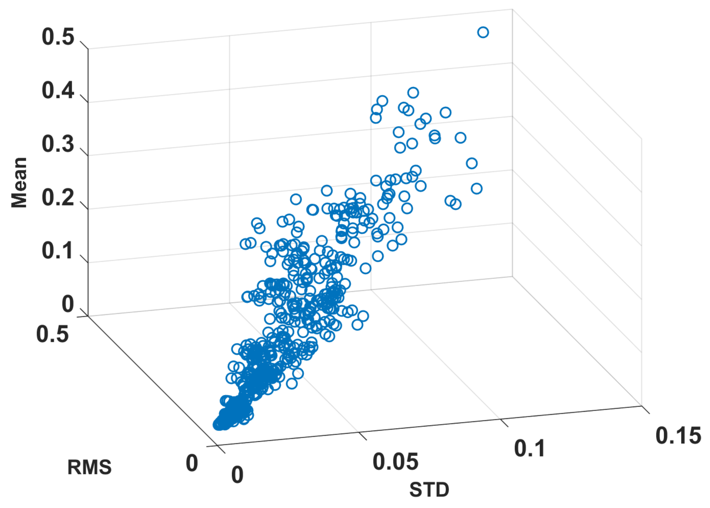
4.1. Segmentation and Descriptive Statistics Used as Features

In the parametrization, we calculate the appropriate statistics calculated for the data from the moving window with size w and overlapping o. The window size cannot be too small because the parameters extracted for a small data set will be very sensitive to any outliers or even small variations. From the other hand, it cannot be large, as the resolution in the time domain will be poor and the precision of the regime change detection will be limited. The parameters w = 50 [samples] and o = 80 [percent] are selected experimentally. For each segment, a set of statistical parameters is calculated. There are many statistical features that can be extracted from time series based on the proposed methodology. In this paper, initially seven popular parameters are tested (maximum, sample median, sample mean, sample standard deviation (STD), sample kurtosis, sample skewness, and root mean square (RMS) of the data) and used as the main features. However, after some preliminary analysis, only three of them are selected. This issue is discussed in the next parts.

The mathematical formulations of the used statistics are presented in

Table 1. Time domain features.

Feature	Formula
Max value	M = max($x_i$)
Sample median	$\left\{\begin{array}{c}{x}_{(n+1)/2},n\%2=1,\hfill \\ \frac{x_{(n/2)}+x_{(n/2)+1}}{2},n\%2=0,\hfill \end{array}\right.$
Sample mean value	$\overline{x}=\frac{1}{N}{\displaystyle \sum _{i=1}^N}{x}_i$
Sample standard deviation (STD)	$\widehat{\sigma }=\sqrt{\frac{1}{N-1}{\displaystyle \sum _{n=1}^N}{(x_i-\overline{x})}^2}$
Sample kurtosis	$\mathrm{K}=\frac{1}{N}{\displaystyle \sum _{i=1}^N}\frac{{(x_i-\overline{x})}^4}{{\widehat{\sigma }}^4}$
Sample skewness	$\mathrm{Sk}=\frac{1}{N}{\displaystyle \sum _{i=1}^N}\frac{{(x_i-\overline{x})}^3}{{\widehat{\sigma }}^3}$
root mean square	$\mathrm{RMS}=\sqrt{\frac{1}{N}{\displaystyle \sum _{i=1}^N}{x}_i^2}$

Where the symbol % indicates the modulo division, and the result is a remainder.

, where $x_1,x_2,\dots ,x_N$ is the analyzed sample and N is the total number of observations.

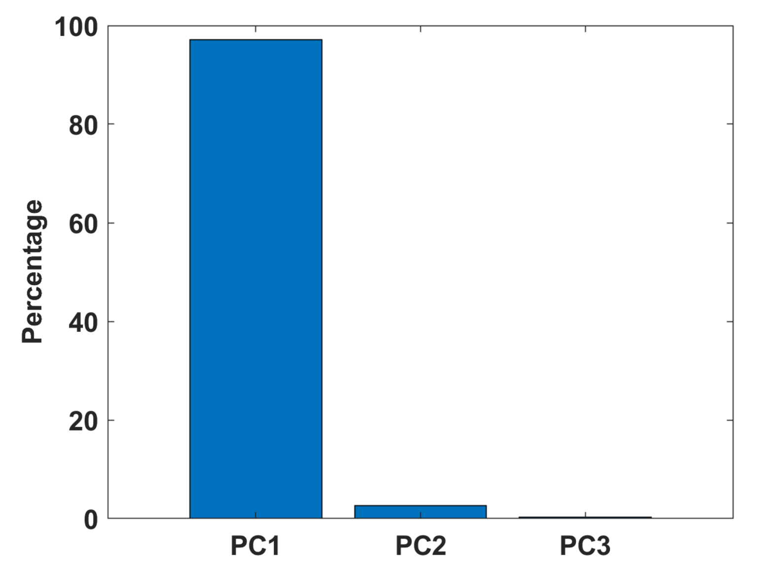
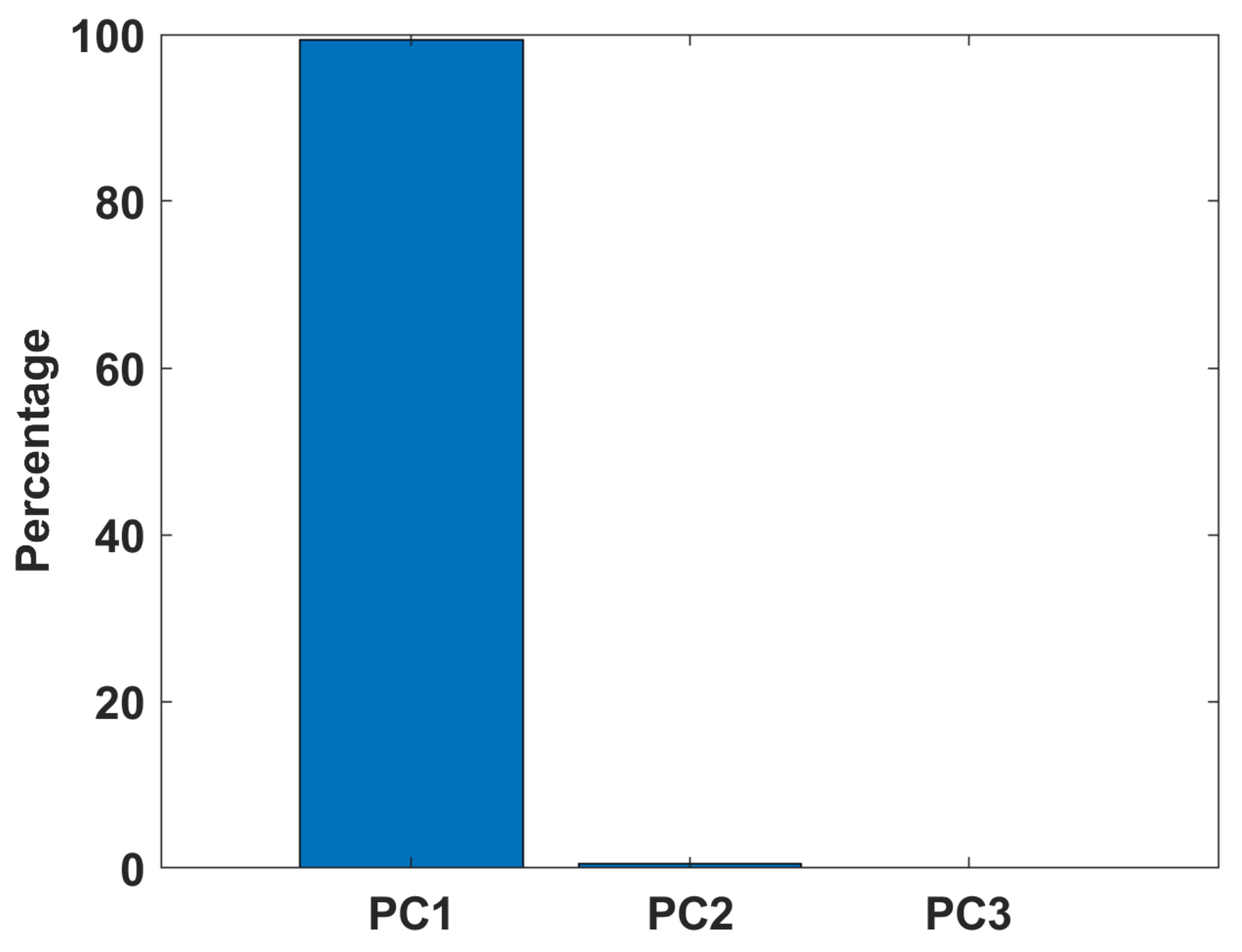
4.2. Principal Component Analysis

Principal component analysis (PCA) in the mathematical definition [51] is an orthogonal linear transformation that takes data to a new coordinate system. Assuming that a given multidimensional data set is arranged as N samples with M variables, it can be expressed as a point cloud in M-dimensional space. The aim of PCA is to translate the location and orientation of the new coordinate system so that the variance is maximized along the new dimensions. It is performed in a way that the most significant variance of the data is on the first coordinate axis, and the second-largest variance is on the second coordinate axis, and so on. The idea is visualized in Figure 4.

Principal component analysis can reduce the data dimension, thus preserving the components of the data set that have the most significant effect on variance. For example, Figure 4 presents that the first principal component (the longer arrow) describes most of the variance in the data. Hence, if one extracts only the coordinates projected on this axis, one would obtain a majority of information described by the entire data set (or rather the percentage of the information corresponding to the relative content of the variance described by this new dimension).

By utilizing the singular value decomposition (SVD), the principal components can be calculated based on N observations of M-dimensional data stacked into a matrix $X\in {\mathbb{R}}^{N\times M}$

$$\frac{1}{\sqrt{N-1}}\mathbf{X}=\mathbf{U}\mathsf{\Sigma }{\mathbf{V}}^T,$$

(1)

where $U\in {\mathbb{R}}^{N\times N}$ and $V\in {\mathbb{R}}^{M\times M}$ are unitary matrices and $\mathsf{\Sigma }\in {\mathbb{R}}^{N\times M}$ contains the nonnegative real singular values of non-increasing magnitude (${\sigma }_{pc1}\ge {\sigma }_{pc2}\ge \cdots \ge {\sigma }_{pcM}\ge 0$). Principal components are the orthonormal column vectors of the matrix V, and the variance of the i-th component is equal to ${\sigma }_{pci}^2$.

4.3. Kernel Density Estimation

The probability distribution function (pdf) can be estimated using the kernel density estimator [53,54]. For argument x, the estimated density is given by

$${\widehat{f}}_h\left(x\right)=\frac{1}{Nh}\sum _{i=1}^{N}W\left(\frac{x-x_i}{h}\right),$$

(2)

where $x_1,x_2,\dots ,x_N$ are observations, $W(·)$ is the kernel smoothing function, N is the sample size, and h is the bandwidth. In this paper, a Gaussian kernel is used. The Gaussian kernel is the most common one used in various applications. It corresponds to the Gaussian probability density function; however, it is also used to estimate the probability density functions from other distributions. The Gaussian kernel has the properties of having no overshoot to a step function input while minimizing the rise and fall time. The value of the bandwidth is obtained using the so-called Silverman’s rule of thumb [54]. For the Gaussian kernel, the optimal choice for h (that is, the bandwidth that minimizes the mean integrated squared error) is

$$h={\left(\frac{4{\widehat{\sigma }}^5}{3N}\right)}^{\frac{1}{5}}\approx 1.06\widehat{\sigma }{N}^{-1/5},$$

(3)

where $\widehat{\sigma }$ is the sample standard deviation and N is the number of observations.

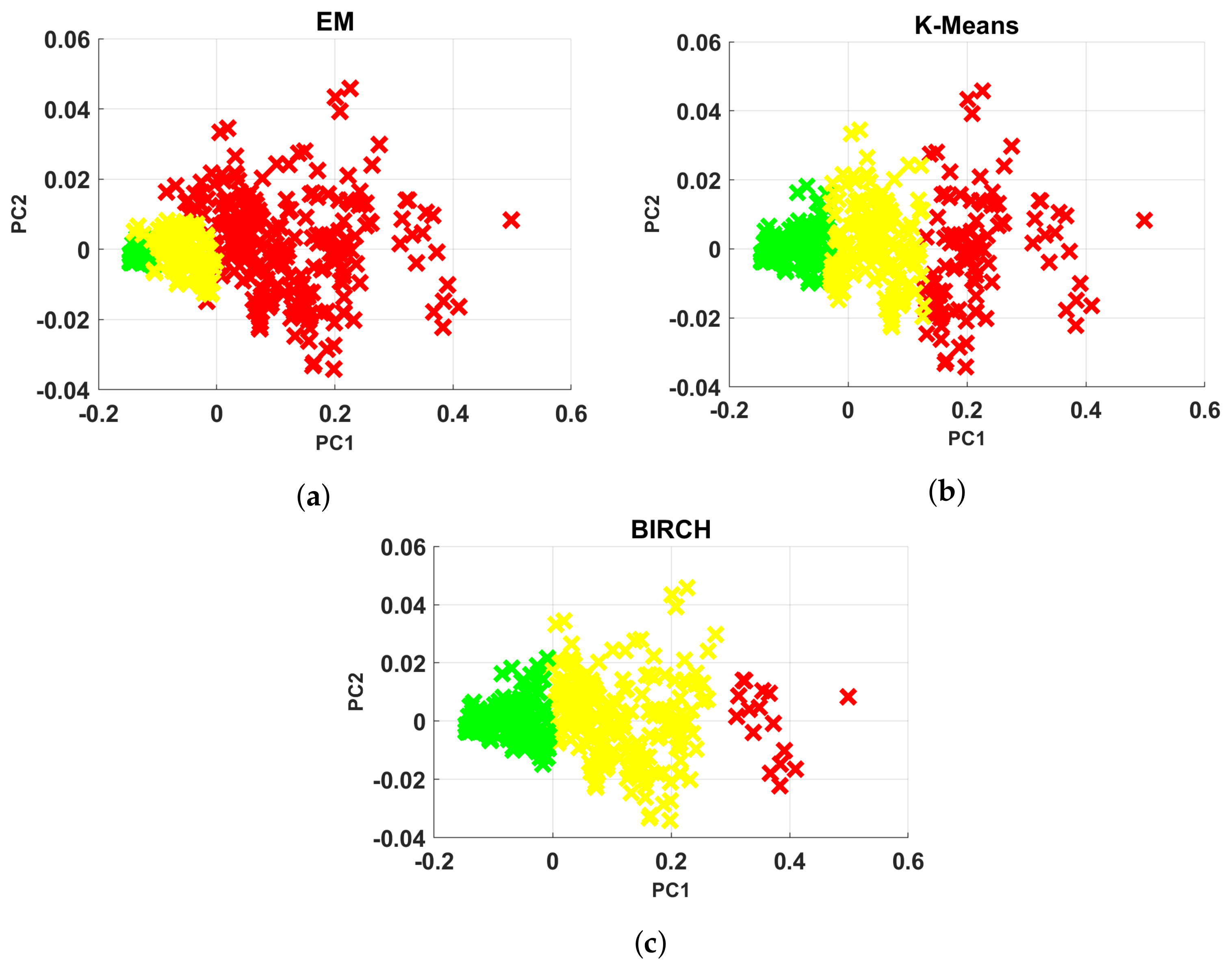
4.4. Cluster Analysis Techniques

In cluster analysis, many various algorithms are available that are characterized with different principles of operation and suitable for different scenarios. We test several popular methods using implementations prepared for Matlab. Finally, we have decided to use three algorithms providing the most promising results. Here, we recall three of the most suitable in our context.

• K-means clustering is a method of vector quantification that is originally derived from signal processing, and it is famous approach for clustering in data mining [55,56,57,58]. K-means clustering is used to decompose the n observations into k clusters whose observations belong to a cluster with its closest mean. According to the set of observations $x_1,x_2,\dots ,x_N$ where each observation is a M dimension vector. The target of K-means clustering is to divide N observation to $k<=N$ collection $S=(S_1,S_2,\dots ,S_k)$ such that the sum of the squares of the difference from the mean (i.e., variance) is minimized for each cluster.
• BIRCH (balanced iterative reducing and clustering using hierarchies) is one of the fastest clustering algorithms, introduced in refs. [59,60,61]. The main advantage of BIRCH is that it clusters incrementally and dynamically, attempting to produce the best quality given the time and memory constraints, with the requirement of only a single scan of the data set. However, it needs to specify the cluster count as an input variable. Additionally, BIRCH clustering is used in engineering applications. Lu et al. [62] introduced automatic fault detection based on BIRCH.
• Gaussian mixture modeling (GMM) is one of the popular methods used for unbalanced data clustering. The GMM is a probabilistic model that is based on the assumption that M-dimensional data X are arranged as a number of spatially-distributed Gaussian distribution modes with unknown parameters $\mu$ (list of M-dimensional means) and $\mathsf{\Sigma }$ (list of $M\times M$ covariance matrices).
  The expectation–maximization (EM) algorithm is used to estimate the parameters of GMM, thus allowing to cluster the data [63,64,65,66,67,68]. This method can be divided into two parts. At first, the expectation step (E-step) is used to estimate the probabilities for every point to be assigned to every cluster. Then the maximization step (M-step) is utilized to estimate the distributions based on the probabilities from E-step. Those two steps are iterated for a given number of iterations or until convergence.

5. Simulated Data Analysis

In this section, we apply the proposed procedure to simulated data. There are two cases: deterministic trend describing the degradation process mixed with (a) Gaussian and (b) non-Gaussian noise. The model is described as follows:

$$HI\left(t\right)=\left\{\begin{array}{c}a\hfill \\ b·t\hfill \\ c·\exp (d·t)\hfill \end{array}\right.\left.\begin{array}{c}t\le 1000\hfill \\ 1000<t\le 1600\hfill \\ t>1600\hfill \end{array}\right\}+\left\{\begin{array}{c}{\sigma }_1·N\left(t\right)\hfill \\ {\sigma }_2·t·N\left(t\right)\hfill \\ {\sigma }_3·\exp \left(t\right)·N\left(t\right)\hfill \end{array}\right.\left.\begin{array}{c}t\le 1000\hfill \\ 1000<t\le 1600\hfill \\ t>1600\hfill \end{array}\right\},$$

(4)

where $a,b,c,d$ are constant parameters that are related to deterministic parts, and ${\sigma }_1,{\sigma }_2,{\sigma }_3$ are parameters responsible for the scales of noise parts. Moreover, $\left\{N\right(t\left)\right\}$ is a noise.

Internal and external Gaussian noise is present in every real system due to various reasons. Unfortunately, the case becomes much more complicated when additional non-Gaussian behavior is present in the signal. Such a model of the signal is inspired by real long-term data we collected from various machines. The source of non-Gaussian noise may be related to machine design, the process related to machine operation, electromagnetic interference, etc.

5.1. Signal Simulation for Gaussian and Non-Gaussian Noise

The variance for Gaussian noise is time varying; its increase may be described as a linear or exponential function according to Equation (4). Simulation of degradation data in the presence of Gaussian noise is shown in Figure 5.

For a non-Gaussian case, the symmetric $\alpha$-stable distribution is selected as an example of heavy-tailed, non-Gaussian distribution [41,69,70,71,72].

The $\alpha$-stable distribution is defined by its characteristic function, and it is characterized by four parameters: $\alpha$ (stability), $\beta$ (skewness), $\sigma$ (scale) and $\mu$ (location). However, for the symmetric case, it is assumed $\beta =\mu =0$, and the corresponding characteristic function takes the form

$$\begin{array}{c}\hfill E\left[e^{itX}\right]=\exp \left\{-{\sigma }^{\alpha }{\left|t\right|}^{\alpha }\right\}.\end{array}$$

(5)

The $\alpha$ is known as the stability index and takes values in the interval $(0,2]$. It should be noted that the $\alpha$-stable distribution reduces to the Gaussian distribution when $\alpha =2$. In the case of decreasing $\alpha$ value, the distribution is significantly different from the Gaussian distribution [73]. In the presented simulation study, we assume the stability index is equal to 1.8.

Exemplary simulated data with non-Gaussian distributed noise are shown in Figure 6.

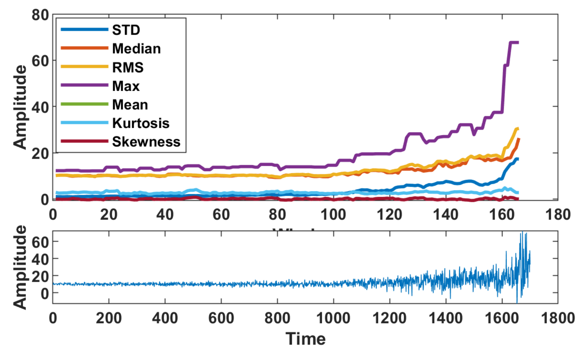
5.2. Extraction of Features for Simulated Signal for Gaussian Noise Case

In Figure 7, seven initially extracted features for Gaussian noise case are plotted.

Based on visual inspection of each statistical feature, three features are selected for further processing, namely STD, RMS, and mean value. They are selected because their shapes are the most similar to the original curve. In Figure 8, a 3D plot of these three features is presented. One may notice that three potential clusters are possible. In the Figure 8 3D plot, one can notice internal dependence/correlation in the data, thus a PCA is applied. Indeed, as one can see in Figure 9, PC1 contains nearly 100 % information. In Figure 10, a comparison of three original features and PC1–PC3 features are presented. One may see a strong correlation between the original features and PC1.

As mentioned above, as original features are highly correlated and the PC1 contains most of the information, the clustering can be done simply. In Figure 11, one can see the trajectory of PC1 (left) and its probability density function. One can easily notice three modes related to three regimes: the first one with amplitude less than 0 is related to regime (good condition), second one with amplitude more than 0 and less than 10 (warning condition) and samples with amplitude above 10 could be considered as regime 3. In Figure 12, the result of clustering in PC1–PC2 space is presented. The degradation development goes from the left side (green cluster) through points cloud in yellow color to several point constituting “Alarm” cluster. As one can see EM, BIRCH and K-means detected three classes with different results. For example, the EM algorithm detected the first and second regimes earlier than other approaches, while K-means and BIRCH discovered the last regime the same. However, the result for the second regime is different. Moreover, BIRCH and K-means recognized more (than EM) points as “Good Condition”, i.e., they may have some trouble recognizing the border between class 1 and class 2 (good and warning) properly.

Finally, in Figure 13, the results of segmentation based on selected clustering algorithm are presented. In Figure 13, one may find a confirmation that K-means and BIRCH recognized too many points as a “good condition” cluster. The change point between the good and warning segment is much later than for the EM algorithm. Hence, one may conclude that the EM algorithm is the best solution here. The exact values of changing point (CP) are presented in

Table 2. Final changing points in case of Gaussian noise.

Algorithm	1st Point	2nd Point
EM	998	1500
K-Means	1240	1570
BIRCH	1390	1580

.

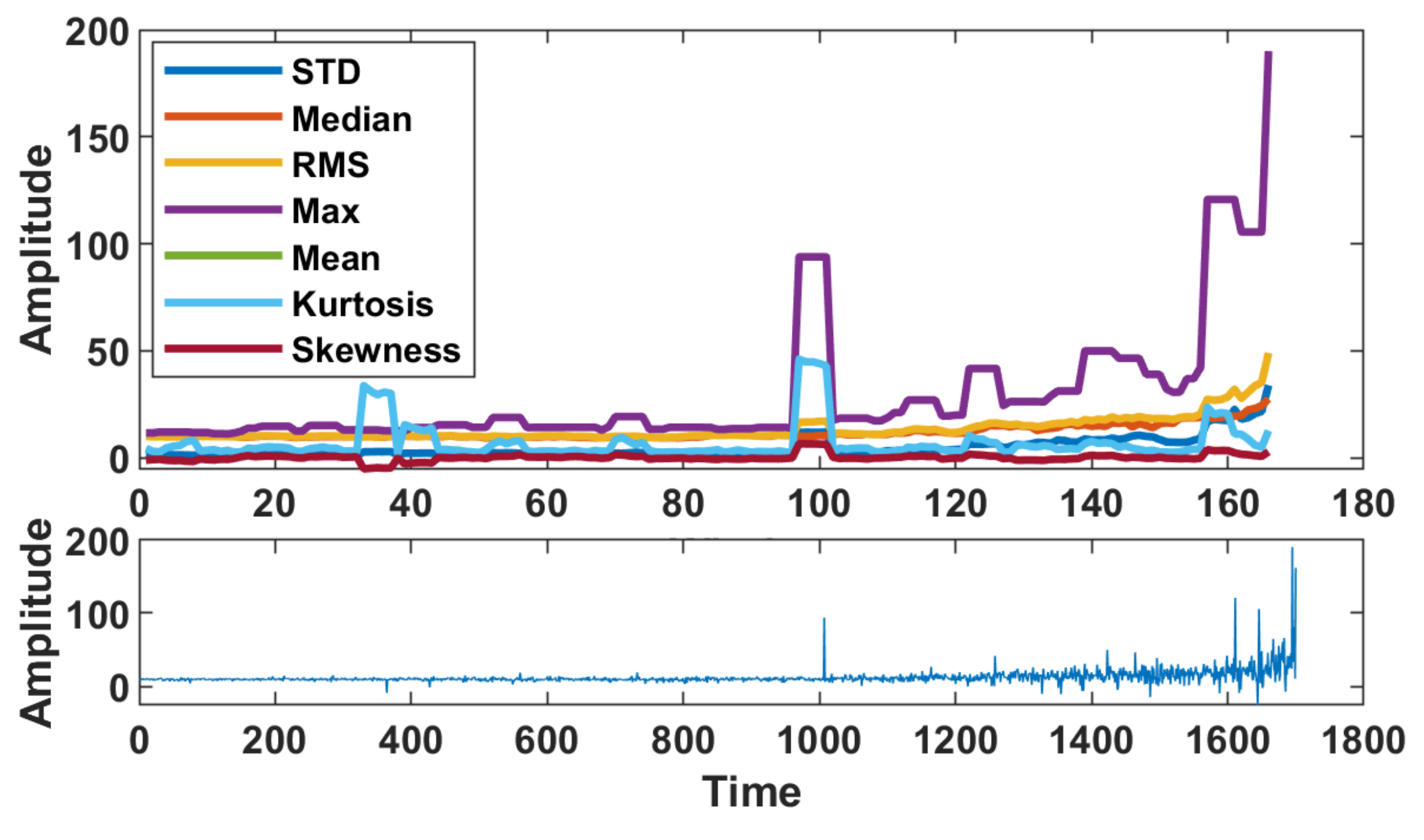
5.3. Extraction of Features from Simulated Signal for Non-Gaussian Noise Case

By analogy, as for the Gaussian case, now the procedure is applied for simulated data with non-Gaussian noise. In Figure 14, all features are presented. It is clear that some of them are not suitable, so they are not considered for later stages. In Figure 15 (left top panel), three selected features are presented. One may conclude that the concept of moving windows and selected statistics as features works properly for Gaussian noise. However, for non-Gaussian noise, when a single outlier occurs, the effect generated by moving window and overlapping produces more artifacts than the original data contain. Hence, while statistics, such as sample mean, are sensitive to a single outlier, also the classical parameters responsible for variance (as sample variance) are not recommended for data with impulsive noise.

In Figure 16, features are plotted in 3D space. Similar to the Gaussian case, regime 3 is clearly noticeable; however, regimes 1 and 2 can be distinguished as well. The impact of distortion of the features does not appear to be significant. In the next step, the data are processed by PCA. Again, the first component (PC1) contains the majority of information; see Figure 17. In Figure 15, one can see that the shape of PC1 is similar to the original data, and PC2 may be useful to recognize a third regime.

In Figure 18, the PC1 time series and its kernel density is presented. One may notice a strong artifact around T = 100. However, based on the empirical probability density function, it is possible to establish threshold values to identify regimes in PC1 (thresholds at c.a PC1 = 0 and PC1 = 10).

In Figure 19, the final results of clustering in the PC domain are demonstrated. The degradation process starts from the healthy stage (green points) to the warning and alarm stages (yellow and red points). As it can be seen in Figure 19, K-means and BIRCH detected regimes as the same while EM algorithm discover the second regime around (−3, −2).

Furthermore, K-means and BIRCH can separate regimes representing the warning and alarm stages, i.e., the yellow and red points. The results of EM for separating yellow and red points are acceptable. Finally, in Figure 20, the last results for simulated data with non-Gaussian noise are presented. It is clearly seen that the results include some mixture of classes that could not be seen in simulations with Gaussian data. Additionally, Figure 20 confirms that the results of clustering with K-means and BIRCH algorithms are correct. However, both of them detected the second stage with significant delay. The delay for EM clustering is less than K-means and BIRCH. The exact values of changing point (CP) are presented in

Table 3. Final changing points in case of non-Gaussian noise.

Algorithm	1st Point	2nd Point
EM	1050	1610
K-Means	1240	1590
BIRCH	1252	1592

.

6. Real Data Analysis

In this section, we present results of application of the proposed procedure to real data sets. Again, two data sets are considered. One of them is related to FEMTO data—one of the most popular data sets widely used as benchmark. It could be interpreted as rather Gaussian case. The second real example is related to wind turbine bearings data. It contains strong non-Gaussian components.

6.1. Real Data with Almost Gaussian Noise

The FEMTO data set [74] was acquired by Franche-Comté Electronics Mechanics Thermal Science and Optics–Sciences and Technologies institute from a PRONOSTIA platform. The test rig is presented in Figure 21. The data set was shared during the prognosis challenge at the conference IEEE PHM 2012. The data set contains 17 historical long-term feature sets describing the degradation of bearing. Two accelerometers and a temperature sensor were used to acquire acceleration and temperature. The speed of the shaft was kept stable during the test. It is assumed that the failure of the bearing occurs when the amplitude of the vibration signal has arrived above 20 g. This data set was used in many publication for segmentation [75,76,77,78,79], construction of the health index [80,81,82,83,84,85,86,87] and predicting RUL [88,89,90,91,92,93].

As one can see, this data set perfectly follows the idea of three regimes: for time 0 to c.a. 12,000, it is nearly flat, then up to t = 27,000 it shows linear increase and then rapid growth Figure 22. Some noise, especially in the middle regime, is also seen; additionally, some small outliers can be noticed. Thus, we consider it as a trend with nearly Gaussian noise. In Figure 23 features extracted using the proposed methodology are plotted. As one can see, RMS and mean value are very similar, and STD reacts significantly only for the third regime. Unfortunately, kurtosis and skewness seem to be not related to degradation. Three features are used for further analysis: STD, RMS and mean value.

In Figure 24, the selected features are plotted together as a 3D plot. As one can expect, data corresponding to the third regime are pretty different compared to regimes 1 and 2, so it can be a bit challenging to recognize regimes 1 and 2.

Next, the PCA is applied. As presented in Figure 25, PC1 contains over 95% of information.

In Figure 26, the results of the PCA analysis are presented. Three original features are plotted together with three principal components. It is clear that the PC1 is following the original features, while PC2 and especially PC3 do not contain too much information. As PC1 is the most informative, one can use the probability density function (PDF) to set up thresholds for regime change point detection. As mentioned above, as original features are highly correlated and the PC1 contains most of the information, the clustering can be done. In Figure 27, one can see the trajectory of PC1 (left) and its PDF. One can easily notice three modes related to three stages: the first one with amplitude less than 0 is related to the healthy (good condition) stage, the second one with amplitude more than 0 and less 0.2 (degradation stage, i.e., warning), and samples with amplitude higher than 0.2 could be considered as critical stages (Alarm).

In Figure 28, the results of the selected clustering techniques are presented. The data with high dispersion correspond to regime no. 3 (red color). Cluster in green color corresponds to the healthy stage. The last one is medium degradation regime (yellow). In general, the EM algorithm provides the most effective result; however, it is not perfect. BIRCH and K-means provide similar results.

In Figure 29, the final result of segmentation is presented. Original data divided into three regimes are plotted with different colors associated to a given regime. As shown in Figure 29, the BIRCH and K-means discovered the second change point much later than what really exists. Additionally, the first change point, which should start around T = 12,000, is detected significantly later by the K-means and BIRCH algorithms. The EM algorithm can detect the third regime (critical stage) correctly, but the first and second regimes are mixed together. It should be highlighted that the difference between the end of regime 1 and the beginning of regime 2 is very small, so there is no surprise that precision is limited here.

However, it is a bit surprising that BIRCH and K-means have some problems with the proper recognition of regime 3. To summarize, the best result is obtained by EM. Exact values of changing point (CP) are presented in

Table 4. Final changing points for the FEMTO data set.

Algorithm	1st Point	2nd Point
EM	13,170	27,120
K-Means	19,780	27,400
BIRCH	20,200	27,800

.

6.2. Real Data with Strong Non-Gaussian Noise

In this section, we provide an example of real data with strongly non-Gaussian noise. This data set contains diagnostic features based on collected vibrations from wind turbine [94] bearings; see Figure 30.

It should be mentioned that this data set has been used for prognosis in several works [94,96,97,98]. In this case, for the construction of the HI, the method proposed in ref. [94] is used. The health index extraction procedure is illustrated on Figure 31. For details of the method, we refer the readers to [94]. The values of inner race energy for a group of measurements for one particular speed (high speed) are demonstrated in Figure 32. In Figure 33, all calculated features are presented. Again, some of them seem not to be useful (does not follow the shape of original data), so they will be ignored for the next step of analysis. In Figure 34, selected features are presented in a 3D plot. Definitely, they are strongly correlated, so the utilization of the PCA is suggested. In Figure 35, the importance of principal components is presented. More than 90 % of the informativeness is included in PC1. In Figure 36, original features and new features (i.e., Principal Components) are presented. One can see that the shape of the PC1 is similar to the original features, while the behavior of PC2 and PC3 is different. Based on PC1 data, the PDF is estimated. It is presented in Figure 37. Threshold values are established experimentally based on PDF of PC1. The right subplot presents segmentation results using colors.

Based on this fact, the wind turbine data set includes many spikes; it is not easy to select the threshold. However, it can be selected approximately: the first one with an amplitude less than 0 is related to the healthy stage, the second one with an amplitude more than 0 and less than 0.2 (degradation stage), and samples with an amplitude higher than 0.2 could be considered as critical stages. Next, three selected features are subjected to clustering algorithms; see Figure 38. All of the algorithms identified three clusters; however, borders for BIRCH and K-means seem to be more clear than for EM. The final results, i.e., clustering-based segmentation for real non-Gaussian data, are presented in Figure 39. As it was concluded for Figure 38, the EM algorithm detects regime 2 too early. More or less, the second regime is discovered by BIRCH and K-means equally; however, the result for detecting the last regime is different. In Figure 39, the final result for the wind turbine data set is presented. Original data divided into three regimes are plotted with different colors associated to the given regime. As shown in Figure 39, the EM could not detect the third regime (critical stage) properly. The other clustering (BIRCH and K-means) approaches are able to divide data into three regimes in a similar way. For this case, the exact changing points are undefined; see

Table 5. Final changing points for wind turbine data set.

Algorithm	1st Point	2nd Point
EM	Undefine	Undefine
K-Means	Undefine	Undefine
BIRCH	Undefine	Undefine

.

7. Conclusions

In the paper, a simple procedure for long-term diagnostic data segmentation is proposed. The procedure is developed to find the regime change point, i.e., borders between three regimes corresponding to three phases of machine life: good condition, slow linear degradation and fast (exponential) degradation.

To achieve the goal, we propose the statistical parameterization of the data performed locally, i.e., using moving short window and then simple techniques for clustering.

It is found that for Gaussian distribution of noise in the data, the efficiency of the method is good—we are able to detect regime change point. As the difference between good condition and beginning of slow degradation is not really significant, border detection is a bit biased. It is not critical (the machine is still in almost good condition).

Unfortunately, non-Gaussian distribution of the noise influences the procedure in several ways. First, the idea of moving window is not really suitable because one outlier will provide several features with bias. Moreover, simple statistics suitable to describe data with Gaussian noise are not optimal for non-Gaussian data. For example, the mean value will be affected by outliers; if the window is short, this influence may be significant. Standard deviation is even more sensitive to outliers, and some heavy-tailed processes cannot use variance at all as it is not defined for such processes. Finally, PCA should not be used in the classical form for heavy-tailed data because it maximize variance (model will follow outliers) and all these steps will impact regime change point detection. This implies a need to search for new approaches. For future work, it is planned that used statistics may be replaced with a robust version (median instead of mean, robust scale instead of variance, etc.). There are many solutions for dimensionality reduction for non-Gaussian data sets. Additionally, clustering methods for non-Gaussian data are available.

The main purpose of this work is to highlight (by simulated and real data analysis) that the non-Gaussian character of the random component in our long-term data should be investigated and evaluated also during the segmentation step before data modeling for machine health prognosis.

References

1. Sikora, G.; Michalak, A.; Bielak, L.; Miśta, P.; Wyłomańska, A. Stochastic modeling of currency exchange rates with novel validation techniques. Phys. A Stat. Mech. Appl. 2019, 523, 1202–1215. [Google Scholar] [CrossRef]
2. Szarek, D.; Bielak, L.; Wyłomańska, A. Long-term prediction of the metals’ prices using non-Gaussian time-inhomogeneous stochastic process. Phys. A Stat. Mech. Appl. 2020, 555. [Google Scholar] [CrossRef]
3. Tapia, C.; Coulton, J.; Saydam, S. Using entropy to assess dynamic behaviour of long-term copper price. Resour. Policy 2020, 66, 101597. [Google Scholar] [CrossRef]
4. Weron, R. Electricity price forecasting: A review of the state-of-the-art with a look into the future. Int. J. Forecast. 2014, 30, 1030–1081. [Google Scholar] [CrossRef] [Green Version]
5. Amasyali, K.; El-Gohary, N. A review of data-driven building energy consumption prediction studies. Renew. Sustain. Energy Rev. 2018, 81, 1192–1205. [Google Scholar] [CrossRef]
6. Zimroz, R.; Bartelmus, W.; Barszcz, T.; Urbanek, J. Diagnostics of bearings in presence of strong operating conditions non-stationarity—A procedure of load-dependent features processing with application to wind turbine bearings. Mech. Syst. Signal Process. 2014, 46, 16–27. [Google Scholar] [CrossRef]
7. Ignasiak, A.; Gomolla, N.; Kruczek, P.; Wylomanska, A.; Zimroz, R. Long term vibration data analysis from wind turbine—Statistical vs. energy based features. Vibroeng. Procedia 2017, 13, 96–102. [Google Scholar] [CrossRef] [Green Version]
8. Wodecki, J.; Stefaniak, P.; Michalak, A.; Wyłomańska, A.; Zimroz, R. Technical condition change detection using Anderson–Darling statistic approach for LHD machines–engine overheating problem. Int. J. Min. Reclam. Environ. 2018, 32, 392–400. [Google Scholar] [CrossRef]
9. Grzesiek, A.; Zimroz, R.; Śliwiński, P.; Gomolla, N.; Wyłomańska, A. Long term belt conveyor gearbox temperature data analysis—Statistical tests for anomaly detection. Meas. J. Int. Meas. Confed. 2020, 165, 108124. [Google Scholar] [CrossRef]
10. Wang, P.; Long, Z.; Wang, G. A hybrid prognostics approach for estimating remaining useful life of wind turbine bearings. Energy Rep. 2020, 6, 173–182. [Google Scholar] [CrossRef]
11. Li, W.; Jiao, Z.; Du, L.; Fan, W.; Zhu, Y. An indirect RUL prognosis for lithium-ion battery under vibration stress using Elman neural network. Int. J. Hydrogen Energy 2019, 44, 12270–12276. [Google Scholar] [CrossRef]
12. Staszewski, W.; Tomlinson, G. Local tooth fault detection in gearboxes using a moving window procedure. Mech. Syst. Signal Process. 1997, 11, 331–350. [Google Scholar] [CrossRef]
13. Marcjasz, G.; Serafin, T.; Weron, R. Selection of calibration windows for day-ahead electricity price forecasting. Energies 2018, 11, 2364. [Google Scholar] [CrossRef] [Green Version]
14. Allen, J. Short Term Spectral Analysis, Synthesis, and Modification by Discrete Fourier Transform. IEEE Trans. Acoust. Speech Signal Process. 1977, 25, 235–238. [Google Scholar] [CrossRef]
15. Yan, H.; Qin, Y.; Xiang, S.; Wang, Y.; Chen, H. Long-term gear life prediction based on ordered neurons LSTM neural networks. Measurement 2020, 165, 108205. [Google Scholar] [CrossRef]
16. Tamilselvan, P.; Wang, Y.; Wang, P. Deep belief network based state classification for structural health diagnosis. In Proceedings of the 2012 IEEE Aerospace Conference, Big Sky, MT, USA, 3–10 March 2012; pp. 1–11. [Google Scholar]
17. Liu, J.; Lei, F.; Pan, C.; Hu, D.; Zuo, H. Prediction of remaining useful life of multi-stage aero-engine based on clustering and LSTM fusion. Reliab. Eng. Syst. Saf. 2021, 214, 107807. [Google Scholar] [CrossRef]
18. Singh, J.; Darpe, A.; Singh, S.P. Bearing remaining useful life estimation using an adaptive data-driven model based on health state change point identification and K-means clustering. Meas. Sci. Technol. 2020, 31, 085601. [Google Scholar] [CrossRef]
19. Mao, W.; He, J.; Sun, B.; Wang, L. Prediction of Bearings Remaining Useful Life Across Working Conditions Based on Transfer Learning and Time Series Clustering. IEEE Access 2021, 9, 135285–135303. [Google Scholar] [CrossRef]
20. Sharanya, S.; Venkataraman, R.; Murali, G. Estimation of Remaining Useful Life of Bearings Using Reduced Affinity Propagated Clustering. J. Eng. Sci. Technol. 2021, 16, 3737–3756. [Google Scholar]
21. Javed, K.; Gouriveau, R.; Zerhouni, N. A new multivariate approach for prognostics based on extreme learning machine and fuzzy clustering. IEEE Trans. Cybern. 2015, 45, 2626–2639. [Google Scholar] [CrossRef] [Green Version]
22. Chen, Z.; Wu, M.; Zhao, R.; Guretno, F.; Yan, R.; Li, X. Machine remaining useful life prediction via an attention-based deep learning approach. IEEE Trans. Ind. Electron. 2020, 68, 2521–2531. [Google Scholar] [CrossRef]
23. Mousavi, S.M.; Abdullah, S.; Niaki, S.T.A.; Banihashemi, S. An intelligent hybrid classification algorithm integrating fuzzy rule-based extraction and harmony search optimization: Medical diagnosis applications. Knowl.-Based Syst. 2021, 220, 106943. [Google Scholar] [CrossRef]
24. Yu, W.; Kim, I.Y.; Mechefske, C. Analysis of different RNN autoencoder variants for time series classification and machine prognostics. Mech. Syst. Signal Process. 2021, 149, 107322. [Google Scholar] [CrossRef]
25. Baptista, M.L.; Henriques, E.M.; Prendinger, H. Classification prognostics approaches in aviation. Measurement 2021, 182, 109756. [Google Scholar] [CrossRef]
26. Stock, S.; Pohlmann, S.; Günter, F.J.; Hille, L.; Hagemeister, J.; Reinhart, G. Early quality classification and prediction of battery cycle life in production using machine learning. J. Energy Storage 2022, 50, 104144. [Google Scholar] [CrossRef]
27. Buchaiah, S.; Shakya, P. Bearing fault diagnosis and prognosis using data fusion based feature extraction and feature selection. Measurement 2022, 188, 110506. [Google Scholar] [CrossRef]
28. Aminikhanghahi, S.; Cook, D.J. A survey of methods for time series change point detection. Knowl. Inf. Syst. 2017, 51, 339–367. [Google Scholar] [CrossRef] [PubMed] [Green Version]
29. Prakash, A.; James, N.; Menzies, M.; Francis, G. Structural clustering of volatility regimes for dynamic trading strategies. Appl. Math. Financ. 2022, 28, 236–274. [Google Scholar] [CrossRef]
30. Das, S. Blind Change Point Detection and Regime Segmentation Using Gaussian Process Regression. Ph.D. Thesis, University of South Carolina, Columbia, SC, USA, 2017. [Google Scholar]
31. Abonyi, J.; Feil, B.; Nemeth, S.; Arva, P. Fuzzy clustering based segmentation of time-series. In Proceedings of the International Symposium on Intelligent Data Analysis, Berlin, Germany, 28–30 August 2003; Springer: Berlin/Heidelberg, Germany, 2003; pp. 275–285. [Google Scholar]
32. Tseng, V.S.; Chen, C.H.; Huang, P.C.; Hong, T.P. Cluster-based genetic segmentation of time series with DWT. Pattern Recognit. Lett. 2009, 30, 1190–1197. [Google Scholar] [CrossRef]
33. Samé, A.; Chamroukhi, F.; Govaert, G.; Aknin, P. Model-based clustering and segmentation of time series with changes in regime. Adv. Data Anal. Classif. 2011, 5, 301–321. [Google Scholar] [CrossRef] [Green Version]
34. Keogh, E.J.; Pazzani, M.J. An Enhanced Representation of Time Series Which Allows Fast and Accurate Classification, Clustering and Relevance Feedback. Proc. KDD 1998, 98, 239–243. [Google Scholar]
35. Tseng, V.S.; Chen, C.H.; Chen, C.H.; Hong, T.P. Segmentation of time series by the clustering and genetic algorithms. In Proceedings of the Sixth IEEE International Conference on Data Mining-Workshops (ICDMW’06), Hong Kong, China, 18–22 December 2006; pp. 443–447. [Google Scholar]
36. Wood, K.; Roberts, S.; Zohren, S. Slow momentum with fast reversion: A trading strategy using deep learning and changepoint detection. J. Financ. Data Sci. 2022, 4, 111–129. [Google Scholar] [CrossRef]
37. Liu, X.; Zhang, T. Estimating change-point latent factor models for high-dimensional time series. J. Stat. Plan. Inference 2022, 217, 69–91. [Google Scholar] [CrossRef]
38. Ge, X.; Lin, A. Kernel change point detection based on convergent cross mapping. Commun. Nonlinear Sci. Numer. Simul. 2022, 109, 106318. [Google Scholar] [CrossRef]
39. Kucharczyk, D.; Wyłomańska, A.; Obuchowski, J.; Zimroz, R.; Madziarz, M. Stochastic Modelling as a Tool for Seismic Signals Segmentation. Shock Vib. 2016, 2016, 8453426. [Google Scholar] [CrossRef] [Green Version]
40. Gąsior, K.; Urbańska, H.; Grzesiek, A.; Zimroz, R.; Wyłomańska, A. Identification, decomposition and segmentation of impulsive vibration signals with deterministic components—A sieving screen case study. Sensors 2020, 20, 5648. [Google Scholar] [CrossRef]
41. Grzesiek, A.; Gasior, K.; Wyłomańska, A.; Zimroz, R. Divergence-based segmentation algorithm for heavy-tailed acoustic signals with time-varying characteristics. Sensors 2021, 21, 8487. [Google Scholar] [CrossRef]
42. Wen, Y.; Wu, J.; Das, D.; Tseng, T.L. Degradation modeling and RUL prediction using Wiener process subject to multiple change points and unit heterogeneity. Reliab. Eng. Syst. Saf. 2018, 176, 113–124. [Google Scholar] [CrossRef]
43. Lei, Y.; Li, N.; Guo, L.; Li, N.; Yan, T.; Lin, J. Machinery health prognostics: A systematic review from data acquisition to RUL prediction. Mech. Syst. Signal Process. 2018, 104, 799–834. [Google Scholar] [CrossRef]
44. Heng, A.; Zhang, S.; Tan, A.; Mathew, J. Rotating machinery prognostics: State of the art, challenges and opportunities. Mech. Syst. Signal Process. 2009, 23, 724–739. [Google Scholar] [CrossRef]
45. Sikorska, J.; Hodkiewicz, M.; Ma, L. Prognostic modelling options for remaining useful life estimation by industry. Mech. Syst. Signal Process. 2011, 25, 1803–1836. [Google Scholar] [CrossRef]
46. Lee, J.; Wu, F.; Zhao, W.; Ghaffari, M.; Liao, L.; Siegel, D. Prognostics and health management design for rotary machinery systems—Reviews, methodology and applications. Mech. Syst. Signal Process. 2014, 42, 314–334. [Google Scholar] [CrossRef]
47. Si, X.S.; Wang, W.; Hu, C.H.; Zhou, D.H. Remaining useful life estimation—A review on the statistical data driven approaches. Eur. J. Oper. Res. 2011, 213, 1–14. [Google Scholar] [CrossRef]
48. Kan, M.; Tan, A.; Mathew, J. A review on prognostic techniques for non-stationary and non-linear rotating systems. Mech. Syst. Signal Process. 2015, 62, 1–20. [Google Scholar] [CrossRef]
49. Reuben, L.; Mba, D. Diagnostics and prognostics using switching Kalman filters. Struct. Health Monit. 2014, 13, 296–306. [Google Scholar] [CrossRef]
50. Lim, C.; Mba, D. Switching Kalman filter for failure prognostic. Mech. Syst. Signal Process. 2015, 52-53, 426–435. [Google Scholar] [CrossRef]
51. Wodecki, J.; Stefaniak, P.; Obuchowski, J.; Wylomanska, A.; Zimroz, R. Combination of principal component analysis and time-frequency representations of multichannel vibration data for gearbox fault detection. J. Vibroeng. 2016, 18, 2167–2175. [Google Scholar]
52. Wikipedia. Principal Component Analysis. 2016. Available online: https://en.wikipedia.org/wiki/Principal_component_analysis (accessed on 9 May 2022).
53. Peter, D.H. Kernel estimation of a distribution function. Commun. Stat.-Theory Methods 1985, 14, 605–620. [Google Scholar] [CrossRef]
54. Silverman, B.W. Density estimation for statistics and data analysis. In Monographs on Statistics and Applied Probability; CRC Press: Boca Raton, FL, USA, 1986; Volume 26. [Google Scholar]
55. Jin, R.; Goswami, A.; Agrawal, G. Fast and exact out-of-core and distributed k-means clustering. Knowl. Inf. Syst. 2006, 10, 17–40. [Google Scholar] [CrossRef] [Green Version]
56. Likas, A.; Vlassis, N.; Verbeek, J.J. The global k-means clustering algorithm. Pattern Recognit. 2003, 36, 451–461. [Google Scholar] [CrossRef] [Green Version]
57. Hartigan, J.A.; Wong, M.A. Algorithm AS 136: A k-means clustering algorithm. J. R. Stat. Soc. Ser. C Appl. Stat. 1979, 28, 100–108. [Google Scholar] [CrossRef]
58. Kodinariya, T.M.; Makwana, P.R. Review on determining number of Cluster in K-Means Clustering. Int. J. 2013, 1, 90–95. [Google Scholar]
59. Zhang, T.; Ramakrishnan, R.; Livny, M. BIRCH: A new data clustering algorithm and its applications. Data Min. Knowl. Discov. 1997, 1, 141–182. [Google Scholar] [CrossRef]
60. Zhang, T.; Ramakrishnan, R.; Livny, M. BIRCH: An efficient data clustering method for very large databases. ACM Sigmod Rec. 1996, 25, 103–114. [Google Scholar] [CrossRef]
61. Madan, S.; Dana, K.J. Modified balanced iterative reducing and clustering using hierarchies (m-BIRCH) for visual clustering. Pattern Anal. Appl. 2016, 19, 1023–1040. [Google Scholar] [CrossRef]
62. Liu, S.; Cao, D.; An, P.; Yang, X.; Zhang, M. Automatic fault detection based on the unsupervised seismic attributes clustering. In Proceedings of the SEG 2018 Workshop: SEG Maximizing Asset Value Through Artificial Intelligence and Machine Learning, Beijing, China, 17–19 September 2018; Society of Exploration Geophysicists: Houston, TX, USA; Chinese Geophysical Society: Beijing, China, 2018; pp. 56–59. [Google Scholar]
63. Dempster, A.P.; Laird, N.M.; Rubin, D.B. Maximum likelihood from incomplete data via the EM algorithm. J. R. Stat. Soc. Ser. B Methodol. 1977, 39, 1–38. [Google Scholar]
64. Sundberg, R. Maximum likelihood theory for incomplete data from an exponential family. Scand. J. Stat. 1974, 1, 49–58. [Google Scholar]
65. Maugis, C.; Celeux, G.; Martin-Magniette, M.L. Variable selection for clustering with Gaussian mixture models. Biometrics 2009, 65, 701–709. [Google Scholar] [CrossRef] [Green Version]
66. McLachlan, G.J.; Basford, K.E. Mixture Models: Inference and Applications to Clustering; M. Dekker: New York, NY, USA, 1988; Volume 38. [Google Scholar]
67. Biernacki, C.; Celeux, G.; Govaert, G. Assessing a mixture model for clustering with the integrated completed likelihood. IEEE Trans. Pattern Anal. Mach. Intell. 2000, 22, 719–725. [Google Scholar] [CrossRef]
68. Kruczek, P.; Wodecki, J.; Wyłomanska, A.; Zimroz, R.; Gryllias, K.; Grobli, N. Multi-fault diagnosis based on bi-frequency cyclostation-ary maps clustering. In Proceedings of the ISMA2018-USD2018, Leuven, Belgium, 17–19 September 2018; pp. 981–990. [Google Scholar]
69. Hebda-Sobkowicz, J.; Zimroz, R.; Wyłomańska, A.; Antoni, J. Infogram performance analysis and its enhancement for bearings diagnostics in presence of non-Gaussian noise. Mech. Syst. Signal Process. 2022, 170, 108764. [Google Scholar] [CrossRef]
70. Wodecki, J.; Michalak, A.; Wyłomańska, A.; Zimroz, R. Influence of non-Gaussian noise on the effectiveness of cyclostationary analysis—Simulations and real data analysis. Measurement 2021, 171, 108814. [Google Scholar] [CrossRef]
71. Kruczek, P.; Zimroz, R.; Antoni, J.; Wyłomańska, A. Generalized spectral coherence for cyclostationary signals with α-stable distribution. Mech. Syst. Signal Process. 2021, 159, 107737. [Google Scholar] [CrossRef]
72. Khinchine, A.Y.; Lévy, P. Sur les lois stables. CR Acad. Sci. Paris 1936, 202, 374–376. [Google Scholar]
73. Burnecki, K.; Wyłomańska, A.; Beletskii, A.; Gonchar, V.; Chechkin, A. Recognition of stable distribution with Lévy index α close to 2. Phys. Rev. E 2012, 85, 056711. [Google Scholar] [CrossRef] [Green Version]
74. Nectoux, P.; Gouriveau, R.; Medjaher, K.; Ramasso, E.; Chebel-Morello, B.; Zerhouni, N.; Varnier, C. PRONOSTIA: An experimental platform for bearings accelerated degradation tests. In Proceedings of the IEEE International Conference on Prognostics and Health Management, PHM’12, Denver, CO, USA, 18–21 June 2012; pp. 1–8. [Google Scholar]
75. Liu, Z.; Zuo, M.J.; Qin, Y. Remaining useful life prediction of rolling element bearings based on health state assessment. Proc. Inst. Mech. Eng. Part C J. Mech. Eng. Sci. 2016, 230, 314–330. [Google Scholar] [CrossRef] [Green Version]
76. Kimotho, J.K.; Sondermann-Wölke, C.; Meyer, T.; Sextro, W. Machinery Prognostic Method Based on Multi-Class Support Vector Machines and Hybrid Differential Evolution–Particle Swarm Optimization. Chem. Eng. Trans. 2013, 33, 619–624. [Google Scholar]
77. Zurita, D.; Carino, J.A.; Delgado, M.; Ortega, J.A. Distributed neuro-fuzzy feature forecasting approach for condition monitoring. In Proceedings of the 2014 IEEE Emerging Technology and Factory Automation (ETFA), Barcelona, Spain, 16–19 September 2014; pp. 1–8. [Google Scholar]
78. Guo, L.; Gao, H.; Huang, H.; He, X.; Li, S. Multifeatures fusion and nonlinear dimension reduction for intelligent bearing condition monitoring. Shock Vib. 2016, 2016, 4632562. [Google Scholar] [CrossRef] [Green Version]
79. Jin, X.; Sun, Y.; Que, Z.; Wang, Y.; Chow, T.W. Anomaly detection and fault prognosis for bearings. IEEE Trans. Instrum. Meas. 2016, 65, 2046–2054. [Google Scholar] [CrossRef]
80. Mosallam, A.; Medjaher, K.; Zerhouni, N. Time series trending for condition assessment and prognostics. J. Manuf. Technol. Manag. 2014, 25, 550–567. [Google Scholar] [CrossRef]
81. Loutas, T.H.; Roulias, D.; Georgoulas, G. Remaining useful life estimation in rolling bearings utilizing data-driven probabilistic e-support vectors regression. IEEE Trans. Reliab. 2013, 62, 821–832. [Google Scholar] [CrossRef]
82. Javed, K.; Gouriveau, R.; Zerhouni, N.; Nectoux, P. Enabling health monitoring approach based on vibration data for accurate prognostics. IEEE Trans. Ind. Electron. 2014, 62, 647–656. [Google Scholar] [CrossRef] [Green Version]
83. Singleton, R.K.; Strangas, E.G.; Aviyente, S. Extended Kalman filtering for remaining-useful-life estimation of bearings. IEEE Trans. Ind. Electron. 2014, 62, 1781–1790. [Google Scholar] [CrossRef]
84. Zhang, B.; Zhang, L.; Xu, J. Degradation feature selection for remaining useful life prediction of rolling element bearings. Qual. Reliab. Eng. Int. 2016, 32, 547–554. [Google Scholar] [CrossRef]
85. Hong, S.; Zhou, Z.; Zio, E.; Wang, W. An adaptive method for health trend prediction of rotating bearings. Digit. Signal Process. 2014, 35, 117–123. [Google Scholar] [CrossRef]
86. Lei, Y.; Li, N.; Gontarz, S.; Lin, J.; Radkowski, S.; Dybala, J. A model-based method for remaining useful life prediction of machinery. IEEE Trans. Reliab. 2016, 65, 1314–1326. [Google Scholar] [CrossRef]
87. Nie, Y.; Wan, J. Estimation of remaining useful life of bearings using sparse representation method. In Proceedings of the 2015 Prognostics and System Health Management Conference (PHM), Beijing, China, 21–23 October 2015; pp. 1–6. [Google Scholar]
88. Li, H.; Wang, Y. Rolling bearing reliability estimation based on logistic regression model. In Proceedings of the 2013 International Conference on Quality, Reliability, Risk, Maintenance, and Safety Engineering (QR2MSE), Chengdu, China, 15–18 July 2013; pp. 1730–1733. [Google Scholar]
89. Huang, Z.; Xu, Z.; Ke, X.; Wang, W.; Sun, Y. Remaining useful life prediction for an adaptive skew-Wiener process model. Mech. Syst. Signal Process. 2017, 87, 294–306. [Google Scholar] [CrossRef]
90. Wang, Y.; Peng, Y.; Zi, Y.; Jin, X.; Tsui, K.L. A two-stage data-driven-based prognostic approach for bearing degradation problem. IEEE Trans. Ind. Inform. 2016, 12, 924–932. [Google Scholar] [CrossRef]
91. Pan, Y.; Er, M.J.; Li, X.; Yu, H.; Gouriveau, R. Machine health condition prediction via online dynamic fuzzy neural networks. Eng. Appl. Artif. Intell. 2014, 35, 105–113. [Google Scholar] [CrossRef]
92. Wang, L.; Zhang, L.; Wang, X.z. Reliability estimation and remaining useful lifetime prediction for bearing based on proportional hazard model. J. Cent. South Univ. 2015, 22, 4625–4633. [Google Scholar] [CrossRef]
93. Xiao, L.; Chen, X.; Zhang, X.; Liu, M. A novel approach for bearing remaining useful life estimation under neither failure nor suspension histories condition. J. Intell. Manuf. 2017, 28, 1893–1914. [Google Scholar] [CrossRef]
94. Bechhoefer, E.; Schlanbusch, R. Generalized Prognostic Algorithm Implementing Kalman Smoother. IFAC-PapersOnLine 2015, 48, 97–104. [Google Scholar] [CrossRef]
95. Saidi, L.; Ali, J.B.; Bechhoefer, E.; Benbouzid, M. Particle filter-based prognostic approach for high-speed shaft bearing wind turbine progressive degradations. In Proceedings of the IECON 2017—43rd Annual Conference of the IEEE Industrial Electronics Society, Beijing, China, 29 October–1 November 2017; pp. 8099–8104. [Google Scholar]
96. Saidi, L.; Ali, J.B.; Bechhoefer, E.; Benbouzid, M. Wind turbine high-speed shaft bearings health prognosis through a spectral Kurtosis-derived indices and SVR. Appl. Acoust. 2017, 120, 1–8. [Google Scholar] [CrossRef]
97. Saidi, L.; Bechhoefer, E.; Ali, J.B.; Benbouzid, M. Wind turbine high-speed shaft bearing degradation analysis for run-to-failure testing using spectral kurtosis. In Proceedings of the 2015 16th International Conference on Sciences and Techniques of Automatic Control and Computer Engineering (STA), Monastir, Tunisia, 21–23 December 2015; pp. 267–272. [Google Scholar]
98. Ali, J.B.; Saidi, L.; Harrath, S.; Bechhoefer, E.; Benbouzid, M. Online automatic diagnosis of wind turbine bearings progressive degradations under real experimental conditions based on unsupervised machine learning. Appl. Acoust. 2018, 132, 167–181. [Google Scholar]
Figure 1. Long-term data variation model used in this paper.
Applsci 12 06766 g001
Figure 2. A block diagram of the procedure.
Applsci 12 06766 g002
Figure 3. The idea of segmentation and parametrisation long-term data.
Applsci 12 06766 g003
Figure 4. The geometric interpretation of PCA [52].
Applsci 12 06766 g004
Figure 5. Input simulated data for Gaussian noise. (a) deterministic component, (b) random component, (c) simulation of the signal.
Applsci 12 06766 g005
Figure 6. Input simulated data for non-Gaussian α -stable noise with α = 1.8 . (a) deterministic component, (b) random component, (c) simulation of the signal.
Applsci 12 06766 g006
Figure 7. Statistical features for simulation signal in presence of Gaussian noise.
Applsci 12 06766 g007
Figure 8. Features space for simulation signal in presence of Gaussian noise.
Applsci 12 06766 g008
Figure 9. PCA score for simulation signal in presence of Gaussian noise.
Applsci 12 06766 g009
Figure 10. PCA of raw features for simulation signal in presence of Gaussian noise.
Applsci 12 06766 g010
Figure 11. PC1 time series, its kernel density of PC 1 and final segmentation results for simulation signal in presence of Gaussian noise.
Applsci 12 06766 g011
Figure 12. The output of clustering algorithms for simulation signal in presence of Gaussian noise: (a) EM result, (b) K-Means Result, (c) BIRCH result.
Applsci 12 06766 g012
Figure 13. The expansion of the clustering result to whole of data for simulated signal in presence of Gaussian noise: (a) results for EM algorithm, (b) results for K-Means algorithm, (c) results for BIRCH algorithm.
Applsci 12 06766 g013
Figure 14. Statistical features obtained for non-Gaussian α -stable simulation case.
Applsci 12 06766 g014
Figure 15. PCA of stochastic features for simulation signal in presence of non-Gaussian noise.
Applsci 12 06766 g015
Figure 16. Features space for simulation signal in presence of non-Gaussian noise.
Applsci 12 06766 g016
Figure 17. PCA score in case of simulation noise is non-Gaussian.
Applsci 12 06766 g017
Figure 18. PC1 time series, its Kernel density of features and final results of segmentation expressed by colors for simulation signal in presence of non-Gaussian noise.
Applsci 12 06766 g018
Figure 19. The output of clustering algorithm for simulation signal in presence of non-Gaussian noise: (a) results for EM algorithm, (b) results for K-Means algorithm, (c) results for BIRCH algorithm.
Applsci 12 06766 g019
Figure 20. The expansion of clustering algorithm on whole of data for simulation signal in presence of non-Gaussian noise: (a) results for EM algorithm, (b) results for K-Means algorithm, (c) results for BIRCH algorithm.
Applsci 12 06766 g020
Figure 21. Overview of PRONOSTIA FEMTO data set [74].
Applsci 12 06766 g021
Figure 22. Health index (RMS) from FEMTO data set: (a) representation of Health index with points cloud, (b) representation of Health index with line.
Applsci 12 06766 g022
Figure 23. Features extracted according to proposed methodology for FEMTO data set.
Applsci 12 06766 g023
Figure 24. Features space FEMTO data set.
Applsci 12 06766 g024
Figure 25. PCA scores for FEMTO data set.
Applsci 12 06766 g025
Figure 26. Results of PCA applied to FEMTO data set.
Applsci 12 06766 g026
Figure 27. PC1 of raw FEMTO data, its kernel density and segmentation results marked by colors.
Applsci 12 06766 g027
Figure 28. The output of clustering algorithm for FEMTO data set: (a) results for EM algorithm, (b) results for K-Means algorithm, (c) results for BIRCH algorithm.
Applsci 12 06766 g028
Figure 29. The segmentation results based on clustering algorithm over whole of FEMTO data set: (a) results for EM algorithm, (b) results for K-Means algorithm, (c) results for Birch algorithm.
Applsci 12 06766 g029
Figure 30. An experimental setup and picture of damage of bearing inner race [95].
Applsci 12 06766 g030
Figure 31. Health index extraction for wind turbine data set [94].
Applsci 12 06766 g031
Figure 32. Heath index of wind turbine data set.
Applsci 12 06766 g032
Figure 33. Wind turbine stochastic features.
Applsci 12 06766 g033
Figure 34. Wind turbine stochastic features space.
Applsci 12 06766 g034
Figure 35. Wind turbine PCA score.
Applsci 12 06766 g035
Figure 36. Wind turbine PCA.
Applsci 12 06766 g036
Figure 37. Wind turbine kernel density based PC1.
Applsci 12 06766 g037
Figure 38. Wind turbine clustering: (a) results for EM algorithm, (b) results for K-Means algorithm, (c) results for Birch algorithm.
Applsci 12 06766 g038
Figure 39. The segmentation results based on clustering algorithm over whole of wind turbine data: (a) results for EM algorithm, (b) results for K-Means algorithm, (c) results for Birch algorithm.
Applsci 12 06766 g039