Article

A Hybrid Neural Network Model for Predicting Bottomhole Pressure in Managed Pressure Drilling

1
School of Petroleum Engineering, China University of Petroleum (Beijing), Beijing 102249, China
2
State Key Laboratory of Petroleum Resources and Prospecting, China University of Petroleum, Beijing 102249, China
*
Author to whom correspondence should be addressed.
Appl. Sci. 2022, 12(13), 6728; https://doi.org/10.3390/app12136728
Submission received: 17 May 2022 / Revised: 20 June 2022 / Accepted: 22 June 2022 / Published: 2 July 2022

Abstract

:

Featured Application

This article highlights the feasibility and advantages of using hybrid optimization network models to predict bottomhole pressure under managed pressure drilling.

Abstract

Managed pressure drilling (MPD) is an essential technology for safe and efficient drilling in deep high-temperature and high-pressure formations with narrow safety pressure windows. However, the complex conditions in deep wells make the mechanism of multiphase flow in drilling annulus complicated and increase the difficulty for accurate prediction of bottomhole pressure (BHP). Recently, an increasing volume of research shows that intelligent technology is an efficient means of accurately predicting BHP. However, few studies have focused on the temporal properties and variation mechanism of BHP. In this paper, hybrid neural network prediction models based on the multi-branch parallel are established by combining the different advantages of back propagation (BP), long short-term memory (LSTM), and a one-dimensional convolutional neural network (1DCNN) model. The results show that the relative error of the best model is about 70% lower than the optimal single intelligent model. Preliminary experimental results reveal that the hybrid models combine the advantages of different single models, which is more accurate and robust for extracting the temporal features of MWD. Finally, based on the trend analysis, the validity of the hybrid model is further verified. This study provides a reference for solving the problem of optimizing temporal characteristics and guidance for fine pressure control in complex formations.

1. Introduction

Real-time monitoring of BHP is an important reference for the drilling program design, optimization of drilling parameters, and the dynamic regulation of production programs, which can provide a basic guarantee for safe, efficient drilling and the development of oil and gas [1]. For deep high-temperature and high-pressure drilling, accurate and efficient calculation of BHP is more critical to ensure drilling safety. The traditional methods of estimating BHP mainly include mechanistic model-based calculation and using gauge or well testing, but there are major economic and technical limitations in this method; although the mechanistic model calculation method [2,3,4,5,6,7,8] is less costly, it is difficult to consider all complex environmental conditions simultaneously. Therefore, most of the methods can hardly process a large variety of datasets and only perform well under certain conditions.
Recently, the introduction of intelligence technology has realized accurate and efficient prediction of BHP based on surface monitoring data and provides scientific basis and technical support for safe drilling and efficient production. Many researchers have conducted exploratory research on intelligent prediction methods of BHP. One of the most representative is the use of Artificial Neural Network (ANN) techniques. As early as 1995, Ternyik et al. [9] established a prediction model of BHP based on ANN according to the three-phase flow law of oil, gas and water, and compared the field data to verify the feasibility of the neural network model of BHP. Subsequently, several scholars have used machine learning methods and built different types of ANN models to predict BHP, such as Mohammadpoor et al. [10], Jahanandish et al. [11], Chen et al. [12], Spesivtsev et al. [13], Mask et al. [14], Sami and Ibrahim [1], and Okoro et al. [15]. The prediction results from these studies all indicate the following similarities:
  • The ANN models have significantly improved the accuracy and efficiency of BHP compared with traditional calculation modeling, overcome the limitations of empirical and mechanistic models, and even replaced the function of downhole sensors.
  • These models scarcely considered the temporal properties of datasets and variation mechanism of BHP.
Furthermore, some researchers highlighted that the optimization algorithms also played a significant role in improving the performance of the intelligent prediction model of drilling BHP. Several studies on BHP prediction using optimization algorithms, for instance, particle swarm optimization algorithm [16], gray wolves optimization algorithm [17], ant swarm algorithm [18], and genetic algorithm [19,20,21], have revealed that optimization algorithms combined with the traditional neural network models have higher precision and stronger robustness. Compared with a single solvable model, this model combined with the optimization algorithm can solve issues globally and is independent of the initial conditions.
In fact, with the development of artificial intelligence, more and more researchers have begun to explore the integration of intelligence and mechanisms to further improve the performance of intelligent models such as data fusion, a combination of data and mechanism, etc. In terms of BHP prediction, the following research has been conducted. Fruhwirth et al. [22] integrated multiple flow parameters into comprehensive parameters such as wellbore Reynolds number or dimensionless diameter, which also improved the generalization ability of the model. Elzenary et al. [23] presented a principal component analysis to reduce the number of input parameters, simplify the model structure, and weaken the overfitting of the model. Al Shehri et al. [24] considered the mechanism relations among input parameters, constructed neural network sub-modules, and integrated all sub-modules into a functional neural network system, which improved the model’s mechanism description. Adaptive fuzzy logic is another effective way to improve the performance of neural networks [21]. The fusion of mechanism and data can improve the stability, generalization, and accuracy of the model. Based on flow pattern recognition, Li et al. [25] developed the neural network models of circulating pressure drop under different flow patterns and supplemented the multiphase flow formula to realize the separate calculation of BHP drop in different well sections, extending the applicable conditions of the intelligent method. Gola et al. [26] proposed the grey box theory and innovated the combination method of mechanisms and the intelligent model.
MPD data have both strong and weak time-series feature parameters, such as drilling fluid rheological parameters, which play a key role [27], and the single intelligent prediction models, such as BP, LSTM, and CNN, lack the ability to capture potential information, while the parallel dual-branch networks can simultaneously capture the strong and weak features of time-series data in order to mine more related information of time-series data, thereby reducing information loss.
Based on the advantages of the single intelligent models to capture different characteristics, hybrid optimization parallel models are established in this paper. This method can fully identify the time-series characteristics of the data and effectively capture the subtle changes behind the data. This research can be applied to optimally solve temporal problems and provides a reference for precise pressure control in drilling.

2. Theory Background

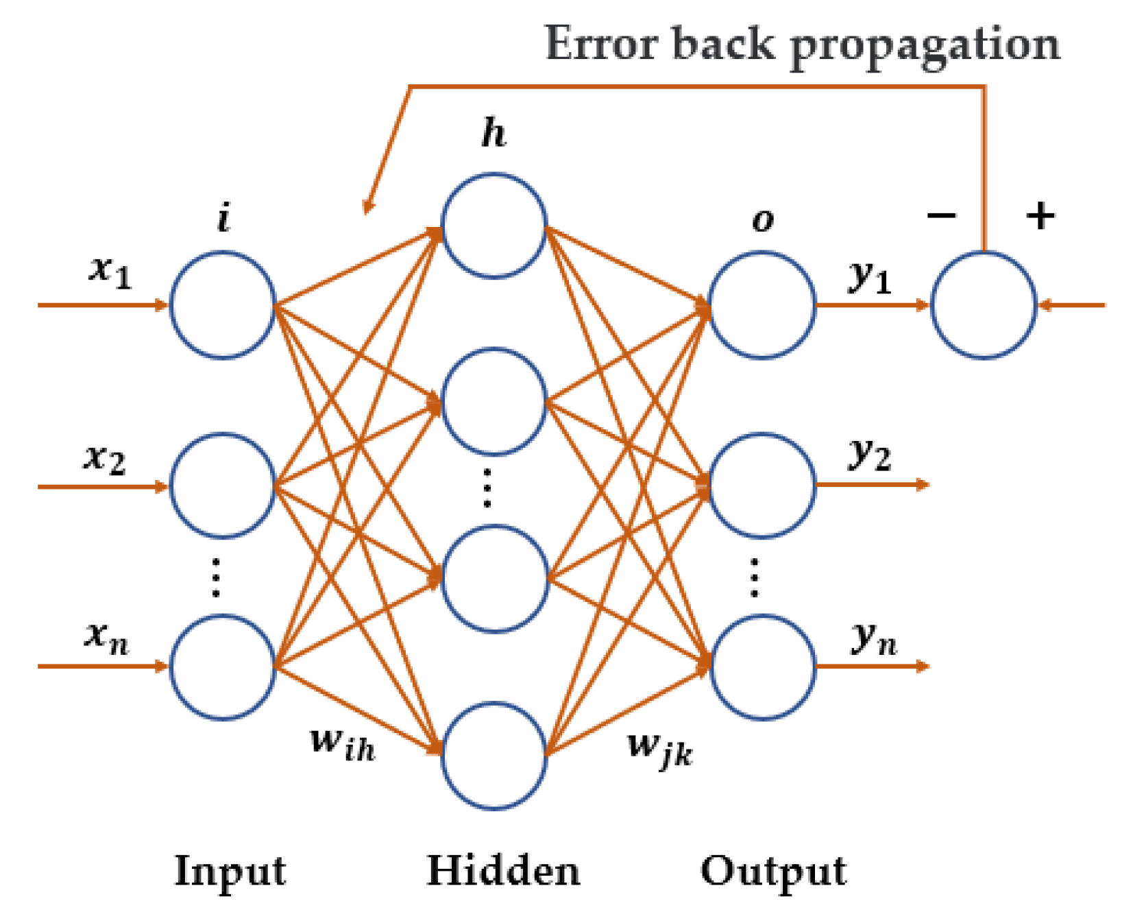
2.1. BP Neural Network

The BP neural network in Figure 1 is a multilayer feedforward neural network trained according to error backward propagation algorithm [28]. It is good at capturing the potential relationship between input and output. With its arbitrarily complex network structure and powerful nonlinear mapping ability, it is one of the most widely used neural networks. However, the BP neural network can only accept the input of a fixed dimension, thus generating the output of a fixed dimension, and the completion process is point-to-point mapping, unable to consider the temporal properties of BHP and unable to analyze the relationship in the contextual information of the time series data.

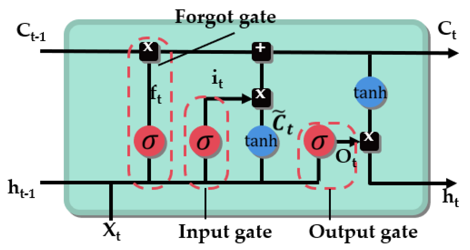
2.2. LSTM Neural Network

Different from feedforward neural networks, recurrent neural network is a basic multilayer feedback neural network. In the network, each neuron and its output signal, as the input signal feedback to other neurons and LSTM in Figure 2, is a special kind of recurrent neural network [29]; on the basis of the original loop structure it introduces four interactive layers, including the cell state, input gate, forget gate, and the output gate. The network can be used more efficiently to extract long-term correlations in sequence data. Specifically, the cellular state acts as a pathway for information to travel through sequence connections, and gate structures are trained to learn which information to save or forget, which makes it able to forget useless information and learn correlations between data points that are far away from each other in sequence. Therefore, the LSTM constitutes a new method for building a new model for this type of prediction problem.

2.3. 1DCNN

The biggest difference between CNN and other neural networks lies in its special network structure: a convolution layer and a pooling layer, which effectively reduces the complexity of the original network, reduces a large number of parameters and makes forward propagation more efficient. The convolution kernel of the convolution layer captures the local time feature of the data by constantly sliding the window, and the sliding convolution kernel shares the weight. The different features extracted from multiple convolution kernels are reduced through the pooling layer for dimensionality reduction. Finally, local features are combined to form global features through a full connection layer. In this paper, 1DCNN in Figure 3 is adopted according to the sequence length and feature location of the data measured while drilling. This structure model is relatively simple with less weight input.

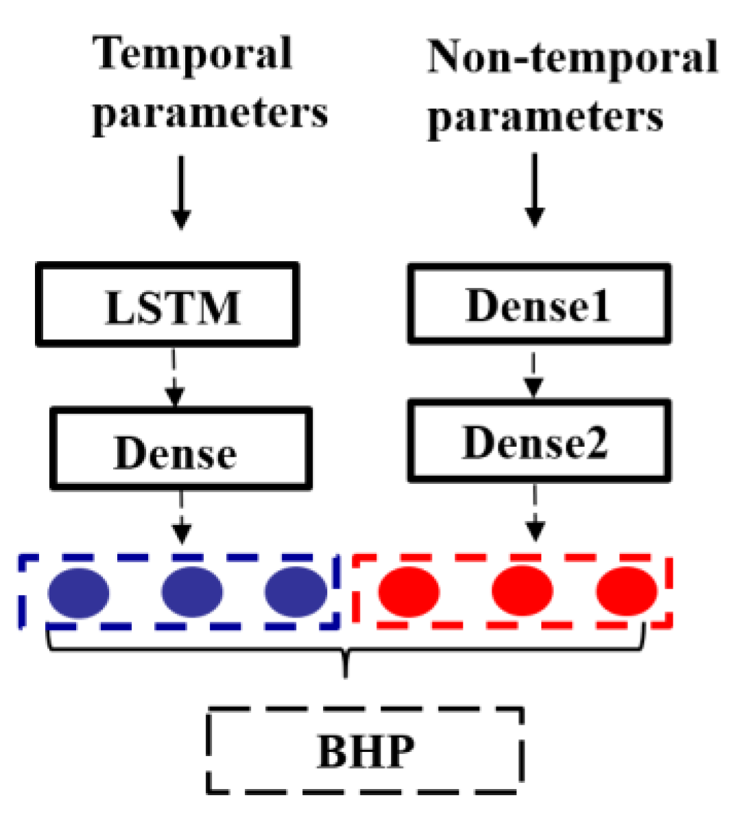
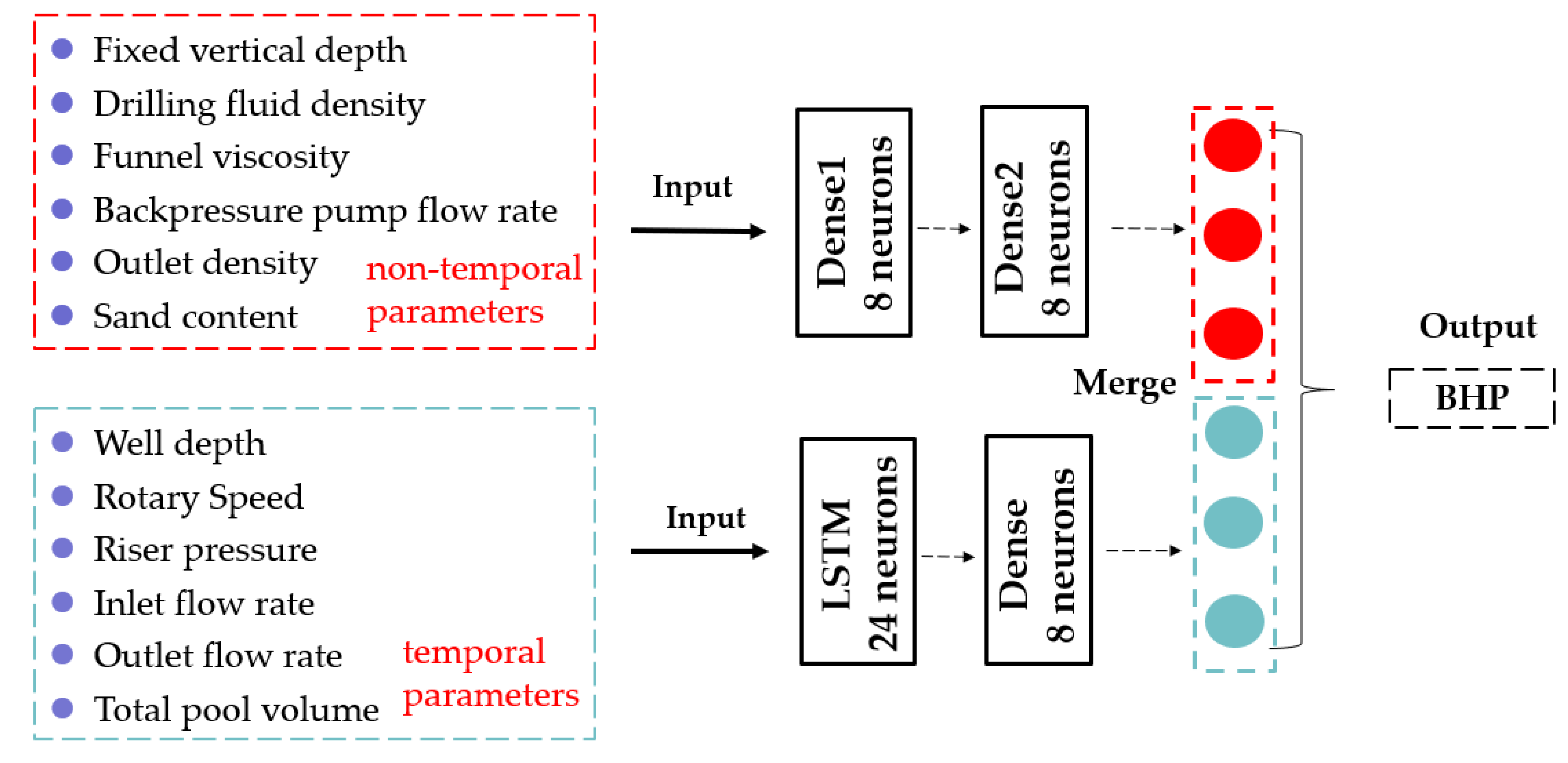
2.4. Parallel Network of BP and LSTM

From Section 2.1 and Section 2.2, the BP and LSTM networks each have their defects. The BP network has limited generalization ability for temporal multi-factor problems, and the LSTM network requires a certain length of sequence as training samples. Therefore, the prediction results of these two models alone do not have a high generalization ability. Considering the characteristics of the two models, this paper adopts the method of constructing a BP-LSTM hybrid model as shown in Figure 4 to input the sequential data into the LSTM network and the non-sequential data into the BP network, to give full play to the advantages of the two models and achieve a higher precision prediction of the models.

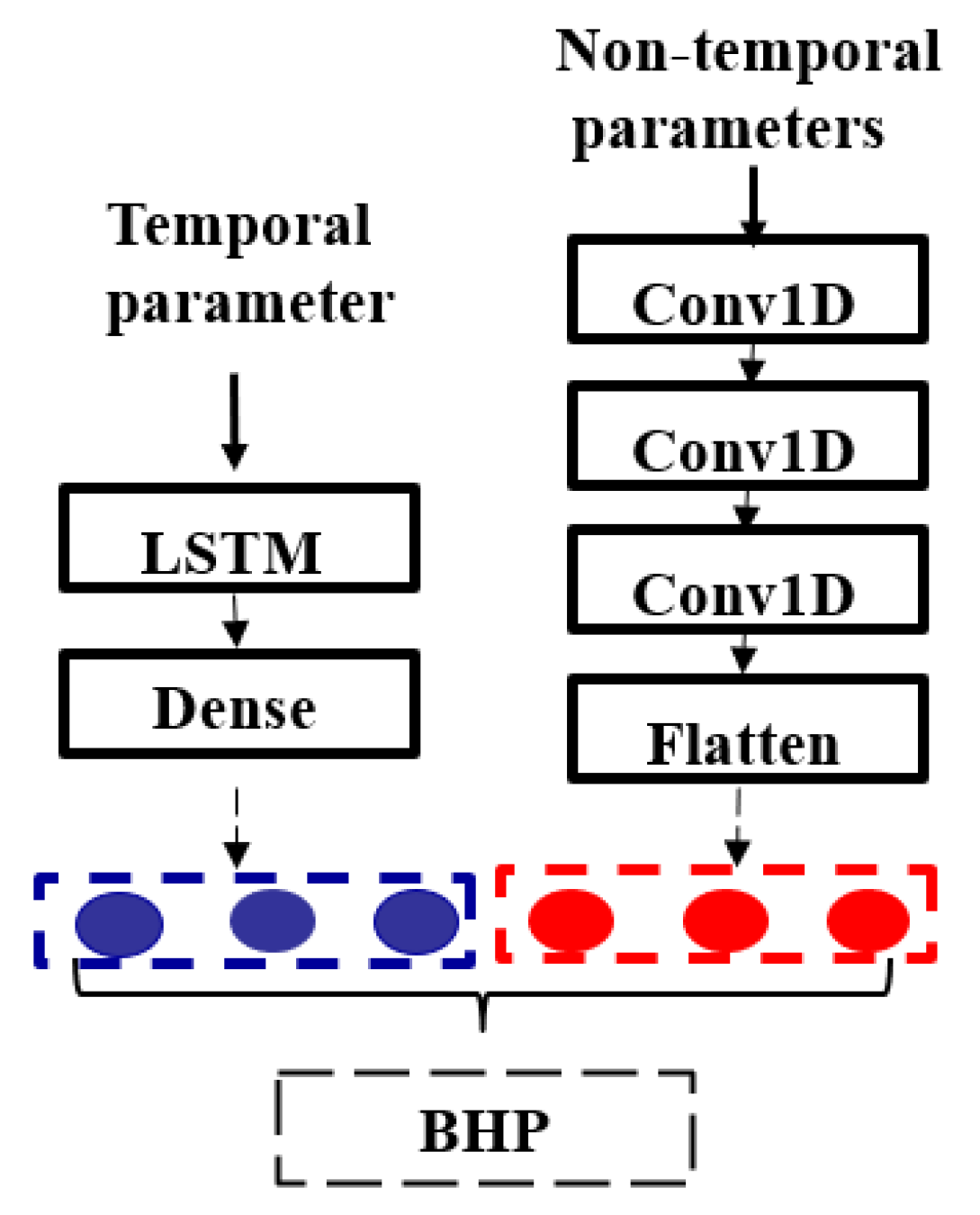
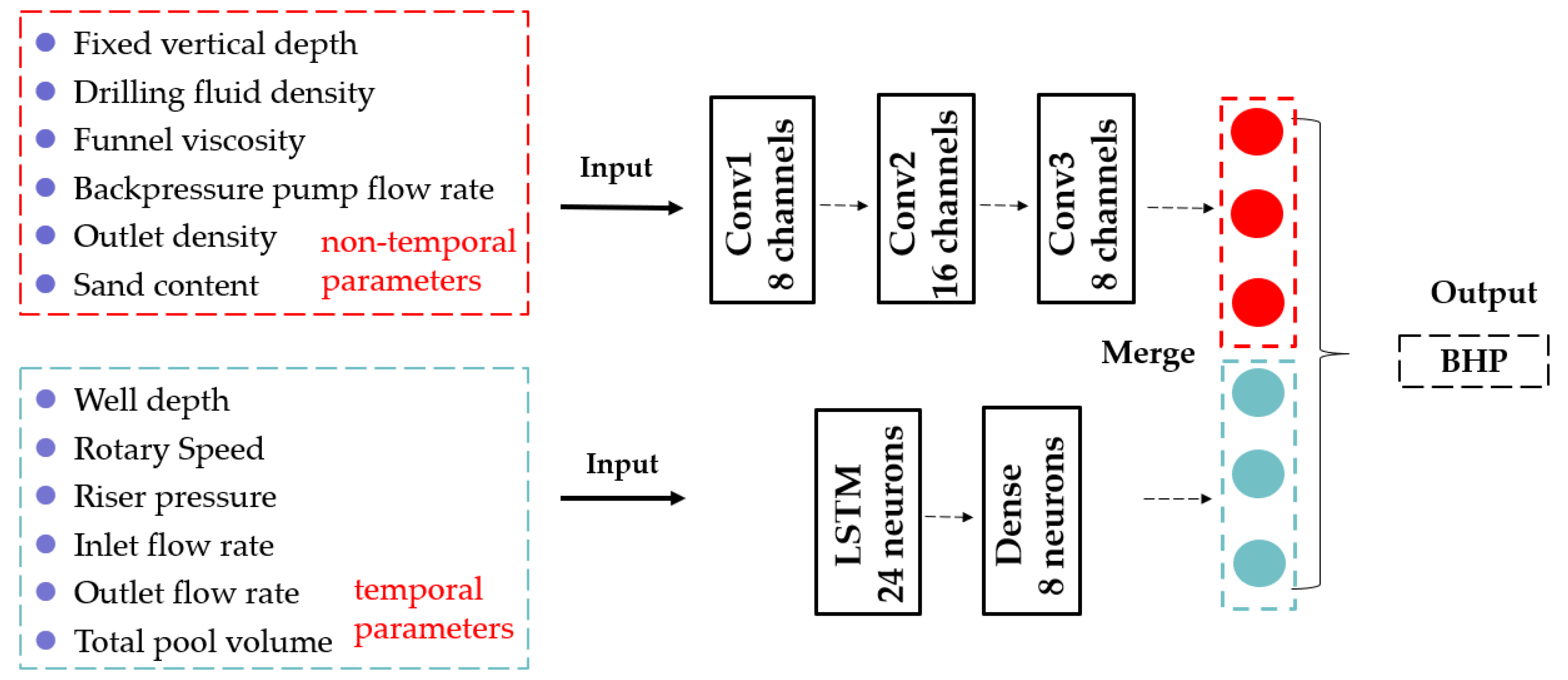
2.5. Parallel Network of 1DCNN and LSTM

The 1DCNN branch network mainly captures local correlation information through the convolution kernel, but the size of the convolution kernel limits the contextual relationship of a sequence captured by CNN, while the LSTM branch network can make up for this shortcoming by extracting sequential features. Therefore, a parallel network based on CNN and LSTM, shown in Figure 5, is proposed in this paper, which can significantly improve the effectiveness and accuracy of the BHP prediction model while extracting feature advantages from the network.

3. Dataset and Methodology

Based on the various network models proposed above, combined with the data preparation and model testing sessions, the complete BHP prediction process of this paper can be obtained as shown in Figure 6.

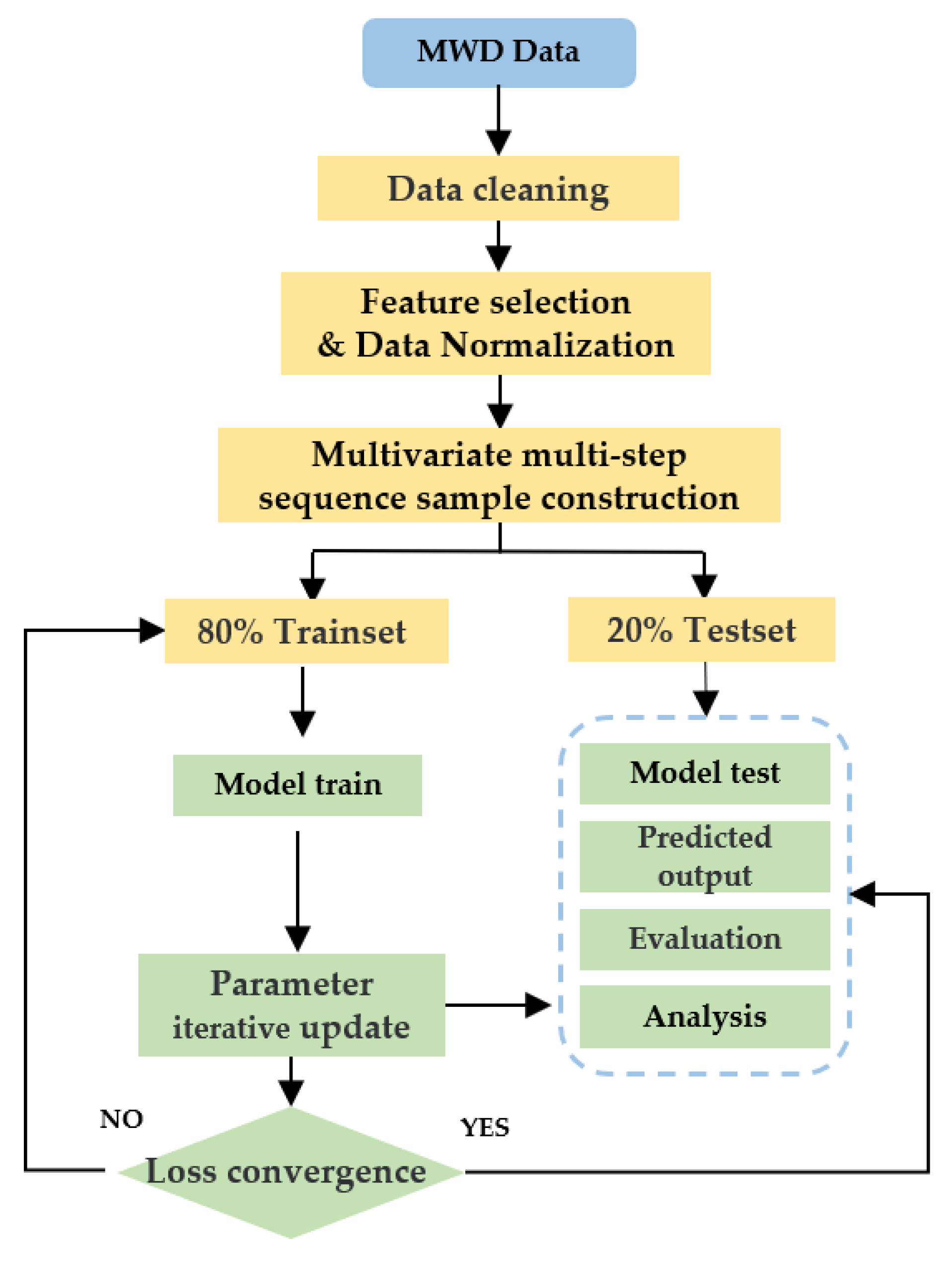
3.1. Data Pre-Processing

3.1.1. Data Description

In this paper, the basic data used to train and test the intelligent model are 130,000 sets of BHP measurements from surface monitoring, with a maximum measured depth of 6705 m and the maximum vertical depth of 4942 m. Firstly, the missing key drilling parameters were removed. At the same time, considering that the rheological parameters of drilling fluid have a similar single distribution, which plays a pivotal role in the performance of the model and will amplify the influence of subtle noise or lead to the high linearity of the model and reduce the stability of the model, this paper selectively supplements the performance parameters of drilling fluid, including funnel viscosity, s, sand content, %, and drilling fluid density, g/cm3. In addition, to check the validity of the data, empirical correlations and mechanistic models were used to estimate BHP, and the outliers were removed. Finally, 100,000 data points of pressure while drilling were used to train and test the model. The characteristics of BHP after cleaning are shown in Table 1.

3.1.2. Feature Selection and Data Normalization

In the process of drilling, BHP is related to many factors. Through correlation analysis, parameters that have a greater impact on BHP are selected, small or irrelevant variables are removed, input parameter dimensions are reduced, and the influence of noise is enlarged by the distance correlation coefficient due to the simultaneous introduction of two or more parameters with high similarity being avoided, as follows:
dCo r n 2 ( X , Y ) = { d C o v n 2 ( X , Y ) d C o v n 2 ( X ) d C o v n 2 ( Y ) d C o v n 2 ( X ) d C o v n 2 ( Y ) > 0   0 d C o v n 2 ( X ) d C o v n 2 ( Y ) = 0
where d C o r n 2 ( X , Y ) is the distance correlation coefficient of X and Y, d C o v n 2 ( X , Y ) is the distance covariance of X and Y, d C o v n 2 ( X ) is the standard deviation of the distance of X, and d C o v n 2 ( Y ) is the standard deviation of the distance of Y.
Parameters with a correlation greater than 0.7 were screened through calculation, and the following 12 input parameters were finally determined, as shown in Table 2, including 6 temporal parameters: well depth, rotary speed, riser pressure, inlet flow rate, outlet flow rate, total pool volume, and 6 non-timing parameters: drilling fluid density, funnel viscosity, fixed vertical depth, back-pressure pump flow rate, outlet density, and sand content.
The 100,000 filtered data points were divided into train sets and test sets. The train set of 80% (80,000 data points) was used to train the models, and the remaining dataset of 20% (20,000 data points)was used as a test set to test the prediction capabilities of the developed models.
Data normalization can speed up the gradient descent and the optimal solution for the characteristics between different dimensions, in a certain value of the comparability, and avoid excessive numerical problems in the process of training. Therefore, before model training, we need to normalize the processing of all input parameters and make all parameter mapping at the interval [0, 1], as shown in the following equation:
x ˜ = x x m i n x m a x x m i n
where x ˜ is the normalized value of x, x max and x min are the maximum and minimum values of the variable x.

3.1.3. Multivariate Multi-Step Sequence Sample Construction

Given that the MPD data collected in the field have a certain time series correlation, namely the data at the current well depth will have a certain influence on the lower well section, the prediction of BHP can be treated as a multi-variable sequential prediction problem, and the BHP at a certain depth can be predicted through the historical BHP.
Therefore, prior to training the model, it is necessary to prioritize the collection time of the original data set and convert it into supervised learning samples. Since there are multiple characteristic variables in managed pressure drilling data at each time point, and the predicted label has only one variable BHP, the other 12 characteristic variables can be deleted at the last time point when constructing sequence samples, so as to reduce data dimension and improve model operation efficiency. The fixed sequence of the unit length specified by the sliding window is used to calculate the indicators in the fixed sequence. The window size selected is 10, namely the sequence data of the first 10 s are used to predict the wellbore pressure of the next 10 s. The partial samples of the established multivariate sequence data are shown in Table 3.

3.2. Evaluation Indicators Selection

To evaluate the developed models and their predictive performances, in this paper, mean relative error (MRE), root mean square error (RMSE), and mean absolute error (MAE) are selected as the evaluation indicators of the network model. At the same time, this experiment adds additional model running time to the evaluation index to compare the model running efficiency.
M R E = 1 m i = 1 m | y i y p r e | y i
R M S E = 1 m i = 1 m ( y i y p r e ) 2
M A E = 1 m i = 1 m | y i y p r e |
where y i is the observed BHP values and y p r e is the calculated BHP values, which are predicted by the built models.

3.3. Model Establishment

3.3.1. Single Intelligence Models

In this study, we developed single intelligent prediction models with pytorch based on BP, LSTM, and 1DCNN. In order to make the models comparable and keep the model complexity consistent, all network parameters are set similarly. A sample input to the BP neural network is a one-dimensional vector, including 130 feature variables, and 13 features under each time step. A sample input of the LSTM network is a 10 × 13 matrix, which represents a time window of 10 and each time step contains 13 features. The 1DCNN network input sample is a 10 × 13 two-dimensional vector. The network contains three one-dimensional convolution layers (Conv1D) and one Flatten layer (Flatten), where the convolution kernel is 3, 3, and 2 in sequence, and the dropout probability is 0.2. The structure parameters of each network model are shown in Table 4.

3.3.2. Hybrid Parallel Intelligence Models

In this paper, based on the characteristics of the data, seven strong temporal and six weak temporal (non-temporal) feature parameters are filtered by analysis, and the strong temporal feature parameters are input into the LSTM network and the non-temporal feature parameters are input into the BP and CNN networks. Finally, the features are fully connected and fused to the output, so that the hybrid parallel network models of BP-LSTM and CNN-LSTM are established, as shown in Figure 7 and Figure 8. It should be noted that the hybrid network model is based on the fusion of the output features of a single intelligent model, so the network parameters of each branch remain the same as in Section 3.3.1.

4. Results and Discussion
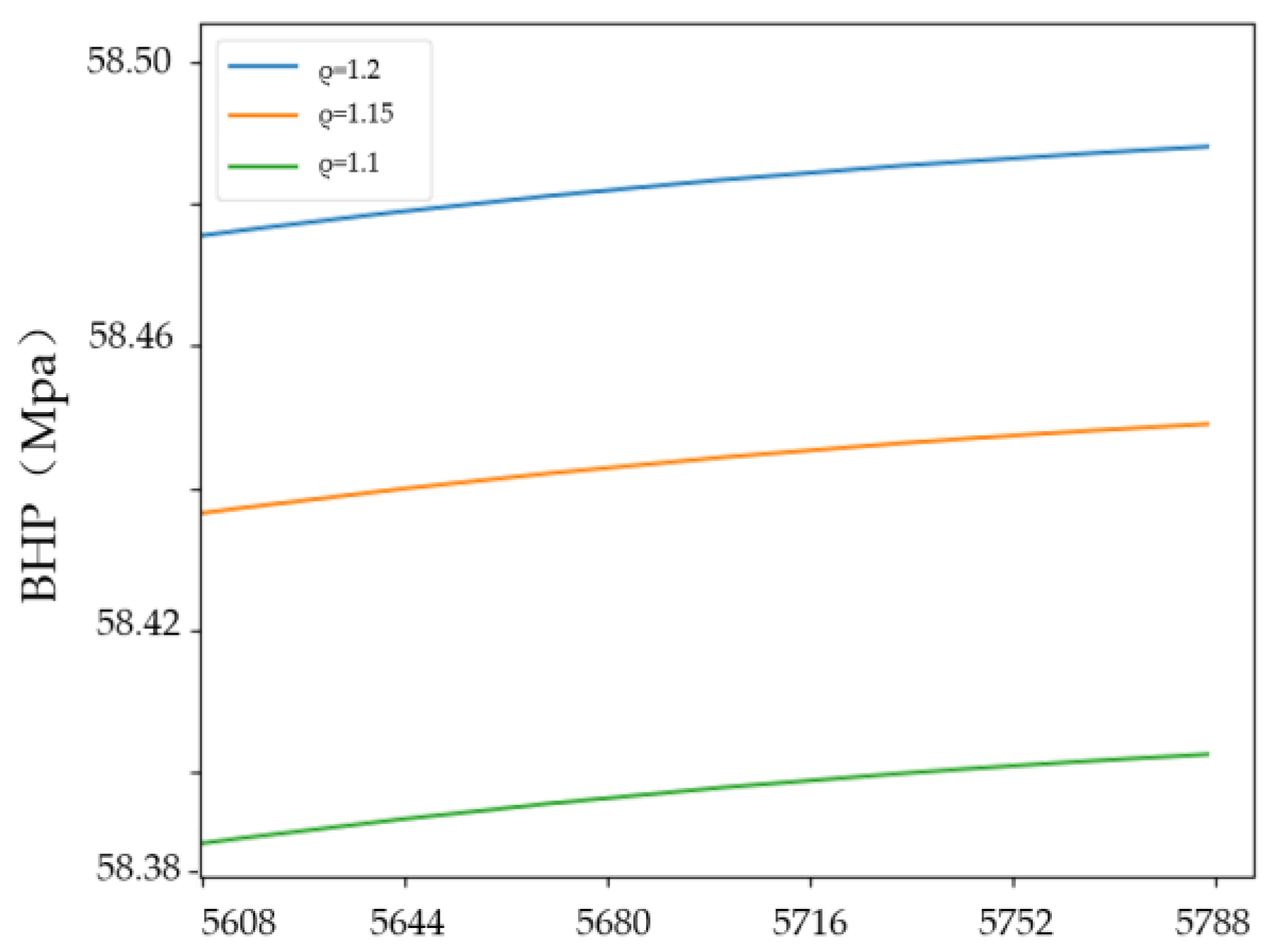
In this section, we compare and analyze the performance of the single bottomhole pressure intelligent prediction model and hybrid parallel intelligent prediction model on the test set, find the advantages of different models to capture features, and finally select and evaluate the best intelligent prediction model.
Observing the prediction results as shown in Table 5 reveals that the single intelligent models all exhibit similar volatility during the phase when the managed pressure drilling is maintained constant. The best relative performance is the LSTM model with a relative average error of 0.148%, while the relative average errors of BP and 1DCNN are 0.156% and 0.270%, respectively, and the stability of the models performs poorly. Specifically, the BP model captures the features of the time-series data more evenly and is good at dealing with the point-to-point mapping relationship without considering the contextual information of the time-series data. 1DCNN shows strong response fluctuations in the abrupt change phase of pressure-controlled drilling, and the model generates a larger feature map because of the relatively small number of channels, which leads to a large computation of the convolution process, so it takes up more memory and takes longer to run.
Further analysis shows that the prediction accuracy and stability of the two-hybrid parallel networks have significantly improved when compared with the single network. From Figure 9d,e, the excellent performance of the hybrid model in trend response and wave response is apparent. The CNN-LSTM parallel model has the best performance with an MAPE of 0.031% and the BP-LSTM has an MAPE of 0.040%, which are 78% and 72% lower than the optimal single intelligent model LSTM, respectively. In the CNN-LSTM parallel model, the feature parameters with weak temporal information are input into the CNN branch network and the feature parameters with strong temporal information are input into the LSTM branch network, which makes up for the shortcoming of the 1DCNN model with abnormal fluctuations at the pressure inflection point, making the prediction result more stable. In the BP-LSTM parallel model, the feature parameters with weak temporal information are input into the BP branch network and the feature parameters with strong temporal information are input into the LSTM branch network, which makes up for the volatile shortcomings of the single intelligent models of BP and LSTM in the pressure stabilization stage.
On the other hand, compared with the CNN-LSTM model, the BP-LSTM model still has local outliers at the pressure changes, and the fluctuation is more intense at the sudden change. Similar to 1DCNN, the CNN-LSTM parallel model has the longest running time, which is close to four to five times the running time of other models, which has also become one of the important factors to be considered in field practical applications.
Overall, these results indicate that the advantages of effectively fusing the extracted features of the model can further improve the accuracy and stability of the prediction model. The BP network extracts the feature information of the data with uniformity and is good at dealing with the point-to-point mapping relationship. The CNN network can accurately capture the subtle information between the data but finds it difficult to deal with the feature sequences with large fluctuations. The LSTM is good at considering the dependencies before and after the sequence. However, it finds it difficult to extract information with weak temporal information. Therefore, optimizing the hybrid model structure according to the actual feature of the field data is the key to improving the performance of the model.

5. Trend Analysis

Overall trend analysis can systematically assess the strength of the proposed model and make sure of how effectively the proposed model captures the physical phenomenon [16]. In this work, synthetic datasets were created, where in the dataset only one input parameter well depth was varied from its minimum to maximum values while all other parameters were kept constant at their average values. Figure 10 shows the effect of increasing well depth with three different drill fluid densities of 1.1, 1.15, and 1.2 g/cm3. It can be seen that in the horizontal direction, as the well depth is increasing, the BHP has a slowly increasing trend. Vertically, the bigger drilling fluid density makes a higher BHP. At the same time, observing the Y-axis, it is found that when the well depth reaches 5608 m, the drilling fluid density is changed from 1.1 to 1.2 g/cm3, and the BHP increases from 58.388 to 58.474 MPa, which proves the robustness of the model. This trend can also be further demonstrated by the momentum equation. To sum up, the trend analysis shows that the CNN-LSTM hybrid model can capture the correct physics behind the data and has a certain stability.

6. Conclusions

The contribution of this paper is to predict the BHP accurately and optimize the processing of temporal data in managed pressure drilling.
The BP model captures time-series data with uniformity, the LSTM model can effectively extract the contextual information of the time-series data, and the CNN model pays more attention to capturing the subtle changes of the data. The hybrid optimization model that combines the advantages of a single intelligent model can significantly reduce the predicted outliers, improve the accuracy and stability, and reduce the average relative error by about 70%.
The CNN-LSTM model has a strong ability to extract the time-series characteristics of the pressure-while-drilling data and can capture the subtle changes, with an average relative error of 0.031%. However, due to the influence of the size of the convolution kernel, the feature map formed after convolution is large, which reduces the efficiency of model solving, and the running time is about 4.5 times higher than that of the BP-LSTM parallel model. Through trend analysis, the effectiveness and robustness of the CNN-LSTM model is demonstrated.
This research can further predict BHP accurately by using a hybrid model method and create a more robust model to deal with complex situations in the field. In the future, we hope to intelligently select the appropriate model according to the time-series characteristics of the data and explore interpretable methods to correctly capture the physical meaning behind the MWD data.

Author Contributions

Conceptualization, Z.Z. and X.S.; methodology, Z.Z.; software, R.Z.; validation, Z.Z., X.S. and R.Z.; formal analysis, Z.Z.; investigation, Z.Z.; resources, X.S.; data curation, R.Z.; writing—original draft preparation, R.Z.; writing—review and editing, Z.Z., L.H., X.H., D.L. and D.Y.; visualization, R.Z. and F.Q.; supervision, Z.Z.; project administration, Z.Z.; funding acquisition, X.S and G.L. All authors have read and agreed to the published version of the manuscript.

Funding

This research was funded by China National Petroleum Corporation Limited–China University of Petroleum (Beijing) strategic cooperation science and Technology special project, grant number ZLZX2020-03, National Science Foundation for Distinguished Young Scholars, grant number 52125401, Science Foundation project of China University of Petroleum (Beijing), grant number 2462022SZBH002 and National Key RESEARCH and Development Program of China, “Key Scientific Issues of Transformative Technologies”, grant number 2019YFA0708300.

Institutional Review Board Statement

Not applicable.

Informed Consent Statement

Not applicable.

Data Availability Statement

The data are not publicly available due to involve the information of Chinese oil fields and need to be kept confidential.

Acknowledgments

The author would like to thank the academic salon of the High-Pressure Water Jet Drilling and Completion Laboratory of China University of Petroleum (Beijing), and Wang Tianyu for giving constructive suggestions and ideas, which helped improve the quality of the paper.

Conflicts of Interest

The authors declare no conflict of interest.

References

  1. Sami, N.A.; Ibrahim, D.S. Forecasting multiphase flowing bottom-hole pressure of vertical oil wells using three machine learning techniques. Pet. Res. 2021, 6, 417–422. [Google Scholar] [CrossRef]
  2. Aziz, K.; Govier, G.W. Pressure Drop In Wells Producing Oil And Gas. J. Can. Pet. Technol. 1972, 11, 30940. [Google Scholar] [CrossRef]
  3. Chokshi, R.N.; Schmidt, Z.; Doty, D.R. Experimental Study and the Development of a Mechanistic Model for Two-Phase Flow Through Vertical Tubing. In Proceedings of the SPE Western Regional Meeting, Anchorage, AK, USA, 22–24 May 1996. [Google Scholar]
  4. Ansari, A.M.; Sylvester, N.D.; Sarica, C.; Shoham, O.; Brill, J.P. A Comprehensive Mechanistic Model for Upward Two-Phase Flow in Wellbores. SPE Prod. Facil. 1994, 9, 143–151. [Google Scholar] [CrossRef] [Green Version]
  5. Duns, H., Jr.; Ros, N.C.J. Vertical flow of gas and liquid mixtures in wells. In Proceedings of the 6th World Petroleum Congress, Frankfurt am Main, Germany, 19–26 June 1963. [Google Scholar]
  6. Gomez, L.E.; Shoham, O.; Schmidt, Z.; Chokshi, R.N.; Northug, T. Unified Mechanistic Model for Steady-State Two-Phase Flow: Horizontal to Vertical Upward Flow. SPE J. 2000, 5, 339–350. [Google Scholar] [CrossRef]
  7. Hagedorn, A.R.; Brown, K.E. Experimental Study of Pressure Gradients Occurring During Continuous Two-Phase Flow in Small-Diameter Vertical Conduits. J. Pet. Technol. 1965, 17, 475–484. [Google Scholar] [CrossRef]
  8. Orkiszewski, J. Predicting Two-Phase Pressure Drops in Vertical Pipe. J. Pet. Technol. 1967, 19, 829–838. [Google Scholar] [CrossRef]
  9. Ternyik, J., IV; Bilgesu, H.I.; Mohaghegh, S.; Rose, D.M. Virtual Measurement in Pipes: Part 1-Flowing Bottom Hole Pressure Under Multi-Phase Flow and Inclined Wellbore Conditions. In Proceedings of the SPE Eastern Regional Meeting, Morgantown, West Virginia, 17–21 September 1995. [Google Scholar]
  10. Mohammadpoor, M.; Shahbazi, K.; Torabi, F.; Qazvini, A. A New Methodology for Prediction of Bottomhole Flowing Pressure in Vertical Multiphase Flow in Iranian Oil Fields Using Artificial Neural Networks (ANNs). In Proceedings of the SPE Latin American and Caribbean Petroleum Engineering Conference, Lima, Peru, 1–3 December 2010. [Google Scholar]
  11. Jahanandish, I.; Salimifard, B.; Jalalifar, H. Predicting bottomhole pressure in vertical multiphase flowing wells using artificial neural networks. J. Pet. Sci. Eng. 2011, 75, 336–342. [Google Scholar] [CrossRef]
  12. Chen, W.; Di, Q.; Ye, F.; Zhang, J.; Wang, W. Flowing bottomhole pressure prediction for gas wells based on support vector machine and random samples selection. Int. J. Hydrogen Energy 2017, 42, 18333–18342. [Google Scholar] [CrossRef]
  13. Spesivtsev, P.; Sinkov, K.; Sofronov, I.; Zimina, A.; Umnov, A.; Yarullin, R.; Vetrov, D. Predictive model for bottomhole pressure based on machine learning. J. Pet. Sci. Eng. 2018, 166, 825–841. [Google Scholar] [CrossRef]
  14. Mask, G.; Wu, X.; Ling, K. An improved model for gas-liquid flow pattern prediction based on machine learning. J. Pet. Sci. Eng. 2019, 183, 106370. [Google Scholar] [CrossRef]
  15. Okoro, E.E.; Obomanu, T.; Sanni, S.E.; Olatunji, D.I.; Igbinedion, P. Application of artificial intelligence in predicting the dynamics of bottom hole pressure for under-balanced drilling: Extra tree compared with feed forward neural network model. Petroleum 2021, 8, 227–236. [Google Scholar] [CrossRef]
  16. Tariq, Z.; Mahmoud, M.; Abdulraheem, A. Real-time prognosis of flowing bottom-hole pressure in a vertical well for a multiphase flow using computational intelligence techniques. J. Pet. Explor. Prod. Technol. 2019, 10, 1411–1428. [Google Scholar] [CrossRef] [Green Version]
  17. Nait Amar, M.; Zeraibi, N.; Redouane, K. Bottom hole pressure estimation using hybridization neural networks and grey wolves optimization. Petroleum 2018, 4, 419–429. [Google Scholar] [CrossRef]
  18. Irani, R.; Nasimi, R. Application of artificial bee colony-based neural network in bottom hole pressure prediction in underbalanced drilling. J. Pet. Sci. Eng. 2011, 78, 6–12. [Google Scholar] [CrossRef]
  19. Ashena, R.; Moghadasi, J. Bottom hole pressure estimation using evolved neural networks by real coded ant colony optimization and genetic algorithm. J. Pet. Sci. Eng. 2011, 77, 375–385. [Google Scholar] [CrossRef]
  20. Barati-Harooni, A.; Najafi-Marghmaleki, A.; Tatar, A.; Arabloo, M.; Phung, L.T.K.; Lee, M.; Bahadori, A. Prediction of frictional pressure loss for multiphase flow in inclined annuli during Underbalanced Drilling operations. Nat. Gas Ind. B 2016, 3, 275–282. [Google Scholar] [CrossRef]
  21. Liang, H.; Wei, Q.; Lu, D.; Li, Z. Application of GA-BP neural network algorithm in killing well control system. Neural Comput. Appl. 2021, 33, 949–960. [Google Scholar] [CrossRef]
  22. Fruhwirth, R.K.; Thonhauser, G.; Mathis, W. Hybrid Simulation Using Neural Networks To Predict Drilling Hydraulics in Real Time. In Proceedings of the SPE Annual Technical Conference and Exhibition, San Antonio, TX, USA, 24–27 September 2006. [Google Scholar]
  23. Elzenary, M.; Elkatatny, S.; Abdelgawad, K.Z.; Abdulraheem, A.; Mahmoud, M.; Al-Shehri, D. New Technology to Evaluate Equivalent Circulating Density While Drilling Using Artificial Intelligence. In Proceedings of the SPE Kingdom of Saudi Arabia Annual Technical Symposium and Exhibition, Dammam, Saudi Arabia, 23–26 April 2018. [Google Scholar]
  24. Al Shehri, F.H.; Gryzlov, A.; Al Tayyar, T.; Arsalan, M. Utilizing Machine Learning Methods to Estimate Flowing Bottom-Hole Pressure in Unconventional Gas Condensate Tight Sand Fractured Wells in Saudi Arabia. In Proceedings of the SPE Russian Petroleum Technology Conference, Virtual, 26–29 October 2020. [Google Scholar]
  25. Li, X.; Miskimins, J.L.; Hoffman, B.T. A Combined Bottom-hole Pressure Calculation Procedure Using Multiphase Correlations and Artificial Neural Network Models. In Proceedings of the SPE Annual Technical Conference and Exhibition, Amsterdam, The Netherlands, 27–29 October 2014. [Google Scholar]
  26. Gola, G.; Nybø, R.; Sui, D.; Roverso, D. Improving Management and Control of Drilling Operations with Artificial Intelligence. In Proceedings of the SPE Intelligent Energy International, Utrecht, The Netherlands, 27–29 March 2012. [Google Scholar]
  27. Wiśniowski, R.; Skrzypaszek, K.; Małachowski, T. Selection of a Suitable Rheological Model for Drilling Fluid Using Applied Numerical Methods. Energies 2020, 13, 3192. [Google Scholar] [CrossRef]
  28. Sheu, B.J.; Choi, J. Back-Propagation Neural Networks. In Neural Information Processing and VLSI; Springer: Boston, MA, USA, 1995; pp. 277–296. [Google Scholar] [CrossRef]
  29. Gers, F.A.; Schmidhuber, J.; Cummins, F. Learning to Forget: Continual Prediction with LSTM. Neural Comput. 2000, 12, 2451–2471. [Google Scholar] [CrossRef] [PubMed]
Figure 1. Schematic diagram of BP neural network with one hidden layer where xn is the current input; i is the input layer; h is the hidden layer; wih and wjk are the weight matrix of the hidden layer; o is the output layer and yn is the current output.
Applsci 12 06728 g001
Figure 2. Self-circulating structure in LSTM where xt is the current input; ht−1 is the output at the previous moment; ht is the current output; Ct−1 is the previous cell state; Ct is the current cell state; ft is the forget gate neuron in LSTM The output of the cell; it is the output of the input gate neuron in LSTM; C ˜ t is the new candidate values for cell status; Ot is the output of the output gate neuron in LSTM; σ is the sigmoid activation function and tanh is the tanh activation function.
Applsci 12 06728 g002
Figure 3. The structure of 1DCNN.
Applsci 12 06728 g003
Figure 4. BP-LSTM parallel network structure.
Applsci 12 06728 g004
Figure 5. CNN-LSTM parallel network structure.
Applsci 12 06728 g005
Figure 6. Process of BHP output forecasting.
Applsci 12 06728 g006
Figure 7. BP-LSTM parallel network internal detailed structure.
Applsci 12 06728 g007
Figure 8. CNN-LSTM parallel network internal detailed structure.
Applsci 12 06728 g008
Figure 9. Comparison and evaluation results of real and predicted BHP. (a) The prediction results of BP network; (b) The prediction results of LSTM network; (c) The prediction results of 1DCNN; (d) The prediction results of BP-LSTM parallel network; (e) The prediction results of CNN-LSTM parallel network; (f) Performance evaluation results of various models.
Applsci 12 06728 g009
Figure 10. Effect of changing well depth on BHP with different drilling fluid density.
Applsci 12 06728 g010
Table 1. Data description of BHP.
Evaluation StandardValueEvaluation StandardValue
Count60,00025% (Mpa)58.26
Mean (Mpa)58.6150% (Mpa)58.70
Std (Mpa)0.4075% (Mpa)58.70
Min (Mpa)57.37Max (Mpa)59.58
Table 2. Input and output parameters of the model.
Input ParametersOutput Parameter
Temporal parametersWell depth, Rotary speed, Riser pressure, Inlet flow rate, Outlet flow rate, Total pool volumeBHP
Non-temporal parametersFixed vertical depth, Drilling fluid density,
Funnel viscosity, Back-pressure pump flow rate, Outlet density, Sand content
Table 3. Sample of multivariable sequence data.
Var6(t−1)var7(t−1)var8(t−1)var9(t−1)var13(t−1)
0.000380.9572120.8496030.0097180.799
0.000420.9572290.8798540.0183510.799
0.000460.9572420.8675510.0167180.799
0.000500.9572630.8554360.0268370.799
0.000580.957280.8815100.0200170.799
Table 4. The structure parameters of BP, LSTM and 1DCNN network model.
ParameterBPLSTM1DCNN
Model parameter324939533769
Time steps/1010
Batch size600600600
Learning rate0.0010.0010.001
OptimizerAdamAdamAdam
Activation functionReluReluRelu
Hidden layer neurons/
Channels
Dense1: 8; Dense2: 8LSTM: 24; Dense: 8Conv1: 8; Conv2: 16; Conv3: 8
Table 5. Experimental evaluation results.
Evaluation IndicatorBPLSTM1DCNNBP-LSTMCNN-LSTM
Run time (s)30.04239.034160.71145.089200.640
MAPE (%)0.1560.1480.2700.0400.031
MAE0.0920.0870.1580.0230.018
RMSE0.1170.1060.2550.0490.047
Publisher’s Note: MDPI stays neutral with regard to jurisdictional claims in published maps and institutional affiliations.

